Interactive Learning of Pattern Rankings
Vladimir Dzyuba, Matthijs van Leeuwen, Siegfried Nijssen⇤, Luc De Raedt
Department of Computer Science, KU Leuven Celestijnenlaan 200A – bus 2402, Leuven, 3000, Belgium
{vladimir.dzyuba, matthijs.vanleeuwen, siegfried.nijssen, luc.deraedt}@cs.kuleuven.be
Received (Day Month Year) Revised (Day Month Year) Accepted (Day Month Year)
Pattern mining provides useful tools for exploratory data analysis. Numerous efficient algorithms exist that are able to discover various types of patterns in large datasets. Unfortunately, the problem of identifying patterns that are genuinely interesting to a particular user remains challenging. Current approaches generally require considerable data mining expertise or e↵ort from the data analyst, and hence cannot be used by typical domain experts.
To address this, we introduce a generic framework for interactive learning of user-specific pattern ranking functions. The user is only asked to rank small sets of patterns, while a ranking function is inferred from this feedback by preference learning techniques. Moreover, we propose a number of active learning heuristics to minimize the e↵ort re-quired from the user, while ensuring that accurate rankings are obtained. We show how the learned ranking functions can be used to mine new, more interesting patterns.
We demonstrate two concrete instances of our framework for two di↵erent pattern mining tasks, frequent itemset mining and subgroup discovery. We empirically evaluate the capacity of the algorithm to learn pattern rankings by emulating users. Experiments demonstrate that the system is able to learn accurate rankings, and that the active learning heuristics help reduce the required user e↵ort. Furthermore, using the learned ranking functions as search heuristics allows discovering patterns of higher quality than those in the initial set. This shows that machine learning techniques in general, and active preference learning in particular, are promising building blocks for interactive data mining systems.
Keywords: Interactive data mining; preference learning; active learning; pattern mining. 1. Introduction
Large amounts of data are available nowadays. Making sense of this data and putting it to good use is a major challenge in many domains, ranging from academic research to practical commercial applications. However, the large sizes of datasets make manual processing and analysis virtually impossible. Automated tools that alleviate these issues are the subject of research in data mining and knowledge discovery. ⇤Also affiliated with Leiden Institute for Advanced Computer Science, Leiden University, The
Netherlands.
Pattern mining is an important concept in data mining that aims at discovering patterns from data. Informally, a pattern is an expression in a certain language that concisely describes some local structure in the dataset. Many variations of pattern mining have been proposed in the literature, and many algorithms for efficiently mining patterns from large datasets exist. For example, subgroup discovery29
con-cerns patterns in labeled data, i.e., descriptions of regions in the data characterized by an unusual distribution of the property of interest. In the context of a bank pro-viding loans, the fact that 16% of loans withpurpose=used carare not repaid may be an interesting subgroup pattern, in particular given the fact that the baseline of unpaid loans is only 5%.
Unfortunately, the adoption of pattern mining techniques by domain experts is still limited in practice. One common problem is the so-called pattern explosion: large numbers of patterns are often discovered, of which many are very similar and hence redundant. Consequently, a domain expert has to invest substantial e↵ort to identify those patterns that are relevant to her specific interests and goals. Manual filtering of the results or tuning algorithm parameters are hardly e↵ective solutions and certainly hard for domain experts. Top-k mining and particularly pattern set mining28,33are techniques that specifically address the redundancy problem; in both
cases, the number of discovered patterns is limited.
Still, these existing approaches have a number of inherent problems, which cor-respond with the interestingness measure used.Objective interestingness measures, on one hand, only concern the structure of the data and do not take into account knowledge and goals of a user. As a result, re-discovery of common knowledge is a typical problem, even when redundancy is successfully avoided. Subjective inter-estingness measures, on the other hand, account for the user-specific context via a model of the dataset or of the entire domain. But then, an expert has to be familiar with the particular model type being used, e.g., Bayesian networks. This shifts the problem of the user from filtering results to specifying the right model, which is yet another non-trivial task and requires expertise beyond the problem domain.
1.1. Learning task- and user-specific interestingness
In practice, pattern interestingness heavily depends on the specific task and user characteristics, such as analysis goals and background knowledge. Developing prin-cipled methods to account for such information is key to broadening the adoption of pattern mining as a generic technique for knowledge discovery. Because of this strong dependency, we argue that direct involvement of the user in the mining pro-cess is essential. We propose to frame the problem asinteractive learning and mining loop that consists of three major steps:
(1) Mining patterns.
In this step, a mining algorithm is used to find patterns that are to be pre-sented to the user. It is crucial that the mining algorithm allows some form of subjective input. In general, this input is initially empty, and mining is
essen-tially objective. However, in later iterations, an increasingly precise model of user interests becomes available, which allows for discovering subjectively more interesting patterns.
(2) Interacting with the user.
The patterns are presented to the user, who can freely explore and inspect them. Meanwhile, feedback is elicited from the user, either implicitly or explicitly. The feedback to the learning system should be simple in order for the system to be accessible to non-data mining experts, yet at the same time should convey enough information about the user’s interests.
(3) Learning user-specific pattern interestingness.
The elicited feedback is used to build and improve the model of the user inter-ests, i.e., to identify what makes patterns interesting to the user. Most impor-tantly, the learned model is used in the next mining iteration, so that the e↵ort required to achieve the analysis goals is minimized.
This generic loop can be paraphrased by the adage “Mine, interact, learn, re-peat”. Naturally, each step of the loop entails a number of important design choices. Questions that need to be answered include how to organize user interaction, how to model subjective interestingness, how to learn such models from user feedback, and how to incorporate subjective interestingness into pattern mining.
1.2. Approach and contributions
In this paper, we propose a concrete instance of the interactive learning and min-ing loop that is based on the notion of pattern rankings. For this, we build upon our recent work10, of which the current article is a substantially extended version. We will now outline our approach and contributions in more detail, and explicitly mention the novel contributions of this extended paper.
In our approach, which was initially introduced in our earlier work10, we model user-specific interestingness as a total order over patterns. That is, for any two patterns from a given pattern language, one of the two is deemed more interesting than the other. This results in a ranking over patterns, such that the most interesting patterns are ranked highest. It is such a pattern ranking that we would like to learn through interaction with the user.
To achieve this, we make the following assumptions about the user:
(1) A user has an implicit preference between any pair of patterns, which does not change during a particular analysis session;
(2) The costs of eliciting the complete preference relation, or pattern ranking, i.e., expressing it in any analytical or other form, are prohibitively high;
(3) For any single pair of patterns, however, the user can accurately identify which of the two she prefers, i.e., which pattern she considers more interesting. Our first main contribution is a generic algorithm for the interactive learning of pattern rankings, which are represented by means of ranking functions. That is, we
employ a preference learning algorithm to infer a ranking function that can score any pattern in the pattern language considered. The absolute scores provided by this function are unimportant, but the relative scores define the ranking over the com-plete pattern space. Ranking functions are functions over a feature representation of the patterns, so that feature relevance can be learned from user feedback.
Feedback elicited from the user amounts to rankings of small sets of patterns, to which we will refer as queries in this paper. Executing a query implies that the system selects a few patterns, presents these to the user, and asks the user to rank them. By generalizing from the pattern rankings provided by the user to such queries, a subjective pattern interestingness measure is learned. We propose and evaluate a number of active query selection methods, which aim to minimize the feedback –and thus e↵ort– required from the user, while ensuring that accurate ranking functions are learned.
When mining the initial patterns, no knowledge about the user is known. There-fore, the user can select an objective interestingness measure based on her prior be-liefs. This interestingness measure determines the initial source ranking; the closer this ranking is to the subjective target ranking that is to be learned, the easier the learning task becomes. When a pool of patterns has been mined, queries can be selected and presented to the user. The ranking function is then updated based on feedback provided by the user, and then the learned ranking function is used to mine novel, hopefully more interesting patterns.
The second main contribution isthe application of the proposed approach in the context of two well-known pattern mining settings, i.e., frequent itemset mining and subgroup discovery. The former concerns the discovery of items that frequently co-occur in unlabeled, transactional data, whereas the latter concerns the discovery of subsets of labeled data for which the labels deviate from the overall distribution. Our previous work only considered subgroup discovery, hence the application to frequent itemset mining is a novel contribution of this paper.
The remainder of this paper is organized as follows. First, Sections 2 and 3 describe related work and preliminaries respectively. Then, Section 4 describes a toy example to illustrate how our framework interactively learns pattern rankings. Section 5 introduces our framework for learning pattern rankings, consisting of both a problem definition and detailed algorithm description, after which Section 6 discusses how to use the learned ranking functions for mining new patterns.
Section 5 presents the extensive (and extended) experimental evaluation, for both frequent itemset mining and subgroup discovery. In order to perform a prin-cipled and objective evaluation of our methods, we emulate user preferences over patterns using several existing interestingness measures. The results show that the algorithm is able to learn accurate pattern rankings, and that query selection heuris-tics help reduce the amount of input required for learning. Moreover, the learned ranking functions generalize well and allow discovering novel high-quality patterns when used for mining. After that, we round up with a discussion and conclusions in Sections 8 and 9.
2. Related work
In this section we describe work that is most closely related to ours, on the topic of subjective interestingness and interactive pattern mining on one hand, and on the topic of preference learning on the other hand.
Subjective interestingness and interactive pattern mining The importance of taking user knowledge and goals into account in order to discover genuinely in-teresting patterns was first emphasized by Tuzhilin25 in 1995. Nevertheless, most works concerning user-specific pattern interestingness measures and interactive pat-tern mining are fairly recent26. These approaches can be divided into three groups:
1) specifying a model of user interests in advance; 2) using user feedback to directly influence the search procedure; and 3) learning an explicit model of user interests.
Modeling user interests The approach by Jaroszewicz et al.13 allows a user
to specify a Bayesian network that represents beliefs about the data-generating process. The algorithm then finds surprising attribute sets, i.e., attribute sets for which the discrepancy between the expected and observed frequencies is larger than a certain threshold. The search is based on efficiently computing (or approximating) a large number of marginal distributions. A user can then manually update the Bayesian network, i.e., her beliefs, based on the inspected patterns, and subsequently repeat the mining process. One disadvantage of this approach is that it does not avoid the pattern explosion, at least not without tuning a threshold.
De Bie8 has developed a general framework for exploratory data analysis that
uses information theory to formalize subjective interestingness as surprisingness with respect to certain prior beliefs. Di↵erent types of prior beliefs can be used, for example, expected frequencies of individual items. Given these prior beliefs, a Max-imum Entropy distribution is fit to represent the expected data. This distribution is then used to quantify how informative the pattern is, given the beliefs. The frame-work lends itself well to iterative data mining: starting from a model based solely on prior beliefs, one can look for the subjectively most interesting pattern, which can then be added to the model. Hence, the next discovered pattern will automatically be substantially di↵erent from the previous one; this helps avoiding redundancy. A disadvantage of this framework is that it currently only allows for scoring pre-mined pattern collections, but not for directly mining high-scoring patterns.
Interactive search Bhuiyan et al.3 proposed a technique that is based on Markov Chain Monte Carlo sampling of frequent itemsets. User interests are mod-eled via a scoring function that is a product of weights of individual items; the probability of sampling an itemset is proportional to its score. In each iteration, a user inspects a small set of sampled itemsets and provides feedback by liking
or disliking them. This feedback is then used to update the weights: the weights of items comprising liked (resp. disliked) itemsets are increased (resp. decreased).
As a result, itemsets that are more similar to liked ones become more likely to be sampled and presented to the user. Sampling itemsets allows avoiding pattern ex-plosion, while still ensuring obtaining a sample of the complete set of patterns that is representative according to the (current) sampling distribution.
Dzyuba and Van Leeuwen9developed a similar approach for interactive subgroup
discovery. They augment a beam search-based subgroup discovery algorithmDSSD
with interactive beam selection: at each level, a user is allowed to inspect subgroups in the current beam andlikeordislikethem. This feedback is used to prune the beam and to re-weigh an objective subgroup quality measure, which essentially becomes subjective. The goal is to steer the search towards patterns that are more similar to the liked ones. Even though the algorithm uses a naive scheme to accomplish this, which does not always have predictable outcomes, it has been shown to improve the results from the subjective standpoint of a domain expert.
Learning models of user interests Preference learning has been previously used to identify interesting patterns in an interactive manner. Xin et al.30 investigated
learning a user-specific ranking of frequent patterns (primarily itemsets and se-quences). A clustering-based method similar to information retrieval approaches is used to select patterns for feedback. However, they only consider a specific learning target based on the discrepancy between the expected and observed supports of a pattern, and they do not use the learned functions to search for novel patterns.
Rueping22demonstrated the feasibility of learning subgroup rankings and
apply-ing learned rankapply-ing functions to discover high-quality subgroups. However, Ruepapply-ing does not discuss active learning aspects and uses a custom variant of the learner and data modifications that are specific to subgroup discovery. Therefore, it cannot be straightforwardly generalized to other pattern mining tasks, as we do in this paper. TheOne Click Mining system 4 is a generic system for interactive data mining that is not restricted to a single pattern type. That is, contrary to our system, it considers multiple types of patterns at once. Essentially, it learns two types of preferences simultaneously. On one hand, it uses a multi-armed bandit strategy to learn which mining algorithms discover the patterns that are most positively evaluated by a user. For example, that the user prefers subgroups with a particular target to itemsets. These preferences are used to allocate computation time to the di↵erent algorithms. On the other hand, co-active learning is used to learn a pattern ranking function fromimplicit user feedback, i.e., the actions performed by the user in the graphical user interface. Conceptually, this system is very similar to the one proposed in this paper, using similar techniques. Still, there are a number of key di↵erences. One such di↵erence is that One Click Mining only mines objectively interesting patterns, i.e., the learned ranking function is not used in the mining phase. Another di↵erence is that although we show that our framework is generic enough to deal with di↵erent types of patterns, we choose to focus on one mining task at a time, mainly for reasons of transparency and ease of use for the user.
Recently, Negrevergne et al.19 proposed dominance programming, a declarative
language that allows one to explicitly specify pairwise preferences between patterns, which are then used to find a complete set of non-dominated patterns. Only mod-eling objective preferences has been studied so far; learning models from example preferences is an open research question.
Preference learning In this paper we use preference learning12, a research area
encompassing several tasks related to learning preferences within the field of ma-chine learning. In particular, we deal with an instance of theobject ranking problem, i.e., acquiring ranking functions from sample orders15.
Active object ranking is related to the problem of learning to rank in informa-tion retrieval, as both aim at learning a ranking from a minimum number of sample rankings. A number of general heuristics aimed at improving top results of search engines were developed24,32. Methods that specifically target object ranking algo-rithms exploit probabilistic models of a document collection21 or relations between
documents31. A theoretical analysis of query complexity of active object ranking
has been presented recently2.
3. Preliminaries
This section provides preliminaries on pattern mining, with a focus on the two well-known instances that we consider in this paper, frequent itemset mining1 and
subgroup discovery16.
Pattern mining aims to reveal structure in data in the form of patterns, with a strong emphasis on obtaining comprehensible descriptions. Formally, the pat-tern mining task is defined as follows18. Given a dataset D, a language L
defin-ing subsets of D (for example, logical formulae over domains of attributes), and a selection predicate q that determines whether an element p 2 L describes an interesting subset of D, the task is to find descriptions of all interesting subsets, i.e., {p2L |q(p,D) is true}. Therefore, a pattern consists of a description p and a corresponding cover Cp = {T 2D |p(T) is true}, i.e., the subset of D covered by
this description (we omit the subscript p whenever it is clear from the context). A dataset D is typically a bag of tuples over a certain set of attributes A. Let A = {A1, . . . , Al 1, Al} denote a set of attributes, where each attribute Aj
has a domain of possible values Dom(Aj). Then, a dataset D = {T1, . . . , Tn} ✓
Dom(A1)⇥. . .⇥Dom(Al) is a bag of tuples overA.
In most cases, the selection predicate q includes a constraint on the min-imal size of the cover C, or minimal frequency of a pattern in D, i.e.,
{p2 L |F requency(p) }, whereF requency(p) = |Cp|
|D| and is a user-provided
frequency threshold. Such settings are referred to as frequent pattern mining.
Top-k mining is an alternative setting where the task is to find the k highest ranked patterns with respect to a given interestingness measure ', where k is the desired number of solutions..
Itemset mining is concerned with finding patterns in binary data, i.e.,
8j Dom(Aj) = {0,1}. Attributes are traditionally called items and the complete
set of items is denoted by I. Then, tuples in D are subsets of I, i.e., Ti ✓ I.
The pattern language also consists of subsets of I, i.e., L = 2I. A tuple T is cov-ered by an itemset I 2 L i↵ I ✓ T. Frequent itemset mining is a well-studied instance of itemset mining. However, due to the pattern explosion, alternative for-mulations have been proposed, e.g., top-k mining of surprising itemsets, where Surprisingness(I,D) =F requency(I) Qi2IF requency({i}).
Subgroup discovery, an instance of supervised descriptive rule discovery17, is concerned with finding subsets of a dataset that have a substantial deviation in a property of interest, compared to the entire dataset. This implies that an attribute Al is considered the target attribute, whereas other attributes are description at-tributes. In this paper we only consider a single binary target attribute, but gener-alizations are possible. There are no constraints on the domains of the description attributes. The pattern language consists of conjunctions of conditions over descrip-tion attributes, e.g., A1 =a ^ A2 >0. Subgroup discovery is typically formalized
as a top-k mining problem. Let Cl (resp. Dl) denote the set of tuples with label l
in the subgroup cover (resp. in the entire dataset). Examples of subgroup quality measures include Sensitivity(p) = C
1 |D1|,Specif icity(p) = 1 C0 |D0|, and 2(p) = X l2{0,1} (|C|( Cl Dl ))2 |C||Dl| + (|C|(Cl Dl ))2 (|D| |C|)|Dl|
For example, the dataset credit-g (see Section 7) contains information about 1000 loans. The target attribute indicates whether a loan has been repaid (positive label) or not (negative). The entire dataset contains 700 positive tuples. The subgroup with description checking status = no checking covers 394 instances, out of which 348 are positive. It has the highest value of 2 among all subgroups with one condition
in the description: 2(p) = 103.96.
4. Interactive learning – an example
Table 1. A toy dataset
A1 A2 AT
T1 1 1 1
T2 1 0 1
T3 0 1 0
The following toy example illustrates how the proposed approach can be applied in a data analysis session. Let us assume a subgroup discovery setting and a dataset D defined over three binary attributes A = {A1, A2, AT},
where AT is the target attribute (see Table 1).
Further-more, assume that a user is interested in the relation
be-tween A2 andAT = 0, e.g., that a certain property of a loan makes it risky, unless
it has other properties. Note that this does not imply that the user knows this a priori, but rather that she would find this pattern interesting once it is shown to her. Hence, asking the user to express this in advance of mining is complicated, but we can hopefully learn this.
For this small toy example, it is feasible to mine and present all subgroups that occur in the data; see Table 2. Moreover, given the above assumption on user interest, we can define a desired, subjective ‘target ranking’ according to which the patterns should be ranked. That is, there is a ground truth that can be used to emulate user feedback and that we would like to learn. The subgroups in Table 2 are ranked according to this subjective target ranking (leftmost column).
Table 2. All subgroups that occur in the toy dataset of Table 1, ranked according to the desired subjective ranking. For each sub-group, its description is given, together with absolute frequencies (all, positive, and negative tuples respectively), sensitivity and specificity.
Rank Descriptionp |C| |C+| |C | Sensitivity Specificity
1 A1= 0^A2= 1 1 0 1 0 0 2 A2= 1 2 1 1 0.5 0 3 A2= 0 1 1 0 0.5 1 4 A1= 1^A2= 0 1 1 1 0.5 0 5 A1= 0 1 0 1 0 0 6 A1= 1 2 2 0 1 1 7 A1= 1^A2= 1 1 1 1 0.5 0
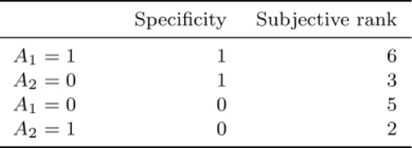
In practice, a user often performs top-k mining with respect to an objective quality measure, and with additional constraints to restrict the results. Here, we assume that the user decides to mine all subgroups consisting of a single condition and rank them according to Specif icity. The resulting subgroups and ranking is shown in Table 3. The obtained ranking does clearly not match our user’s desired, subjective ranking. Without our framework, this would be the end result and the user would either have to be happy with the results, or tune the algorithm param-eters based on these results. The former is unsatisfactory, while the latter is hard: what other interestingness measure and parameters should we use to obtain more interesting patterns?
Table 3. Initial subgroups obtained by min-ing top patterns w.r.t. Specif icity, limited to patterns consisting of a single condition.
Specificity Subjective rank
A1= 1 1 6
A2= 0 1 3
A1= 0 0 5
A2= 1 0 2
The goal of our interactive pattern mining framework is to assist the user in data exploration. To this end, the algorithm proposes the user to inspect and com-pare small sets of subgroups. In this example, let us assume that the subgroups
provide the user with the tools necessary to inspect and understand the patterns (for example, by means of data visualization); these issues are actively researched in the fields of human-computer interaction and visual analytics.
With the help of these tools, the user gains an understanding of the current patterns, the data, and of her interests, which enables her to provide feedback. In this case, the ranking A2= 0 A1 = 0 A1= 1 would be given, as this coincides
with the subjective, implicit ranking we assume the user to have. This implies that A2= 0 is deemed subjectively most interesting, whileA1 = 1 is the least interesting
of the three.
Next, the algorithm uses the obtained feedback to learn a (subjective) pattern ranking function. To be able to use existing learning algorithms for this purpose, patterns are represented as numeric feature vectors (the details are explained in Section 6). Then, Ranking SVM is applied to learn a linear ranking function h(~p) = w~ ·~p, i.e., a vector of pattern feature weights defining a ranking function that is consistent with the user feedback.
To improve the ranking function, the interaction and learning steps can be re-peated a number of times. In our example, the algorithm queries another set of sub-groups {A2 = 0;A2 = 1;A1= 1}, obtains the ranking A2 = 1 A2 = 0 A1 = 1
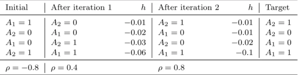
as feedback, and learns a new weight vector for h. The e↵ect of interaction and learning is shown in Table 4. After two iterations, the learned ranking is almost identical to the desired target ranking, and certainly much better than the initial ranking based on specificity. This is also reflected by Spearman’s rank correlation coefficients between the obtained and target rankings, indicated by⇢.
This concludes one full iteration of the mine, interact, and learn loop, after which the whole procedure can be repeated. The second loop is executed as the first, except that the learned ranking function is now used to mine and rank patterns.
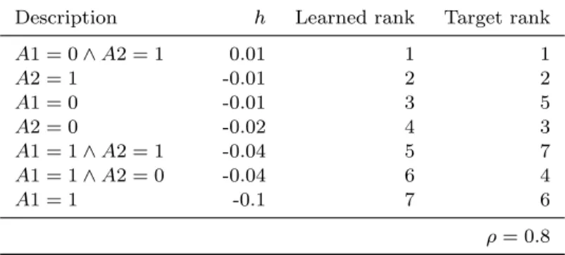
For this toy example, we evaluate the generalization capacity of the learned ranking function by applying it to the complete set of subgroups from Table 2. The results are presented in Table 5. We observe that the learned ranking function generalizes very well: when the subgroups are sorted according to this function, the resulting ranks are very close to those of the desired target ranking. In other words, the learned ranking is highly correlated with the target ranking, indicated
Table 4. Learning a desired target ranking from user input. Each iteration of feedback and learning improves the approximation of the target ranking. h
denotes the absolute score assigned by the ranking function, ⇢ is the Spear-man’s rank correlation coefficient between the indicated and target rankings.
Initial After iteration 1 h After iteration 2 h Target
A1 = 1 A2= 0 0.01 A2 = 1 0.01 A2= 1
A2 = 0 A1= 0 0.02 A1 = 0 0.01 A2= 0
A1 = 0 A2= 1 0.03 A2 = 0 0.02 A1= 0
A2 = 1 A1= 1 0.06 A1 = 1 0.1 A1= 1 ⇢= 0.8 ⇢= 0.4 ⇢= 0.8
Table 5. Generalization capacity of the learned ranking func-tion. All subgroups from Table 2 are ranked according to h.
Description h Learned rank Target rank
A1 = 0^A2 = 1 0.01 1 1 A2 = 1 -0.01 2 2 A1 = 0 -0.01 3 5 A2 = 0 -0.02 4 3 A1 = 1^A2 = 1 -0.04 5 7 A1 = 1^A2 = 0 -0.04 6 4 A1 = 1 -0.1 7 6 ⇢= 0.8
by a high correlation coefficient of ⇢ = 0.8. This implies that if h were used as interestingness measure in top-k mining, subjectively more interesting subgroups would be discovered.
In the following sections, we formalize the problem and describe the algorithms required to implement the proposed workflow, i.e., we discuss techniques for learning rankings, query selection methods, and feature representations for patterns.
5. Interactive learning of pattern rankings
We now introduce the formal definition of the pattern ranking learning task as well as algorithms for solving this task.
5.1. Learning pattern rankings
The pattern ranking task is formally defined as follows. Recall that L denotes the pattern language, that is, the universal set of all possible patterns. We will assume that there is an unknown, user-specific target rankingR⇤, that is, a total order over L. We shall write p q when p is preferred over q according to R⇤. The goal of learning will be to learn an approximation ˆR of R⇤ on the basis of the feedback provided by the user. We make the following assumptions:
The feedback takes the form of example rankings f = pf1 . . . pfn; these
are total strict orders over subsets of L. Feedback will be obtained through interaction with the user.
Each hypothesis h(in the hypothesis space H) is a ranking functionh that maps descriptions of patterns to real values and defines a ranking as follows: pi h pj
if and only if h(pi)> h(pj).
Each pattern p2 Lwill be represented by a feature vector ~p= [x1, . . . , xm].
The goal is to learn an approximation ˆRof the target rankingR⇤ that minimizes the loss function, on the basis of a set of examples F (a set of example rankings) provided by the user. Note that there is not necessarily a hypothesis h⇤ 2 H that correctly represents the unknown target ranking R⇤. This depends both on the hypothesis space H considered and the specific target ranking.
Algorithm 1 Active Preference Learning for Pattern Ranking
Input: Dataset D, ranked collection of patterns P Output: Ranking function h for patterns over D
1: F =;, h=SourceRanking(P) 2: P V =ConvertT oV ectors(P,D) 3: repeat 4: q=SelectQuery(P V, h) 5: F =F [GetF eedback(q) 6: h=LearnRankingF unction(P V, F) 7: until Stopping criterion is met
8: return h
The pattern ranking task as just defined can be seen as an instance of object ranking, for which various types of loss functions and learning algorithms have been described. Two principal categories of object ranking techniques are pairwise and
listwise methods.
Pairwise algorithms treat each sample ranking as a set of corresponding ranked pairs. For example, p~1 ~p2 p~3 corresponds to {(~p1 ~p2),(~p1 ~p3),(~p2 ~p3)}.
In the pairwise setting, the loss that needs to be minimized is a function of the number of incorrectly ranked pairs in the training data:
Losspairwise( ˆR, F) = X fk2F X (~pik ~pjk)2fi L( ˆR,~pik,~pjk)
Listwise algorithms do not reduce the rankings to pairs, i.e., each sample ranking constitutes one training example. Hence, the loss function is defined over complete rankings:
Losslistwise( ˆR, F) =
X
fk2F
L( ˆR, fk)
The pattern ranking task can be solved by finding a ranking ˆR that minimizes either a pairwise or a listwise loss function. Since we will use and evaluate instances of both, we will not state a preference here.
5.2. Algorithm for learning pattern rankings
We now present a generic algorithm for learning pattern ranking functions. Algo-rithm 1 receives a collection of patterns P ⇢ L as input. The initial pattern col-lection can be mined using any standard pattern mining algorithm, and is ranked according to an objective interestingness measure. This initial ranking is referred to as the source ranking.
In order to apply preference learning, patterns are represented as vectors of numeric features (Line 2); this will be discussed in detail in Section 6.
Within the interaction and learning loop, query selection methods select sets of patterns that will be shown to the user (Line 4). Assuming that the query size is
fixed, the goal is to minimize the number of queries required to attain a certain ranking accuracy. The methods take into account factors such as the current esti-mated interestingness of a pattern, the estimation uncertainty, the diversity of the query, and/or the structure of the data.
A user provides feedback to the queries in the form of rankings (Line 5). This feedback format is computationally more expensive for a user than graded feedback, i.e., assigning scores from a predefined scale. However, we argue that it has two advantages. First, it requires neither a deep understanding of the scale by a user, nor a thorough scale calibration. Second, graded feedback can be converted to the ordered format, albeit at a cost of reduced granularity.
The ranked queries are then used as training data for an object ranking algo-rithm. When the pairwise loss function is used, the problem is similar to classifica-tion. In fact, many pairwise algorithms are extensions of classification algorithms, e.g.,Ranking SVM14,RankBoost11, orRankNet6. Moreover, Stochastic
Coor-dinate Descent (SCD) for logistic-loss23 can be easily adapted to perform pairwise preference learning.
Listwise algorithms are designed specifically for the object ranking task. For example, ListNet7 uses neural networks and gradient descent to minimize the
loss function based on the probabilistic model of permutations. We evaluate the performance of various object ranking algorithms for pattern ranking in Section 7. The interaction and learning loop stops when a certain stopping criterion is met (Line 7). Such criteria can consider marginal e↵ects of additional queries on the learned ranking or limit the maximal user e↵ort. Alternatively, the user can manually stop the algorithm, as soon as she considers her information need satisfied. In the experiments, we stop the learning after a fixed number of iterations.
5.3. Active learning techniques
Active preference learning is a challenging problem. Selecting an optimal query is NP-hard2, therefore in most cases exact query selection methods are
computation-ally too expensive to be used in interactive settings. Consequently, heuristic methods are commonly used.
Query selection methods balance exploration of the pattern space with exploita-tion of available preference feedback. In the context of pattern mining, the source ranking is a strong starting point. The common method to ensure sufficient explo-ration is to maintain diversity among queried objects. We consider two categories of heuristics: greedy heuristics inspired by methods from information retrieval (IR), which explicitly take objective quality measures into account, and uncertainty-based heuristics specific to the Ranking SVM learner.
IR-inspired heuristics IR-inspired heuristics were initially developed in the con-text of improving search engines, hence they inherently aim at identifying a small number of top-ranking objects (documents). These greedy heuristics rely on the
availability of an objective quality measure (relevance). The query selection process always starts from a set including the currently top-ranked pattern and proceeds with greedily selecting patterns that maximize the heuristic. Let pdenote a candi-date pattern, andq the current (incomplete) query.
When applying these heuristics, we start from the raw values of the source pattern interestingness measure ', and progressively interpolate the values of the learned ranking function in order to take into account the current estimation of the target ranking:
Quality(p) =µ h(p) + (1 µ) '(p),
where µ is an interpolation parameter and his the learned ranking function.
MMR (Maximal Marginal Relevance)24 aims to select a high-quality pattern that
is dissimilar from already selected patterns. Dissimilarity is defined as the minimal distance to an already selected pattern, e.g., the Euclidean distance between pattern vectors. The parameter ↵2 [0; 1] is a quality-diversity trade-o↵parameter.
M M R(p, q) =↵ Quality(p) + (1 ↵) Diversity(p, q) where Diversity(p, q) = min
p02qdist(p, p
0)
RDD (Relevance, Diversity, and Density)32 exploits the structure in P by adding
a density term. The intuition behind this approach is that querying patterns from dense regions provides more information about preferences. Density of a region around a pattern is quantified as the average distance to all other patterns.
RDD(p, q) =↵ Quality(p) + Density(p,P) + +(1 ↵ ) Diversity(p, q) where Density(p,P) = 1 |P| X p02P dist(p, p0)
MMR and RDD only maintain local diversity, i.e., diversity within the current query. We aim to exploit global diversity, i.e., diversity between the queries, by introducing a new heuristic GlobalMMR. It is an extension of MMR, where the diversity term is redefined as Diversity(p, Q) = min
p02Qdist(p, p
0), where Q =
q[ S
fi2F
fi is the union of all queries, including the current incomplete one.
In all computations, values of the quality measure, the learned ranking function, and the distance measure are normalized to the range [0; 1]. For the quality measure and the learned ranking function, the minimal and the maximal values over P are used as range limits. For distance, the upper limit is estimated by the diameter of the object set, i.e., max
pi,pj2Pdist(pi, pj).
Uncertainty-based heuristics SVMBatch, presented in Algorithm 2, is a straightforward extension of the batch query selection method for classification SVMs by Brinker5. This method aims at selecting a diverse set of examples with
Algorithm 2 Batch query selection forRanking SVM
Input: Pattern vectorsP V, weights w, query size k, trade-o↵ , pruning parame-terminlen
1: q ;, P airs ;
2: for all pi, pj 2 P V do .Generate candidate pairs
3: Pij = pi pj
4: if dist(Pij, w) 1^||Pij|| minlen then 5: P airs P airs[Pij
6: repeat .Greedily select a diverse set of uncertain pairs
7: Pij⇤ = arg min P2P airs ⇥ dist(P, w) + (1 )⇥ max qi,qj2q cos(P, Qij) 8: q q[ p⇤i, p⇤j 9: until|q|=k 10: returnq
high prediction uncertainty. Uncertainty is quantified as the distance of a candidate example to the margin, whereas diversity is quantified by maximal cosine similarity between an example and already selected examples. This method only considers examples that lie on or within the margins.
In case of pairwise preferences, an individual example is apair of patterns. Pairs are explicitly represented as di↵erences between respective pattern vectors, similar to their representation in theRanking SVMformulation. The total number of can-didates is proportional to|P|2, therefore in order to reduce computational costs we introduce an additional pruning step. All pair vectorsPij for which||Pij||< minlen
are removed from the candidate set. The intuition behind this pruning technique is that pair vectors with low norms correspond to highly similar patterns, and reduc-ing uncertainty of predictreduc-ing relative positions of similar patterns is less useful for learning a general ranking. Note that the distance between a pair vector Pijand the
hyperplane is proportional to the di↵erence between values of the ranking function for pi and pj. However, the exact value has to be computed explicitly. Recently,
Qian et al.20 proposed a similar active learning heuristic targeted at Ranking SVM, where efficiency is ensured by combining locality-sensitive and uncertainty hashing.
Preliminary experiments confirmed the utility of batch querying, e.g., querying the union of the two most informative pairs yields a larger performance improvement than three consecutive queries of the single most informative pair (in both cases 6 pairs are queried). Pruning reduces the runtime and can have a positive impact on learning performance; see Section 7 for experiments.
5.4. Mining using learned ranking functions
As also demonstrated in the toy example in Section 4, the learned ranking function generalizes beyond the training data F and the input pattern set P. Hence, it can
be regarded as a general subjective interestingness measure defined over the pattern language L, for the current user and dataset D. It can be used to discover novel patterns that are likely to be interesting to the user.
A straightforward approach to accomplish this is to use the ranking function h directly as a search heuristic. In addition to h, a search algorithm needs access to the function that converts a pattern to its corresponding feature vector. Given h and the right feature representation, a search algorithm can compute subjective interestingness scores for each pattern p 2 L and hence use this as optimization criterion.
Devising a generic search algorithm for any type of pattern and ranking function h is an interesting and challenging open research problem on itself. We therefore leave this for future work and only specify an instance tailored for subgroup discov-ery in the next section.
6. Learning itemset and subgroup rankings
We now describe two instances of our proposed approach, for two types of pattern mining: (frequent) itemset mining and subgroup discovery. The key choices concern the source ranking and the pattern features. In making these choices, we aim to keep things as simple as possible, in order to avoid the necessity of data mining expertise and hence making our approach accessible to domain experts as well.
6.1. Frequent itemset mining
For itemset mining, in absence of any prior knowledge, the ranking according to frequency is the most natural choice of the source ranking. We consider the following features for itemsets:
• Attributei: a binary feature for each item; equals 1 i↵ the corresponding item belongs to the itemset.
• CoverT: a binary feature for each transaction; equals 1 i↵ the corresponding transaction is covered by the itemset.
• Frequency: a numeric feature; the frequency of the itemset.
• Length: a numeric feature; the size of the itemset, i.e.,|I|.
The total number of features depends on the dimensions of the data, and is equal to|I|+|D|+ 2.
6.2. Subgroup discovery
In case of subgroup discovery, there is more information than just frequency that can be used to start from a –potentially– better source ranking. That is, any objective subgroup interestingness measure ' can be used, e.g, Sensitivity or Specificity. A standard subgroup discovery algorithm can be used to mine the initial pattern set and corresponding source ranking.
In addition to the features described for frequent itemset mining, which can be used in almost any pattern mining setting, we consider the following features specific to subgroup discovery:
• Positive Frequency: a numeric feature; the frequency of the positive labels in the subgroup, i.e., C
1 |D1|.
• Negative Frequency: a numeric feature, the frequency of the negative labels in the subgroup, i.e., C
0 |D0|.
• Interestingness: a numeric feature; '.
Also, due to a richer pattern language, feature sets Length andAttributeA have a slightly di↵erent interpretation in case of subgroup discovery: Length is equal to the number of conditions in the description, and each attribute is still represented by a single binary feature AttributeA, even if it occurs in multiple conditions. For example, if A1andA2are numeric attributes, a subgroup A1 >1^A1 <2^A2 >0
has Length= 3,Attribute(A1) = 1, and Attribute(A2) = 1.
In order to use the learned ranking function h for mining new patterns, we employ a beam search–based subgroup discovery algorithm,DSSD27. At each level,
h is used to rank candidates in the beam; no other changes to the algorithm are necessary.
7. Experiments
In previous sections we described a framework for interactive learning of pattern ranking functions. The key research question is: “Is it possible to learn preferences over patterns, given only sample rankings as input?” We demonstrate that the answer is positive and proceed with answering the following more specific research questions:
Q1) Which ranking algorithms are most suitable for this purpose?
Q2) For which pattern types is learning feasible? If so, how much training data is required?
Q3) Which pattern features are important for learning?
Q4) Does active learning reduce the user e↵ort? Which query selection methods perform better with respect to various performance measures?
Q5) Do the learned ranking functions enable the discovery of novel interesting pat-terns when used as search heuristics?
7.1. Evaluation methodology
User feedback emulation Evaluating interactive data mining algorithms is hard, for experts are scarce, and it is virtually impossible to collect enough data for drawing reliable conclusions. In order to perform an extensive evaluation we use
an objective ranking of patterns as the target ranking. We emulate user feedback by ranking patterns using an objective interestingness measure (target measure), which is not known to the learning algorithm. We use Surprisingness for itemset mining and 2 for subgroup discovery (see Section 3 for definitions).
Performance measures Given a set of patterns P, the goal of learning rankings is two-fold: 1) to identify subjectively interesting patterns in P and 2) to learn an accurate overall ranking of P. Therefore, we use several ranking distance mea-sures to quantify learning performance. LetRP⇤ denote the target ranking ofP, ˆRP the learned ranking, and ˆRP(i) the learned rank of the i-th element in the target ranking:
1) In order to evaluate the capacity of the algorithm to identify the most inter-esting patterns in P, we consider Recall at k:
Reck =
n
i2{1,2, . . . , k} |RˆP(i)ko
2) In order to evaluate the overall ranking accuracy, we consider rank correlation and discounted error. Spearman’s rank correlation coefficient⇢is based on the sum of squared di↵erences between learned and target ranks for each element:
⇢= 1 6Ds(R⇤P,RˆP)
|P|(|P| 1) , where Ds = X
(i RˆP(i))2
Rank correlation essentially assigns equal weights to all elements, whereas Dis-counted Error DE assigns larger weights to higher-ranked elements:
DE =X|i RˆP(i)| ln(i+ 1)
We use⇢ as the primary performance measure in the exploratory experiments. Performance measures calculated for the entire ranking, such as ⇢ or DE, are less relevant if the ultimate goal is to identify top-ranking patterns. However, if the goal is to learn a search heuristic, the capacity to correctly identify low-ranked patterns is important as well. Note that reported values of DE are normalized to the range of [0,1].
In order to estimate the convergence rate of the algorithm, for each performance measure we report values of the area under performance curve (AU C) in addition to absolute values. The performance curves are constructed as follows: for each iter-ationi, the value of a performance measure afteriiterations is recorded. The larger the area, the fewer iterations are required to attain high values of the performance measure.
To quantify user e↵ort, we use the total number of distinct queried pairs CF:
CF = |{(pik, pjk) |fk 2F;pik, pjk 2fk}|. CF is equal to the number of pairwise
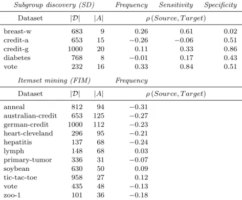
Table 6. Datasets and pattern sets used in experiments. For each dataset, source rankings of 1000 patterns were mined using various objective interestingness measures: Frequency for both itemset min-ing and subgroup discovery, and Sensitivity and Specificity for sub-group discovery. For each source ranking, Spearman’s rank correla-tion ⇢ between the source ranking and the target ranking is reported.
Setting Source rankings
Subgroup discovery (SD) Frequency Sensitivity Specificity
Dataset |D| |A| ⇢(Source, T arget)
breast-w 683 9 0.26 0.61 0.02
credit-a 653 15 0.26 0.06 0.51
credit-g 1000 20 0.11 0.33 0.86
diabetes 768 8 0.01 0.17 0.43
vote 232 16 0.33 0.84 0.51
Itemset mining (FIM) Frequency
Dataset |D| |A| ⇢(Source, T arget)
anneal 812 94 0.31 australian-credit 653 125 0.27 german-credit 1000 112 0.23 heart-cleveland 296 95 0.21 hepatitis 137 68 0.24 lymph 148 68 0.03 primary-tumor 336 31 0.07 soybean 630 50 0.09 tic-tac-toe 958 27 0.12 vote 435 48 0.13 zoo-1 101 36 0.18
Datasets For our empirical evaluation we used datasets from publicly available repositories: 11 datasets for itemset mining were taken from the CP4IM repositorya;
5 datasets for subgroup discovery were taken from the UCI repositoryb. Tuples with missing attribute values were removed from all datasets.
Source rankings The 1000 most frequent closed itemsets, ranked by their fre-quencies, were used as source rankings for experiments with itemset mining. Source subgroup rankings were mined using DSSD with the following parame-ters (see Van Leeuwen and Knobbe27 for details): minimal frequency = 0.1 |D|,
beam width = 100, maximal depth = 5. Numeric attributes were discretized on-the-fly by local binning of occurring values into 6 equal-sized bins. The cover-based beam selection heuristic was applied with the default trade-o↵ parameter settings. 10000 subgroups were mined initially, then 1000 subgroups were selected from this
ahttp://dtai.cs.kuleuven.be/CP4IM/datasets/ bhttp://archive.ics.uci.edu/ml/
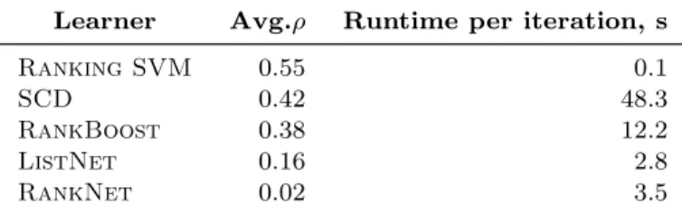
Table 7. Comparison of ranking algorithms. Ranking SVM provides the best performance in terms of av-erage rank correlation ⇢ and has the lowest runtime.
Learner Avg.⇢ Runtime per iteration, s
Ranking SVM 0.55 0.1
SCD 0.42 48.3
RankBoost 0.38 12.2
ListNet 0.16 2.8
RankNet 0.02 3.5
large set using the same selection heuristic. For each dataset, three subgroup sets were mined using one of the following subgroup interestingness measures, Sensitiv-ity, Specificity, or Frequency (essentially a non-supervised measure).
We have intentionally chosen simple source measures so that source and target rankings are substantially di↵erent, and hence the learning problem is challenging. Table 6 presents the characteristics of the datasets and corresponding pattern sets, including the initial rank correlation⇢0 between the source ranking and the target
ranking. Most source rankings by F requency are weakly or negatively correlated with the respective target rankings, whereas source rankings by supervised measures Sensitivity and Specif icity are better correlated with the target rankings by 2. In the experiments, we investigate which e↵ect this has on learning performance.
7.2. Experimental results
Q1) Comparison of ranking algorithms We first turn to comparing the learn-ing algorithms listed in Section 5:ListNet,RankBoost, andRankNetas imple-mented in theRankLiblibraryc; the standard implementation of Ranking SVMd; and our own implementation of SCD.
We use default parameter values in the implementations or values recommended in the original papers: ListNet(1500 epochs, learning rate = 0.00001, no hidden layers);RankBoost(300 training rounds, 10 threshold candidates);RankNet(100 epochs, learning rate = 0.00005, 1 hidden layer with 10 nodes); Ranking SVM(trade-o↵ C = 0.005) with a linear kernel, per recommendations of the au-thors, it is increased after each iteration, i.e. the e↵ective value is C0⇥iteration; SCD(1000 iterations, regularization parameter = 0.001).
For these experiments, random queries are used as training data. 10 patterns are selected uniformly at random (without replacement) from each source ranking and ranked by the target measure. All algorithms use the same training data. This pro-cedure is repeated 10 times for each source ranking; average values of performance measures are reported. Pattern sets are grouped by the source quality measure, and results are aggregated over all datasets. Results are shown in Table 7.
chttp://sourceforge.net/p/lemur/wiki/RankLib/
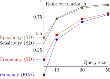
Fig. 1. Estimating the required amount of training data. Reasonably small training data of 30 ranked patterns or less suffice to attain high values of rank correlation,⇢ 0.7, Less training data is required, if the source ranking is better correlated with the target ranking, i.e. for the subgroup discovery task and SensitivityandSpecificity source rankings.
10 30 50 0.25 0.5 0.75 1 Frequency (FIM) Frequency (SD) Specificity (SD) Sensitivity (SD) Query size Rank correlation ⇢
Ranking SVM,SCD, and RankBoost are able to learn sufficiently accurate rankings, ⇢ & 0.4, which indirectly confirms feasibility of our approach. The only listwise algorithm, ListNet, does not perform well, neither does the other neural network-based algorithmRankNet. The results are consistent across pattern types. We use Ranking SVM in the following experiments, as it provides the highest performance and has the lowest runtime among the evaluated algorithms. Note that on average, one learning iteration takes approximately 0.1s, therefore in principle, this implementation can be used in a truly interactive setting.
Q2) Estimating the required amount of training data In order to estimate the amount of required training data, we select uniformly at randomSpatterns from each source ranking and use them as training data. The average rank correlation over 10 experiments is reported. Figure 1 shows the results for S 2 {0,10,30,50}, where S= 0 corresponds to the correlation between source and target rankings.
The results show that learning accurate ranking functions requires a reasonable amount of training data: querying at most 30 patterns out of 1000 allows attaining high values of ranking correlation, ⇢ 0.7. They also demonstrate the importance of prior beliefs, i.e. the choice of the source ranking: less training data is required, if the source ranking is better correlated with the target ranking, as is the case for
2 and Sensitivity or Specif icity. Furthermore, the results with the F requency
source ranking are very similar for itemsets and subgroups.
Although these results suggest that preference learning is a suitable tech-nique for ranking patterns, querying 30 patterns at once incurs considerable costs, CF = 302 = 435, which might be prohibitively large for a human user. Later, we
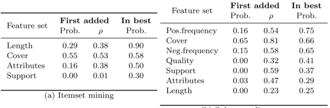
Table 8. Evaluating the importance of pattern features. We construct feature represen-tations of patterns incrementally, i.e. we start with an empty representation and add feature sets one by one, based on the improvement of rank correlation ⇢ that they enable. Features related to the target measures are considerably more likely to be in-cluded in the best feature sets, e.g. Length for Surprisingness, or Pos./Neg.frequency
for 2. For each source ranking, 10 experiments with randomly generated training data were conducted. The first two columns show the probability of a feature set be-ing added at the first iteration and the average attained value of ⇢. The rightmost columns show the probability of a feature set being included in the best feature set.
Feature set First added In best
Prob. ⇢ Prob.
Length 0.29 0.38 0.90 Cover 0.55 0.53 0.58 Attributes 0.16 0.38 0.50 Support 0.00 0.01 0.30
(a) Itemset mining
Feature set First added In best
Prob. ⇢ Prob. Pos.frequency 0.16 0.54 0.75 Cover 0.65 0.81 0.66 Neg.frequency 0.15 0.58 0.65 Quality 0.00 0.32 0.41 Support 0.00 0.59 0.37 Attributes 0.03 0.47 0.29 Length 0.00 0.23 0.25 (b) Subgroup discovery
Q3) Evaluating the importance of pattern features In order to evaluate the importance of various feature sets we performed the following procedure. Similar to the previous experiments, random subsets of P are used as the training data. For each selection of training data, we incrementally construct the pattern representa-tion. At each step the feature set that results in the largest increase of ⇢ is added to the representation. Note that feature sets such asAttribute or Cover are added as a whole, as opposed to adding features for each attribute or tuple individually. The procedure continues as long as ⇢ increases.
For each pattern type, we consider all feature sets described in Section 6. Note that all numeric features are discretized into 5 bins. The size of the training data is 30 subgroups. For each subgroup set, the training data selection procedure was performed 10 times; average values are reported. Results are shown in Table 8.
The importance of features depends on the pattern type and the target measure. For itemset mining,Lengthwas the most likely to be included in the best feature set, because long itemsets tend to have higher values ofSurprisingness.Attributes are important as well, because individual item frequencies are directly included in the formula of Surprisingness. For subgroup discovery, features that are included in the formula of 2 are likewise important, for examplePos./Neg.frequency.Cover is
important in both cases, because this feature set helps capture interactions between other features, albeit indirectly. These results also show that the learned weights are interpretable, i.e. that the algorithm not only learns accurate rankings, but can also provide explanations, which is necessary for human users.
In the remaining experiments, we use the following feature representations:
{Attributes, Cover, Length} for itemsets mining; and {Attributes, Cover, P ositiveF requency, N egativeF requency}for subgroup discovery.
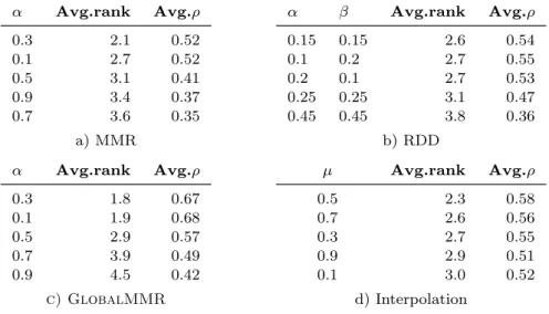
Table 9. Tuning IR-inspired active learning heuristics. For each source rank-ing, we rank parameter values according to attained values of rank cor-relation ⇢ and report average ranks across all source rankings. Lower val-ues of ↵ and , i.e., increasing diversity of selected queries, improves the performance of IR-inspired selectors. We include MMR(0.3), RDD(0.15, 0.15), and GlobalMMR(0.3) in our experiments. The e↵ect of the inter-polation coefficient µ is not substantial; we use µ = 0.5 in experiments.
↵ Avg.rank Avg.⇢ 0.3 2.1 0.52 0.1 2.7 0.52 0.5 3.1 0.41 0.9 3.4 0.37 0.7 3.6 0.35 a) MMR ↵ Avg.rank Avg.⇢ 0.3 1.8 0.67 0.1 1.9 0.68 0.5 2.9 0.57 0.7 3.9 0.49 0.9 4.5 0.42 c) GlobalMMR ↵ Avg.rank Avg.⇢ 0.15 0.15 2.6 0.54 0.1 0.2 2.7 0.55 0.2 0.1 2.7 0.53 0.25 0.25 3.1 0.47 0.45 0.45 3.8 0.36 b) RDD µ Avg.rank Avg.⇢ 0.5 2.3 0.58 0.7 2.6 0.56 0.3 2.7 0.55 0.9 2.9 0.51 0.1 3.0 0.52 d) Interpolation
Q4) Query selection We now present the comparison of query selection strate-gies. We quantify performance by average ranks of strategies with respect to various performance measures. For each source ranking, various query selectors were evalu-ated and ranked according to AUC for respective performance measures. Tied ranks are assigned the highest rank from the equivalent range. Finally, ranks for a specific query selector are averaged over all pattern sets.
Setting parameters First, we briefly describe how to set parameters of query selectors. For IR-inspired selectorsMMRandGlobalMMR, we first fix the inter-polation coefficient µ= 0.5 and vary the value of ↵ (Table 9). The larger focus on query diversity (lower values of ↵) results in the highest performance; we will use ↵= 0.3 in experiments. ForRDD, we essentially keep the same weight assigned to the diversity component (0.7) and vary the values of↵and so that↵+ = 0.3 (for completeness, we also provide results for two combinations with a lower diversity weight). The performance is slightly better than that of MMRand does not di↵er substantially for various combinations of↵ and ; we will use↵= 0.15, = 0.15 in experiments. Finally, for the chosen parameter values, we vary the value of µ. The e↵ect on performance is small; we will use µ = 0.5 in experiments. Note that we always use the Euclidean distance measure.
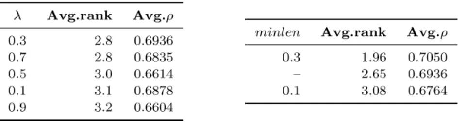
For SVMBatch, we first turn o↵ candidate set pruning and vary the values of the uncertainty weight (Table 10). In line with original findings5, the e↵ect on
performance is small; we will use = 0.3 in experiments. Then, for the chosen , we experiment with values of the pruning threshold minlen, where minlen = x
Table 10. Tuning an uncertainty-based active learning heuristic SVM-Batch. Performance of SVMBatch does not depend substantially on the uncertainty weight . Pruning a candidate set can improve per-formance. We use = 0.3 and minlen = 0.3 in experiments.
Avg.rank Avg.⇢ 0.3 2.8 0.6936 0.7 2.8 0.6835 0.5 3.0 0.6614 0.1 3.1 0.6878 0.9 3.2 0.6604
minlen Avg.rank Avg.⇢ 0.3 1.96 0.7050 – 2.65 0.6936 0.1 3.08 0.6764
denotes pruning all candidate pairs with the norm less than x·p2d and p2d is the maximal norm of a binary vector of the dimensionalityd(the dimensionality of a pattern feature vector depends on the dimensions of the dataset and the chosen feature sets). We observe that pruning can potentially improve the performance, hence we will use minlen= 0.3 in experiments. Note that larger values of minlen in certain cases can result in overly eager pruning and hence in empty candidate sets; therefore they are not reported in the table.
Comparison of query selection heuristics Following the results of previous ex-periments, we compare the following heuristics: IR-inspired selectors MMR(↵ = 0.3), RDD(↵ = 0.1, = 0.2), and GlobalMMR(↵ = 0.3) with µ = 0.5 and the Euclidean distance measure; SVMBatch( = 0.1, minlen = 0.1). A non-biased randomized strategy Random, which selects subsets of the source ranking uniformly at random, is used as a baseline. To compute the ranks of Random, for each experimental setting, 10 experiments were conducted, and median values of performance measures were used.
All experiments were conducted with 10 iterations and query size S = 5. The maximal e↵ort is thenCF = 10⇥ 52 = 100. A single query of 15 patterns has roughly
equivalent costs,CF = 152 = 105, therefore we report the median performance over
10 experiments with Random and S= 15 as a non-iterative baseline.
Table 11 presents the aggregate results regarding the performance of query se-lectors. They show that global query diversity is required to learn accurate overall rankings: methods that ensure global diversity, i.e., GlobalMMR, SVMBatch, and Random, attain the highest values of ⇢ and DE. However, active learning heuristics slightly outperform Random in terms of DE, i.e., they are more accu-rate at the top of the ranking. The performance of IR-inspired selectors,MMRand
RDD, is substantially lower, but acceptable, i.e., it is comparable to the baseline. However, they incur considerably lower costs: they query approximately two times fewer pattern pairs. Also, their recall at the top of the ranking is substantially larger than for the random query selection.
Table 12 shows results grouped by source measures. The performance of ac-tive learning strongly depends on the source ranking. For the source rankings
Table 11. Comparison of active learning heuristics. For each source ranking, heuris-tics are ranked based on the values of respective performance measures; we re-port the average ranks across all source rankings and average values of per-formance measures after 10 iterations. Perper-formance of all heuristics is compa-rable to the non-iterative baseline. Methods that ensure global diversity, Glob-alMMR and SVMBatch, result in accurate overall rankings, i.e. rank highly ac-cording to rank correlation ⇢ and discounted error DE. MMR and RDD pro-vide slightly lower performance, but at considerably lower costs CF. Iterative
ran-dom query selection performs well in terms of learning overall rankings (⇢), but is outperformed in terms of recall at the top of the ranking (Rec10 and Rec100).
Left column: average rank. Right column: average value after 10 iterations.
Selector ⇢ DE Rec10 Rec100 CF
SVMBatch 2.2 0.73 2.2 0.24 1.5 0.4 2.2 0.67 3.3 99.9 GlobalMMR 2.3 0.73 2.2 0.24 1.3 0.4 2.2 0.69 3.1 94.2 Random 3 0.74 3.3 0.26 3 0.2 3.8 0.58 3.2 100 RDD 3.5 0.64 3.4 0.32 2.2 0.3 3.2 0.56 1.6 46.2 MMR 3.7 0.63 3.5 0.32 2.3 0.3 3.1 0.58 1.4 44.1 Random(S=15) 0.64 0.32 0.1 0.48 105
highly correlated with the target ranking, i.e., the subgroup discovery task and the Sensitivity and Specif icity source rankings, active learning heuristics outperform random query selection according to most performance measures.
Q5) Generalizing to the entire pattern language Finally, we evaluate the capacity of learned ranking functions to generalize to unobserved patterns: we es-timate the target interestingness of top-k patterns according to learned ranking functions, which do not necessarily belong to the source rankingP, and compare it with the interestingness of patterns that are obtained by the search guided by the target measures directly. We use k= 1000.
For itemset mining, we first mine a complete collection of frequent itemsets at = 0.1 and rank it using Surprisingness and the learned ranking function h to obtain the top-k patterns. We restrict ourselves to the datasets that contain less than 1 million itemsets at this support threshold: primary-tumor (50040 itemsets),
soybean (27635 itemsets), tic-tac-toe (1661 itemsets), vote (49097 itemsets), and
zoo-1 (151806 itemsets).
For subgroup discovery, we useDSSDto search with 2 and its extension as de-scribed in Section 6 to search with the learned ranking functions. Search parameters were identical to the parameters used for mining the source rankings, and learning parameters were identical to the ones used in the query selection experiments.
The results confirm the generalization capacity of learned ranking functions (Table 13): median values of the target measures of top k patterns according to h increase substantially, when compared to source rankings. Maximal values are comparable to what can be achieved with direct search. Moreover, learning accurate rankings increases the magnitude of improvement. For this reason, GlobalMMR
Table 12. Comparison of active learning heuristics; results are grouped by source mea-sures. For each source ranking, heuristics are ranked based on the values of respective performance measures; we report the average ranks across all source rankings and aver-age values of performance measures after 10 iterations. Performance of query selectors depends on the source ranking. Active learning outperforms iterative random query selection both with respect to overall ranking correlation ⇢ and recall at the top of the rankingRec10, when the source ranking is correlated with the target ranking, i.e. for the subgroup discovery setting and theSensitivity orSpecif icity source rankings.
Left column: avg.rank. Right column: avg.value after 10 iterations.
Task Source Selector ⇢ Rec10
Subgroup discovery Frequency Random 1.5 0.71 3.8 0.2 GlobalMMR 2.2 0.59 1.4 0.6 SVMBatch 2.8 0.46 2.4 0.5 MMR 4 0.38 3.2 0.3 RDD 4.4 0.4 3.2 0.2 Sensitivity SVMBatch 1.2 0.94 1.6 0.8 GlobalMMR 2 0.95 2 0.8 RDD 3.6 0.85 2.8 0.6 MMR 3.6 0.89 3.4 0.6 Random 4 0.87 4.3 0.2 Specificity SVMBatch 1.2 0.93 1.8 0.8 GlobalMMR 2.2 0.91 1.4 0.9 RDD 3.4 0.86 3.2 0.7 Random 3.7 0.85 4.3 0.5 MMR 4 0.86 3 0.7
Itemset mining Frequency
GlobalMMR 2.5 0.62 2.5 0.2
SVMBatch 2.9 0.66 2.9 0.2
Random 3 0.62 3 0.1
RDD 3.2 0.55 3.2 0.1
MMR 3.5 0.52 3.5 0.1
The generalization performance is lower in the case of itemset mining, due to a source ranking that is less correlated with the target. This makes overfitting more likely; in other words, the learned ranking functions are only applicable to P, but not to the entire L. This is the case for SVMBatch: larger values of ⇢ result in lower Surprisingness of top-ranked itemsets.
Figure 2 presents a detailed view of two experiments withSVMBatch, with the datasetprimary tumor for itemset mining and the dataset credit-a and the source ranking bySpecificity. The ranking functions learned after 1, 2, 5, and 10 iterations were used in the search. The boxplots show the distribution of the target measures (Surprisingness and 2 respectively) in the set of top-1000 patterns according to the learned ranking function. They illustrate the phenomena discussed in the pre-vious paragraph. For itemset mining, overfitting results in decrease of the maximal Surprisingness after more learning iterations. Nevertheless, the median gradually increases. For subgroup discovery, the more learning iterations are performed, the more the distributions are skewed towards high values of 2. Median and maximal values are comparable to ones obtained with 2 used directly as a search heuristic.
Table 13. Evaluating generalization capacity of learned ranking functions. For each dataset, we learn a ranking function h for a number of iterations and use it to mine novel sub-groups or rank a complete collection of frequent itemsets. 'med (resp. '⇤med) denote
the ratio between the median values of the target measure ' in top 1000 patterns accord-ing to h (mined or ranked) and in the source ranking (resp. in top 1000 subgroups ac-cording to ' directly), whereas 'max and '⇤max denote the ratios between the
maxi-mal values of ' in respective sets. For each selector, we report the median values of these ratios across all datasets and source rankings. Learned ranking functions generalize beyond the source rankings, as evidenced by the increase of median target measure values ( 'med).
Learning accurate overall rankings (higher values of ⇢) improves quality of discovered pat-terns, although the e↵ect is more pronounced for subgroup discovery than for itemset mining.
Setting Selector Iterations Avg.⇢ 'med 'max '⇤med '⇤max
SD GlobalMMR 5 0.6574 1.85 1.03 0.54 0.96 10 0.7443 2.05 1.03 0.64 0.96 MMR 5 0.5952 1.73 1.02 0.34 0.94 10 0.5845 1.7 1.01 0.27 0.92 SVMBatch 5 0.6480 2.63 1.02 0.43 0.98 10 0.7567 3.29 1.02 0.68 0.96 FIM GlobalMMR 5 0.4688 2.09 0.835 0.565 0.83 10 0.6062 2.16 0.905 0.575 0.89 MMR 5 0.3494 2.215 0.87 0.655 0.835 10 0.3808 2.275 0.87 0.575 0.835 SVMBatch 5 0.4143 3.38 0.925 0.68 0.89 10 0.6318 2.735 0.84 0.54 0.805
Fig. 2. Generalization capacity of learned ranking functions. We use a ranking function learned after a certain number of iterations to mine or rank complete collections of patterns. The more learning iterations are performed, the higher the values of the target measure of the patterns discovered with the learned ranking function as a search heuristic. For subgroup discovery, the results after 10 learning iterations are comparable to the search directly guided by the target measure 2. For itemset mining, the learning is more prone to overfitting, therefore the maximal target interestingness of discovered itemsets tends to decrease. Nevertheless, the median target interestingness gradually increases.
Source 1 2 5 10 Direct Ta r g e t m e a s u r e
(a) Subgroup discovery:
credit-a, source ranking bySpecif icity
Source 1 2 5 10 Direct
(b) Itemset mining:
primary-tumor
8. Discussion
We introduced a generic algorithm for the interactive learning of pattern rankings, based on o↵-the-shelf preference learning techniques and active learning heuristics