Cross-validation in model-assisted estimation

(1)

2009

Cross-validation in model-assisted estimation

Lifeng You

Iowa State University

Follow this and additional works at:

https://lib.dr.iastate.edu/etd

Part of the

Statistics and Probability Commons

This Dissertation is brought to you for free and open access by the Iowa State University Capstones, Theses and Dissertations at Iowa State University Digital Repository. It has been accepted for inclusion in Graduate Theses and Dissertations by an authorized administrator of Iowa State University Digital Repository. For more information, please [email protected].

Recommended Citation

You, Lifeng, "Cross-validation in model-assisted estimation" (2009).

Graduate Theses and Dissertations

. 10457.

(2)

by

Lifeng You

A dissertation submitted to the graduate faculty

in partial fulfillment of the requirements for the degree of

DOCTOR OF PHILOSOPHY

Major: Statistics

Program of Study Committee:

Jean D. Opsomer, Major Professor

Michael Larsen

Huaiqing Wu

Cindy L. Yu

Helen H. Jensen

Iowa State University

Ames, Iowa

2009

(3)

DEDICATION

I would like to dedicate this thesis to my husband Lei without whose support I would

not have been able to complete this work. I would also like to thank my friends and family

for their loving guidance and financial assistance during the writing of this work.

(4)

TABLE OF CONTENTS

LIST OF TABLES . . . .

v

ACKNOWLEDGEMENTS . . . .

ix

ABSTRACT . . . .

x

CHAPTER 1. Cross-Validation in Penalized Spline Model-Assisted

Esti-mation . . . .

1

1.1

Introduction . . . .

1

1.2

Definition of the Estimator and Smoothing Parameter Selection . . . .

4

1.2.1

Definition of the Estimator . . . .

4

1.2.2

Smoothing Parameter Selection . . . .

6

1.3

Theoretical Properties . . . .

7

1.4

Simulation Results . . . .

20

1.5

Conclusion . . . .

26

CHAPTER 2. CV as Improved Variance Estimation for Model-Assisted

Estimators . . . .

28

2.1

Introduction . . . .

28

2.2

29

2.3

33

2.4

Simulation Results . . . .

46

2.5

Conclusion . . . .

53

CHAPTER 3. Shrinking for Linear Regression Estimation . . . .

55

3.1

55

(5)

3.3

73

3.4

Conclusion . . . .

78

CHAPTER 4. Model Selection for Regression Estimators . . . .

79

4.1

Definition of the Estimator . . . .

79

4.2

80

4.3

81

4.4

Conclusion . . . .

90

APPENDIX A. Technical Lemmas

. . . .

91

A.1 Lemmas I . . . .

91

A.2 Lemmas II . . . .

97

APPENDIX B. Additional Simulation Results . . . .

100

B.1 More Simulation Results in Chapter 1 . . . 100

(6)

(7)

(8)

(9)

(10)

ACKNOWLEDGEMENTS

I would like to take this opportunity to express my thanks to my major professor, Dr.

Opsomer, for his guidance, patience and support throughout this research and the writing

of this thesis. I would also like to thank my committee members for their efforts and

contributions to this work: Dr. Larsen, Dr. Wu, Dr. Yu and Dr. Jensen. I would additionally

like to thank Dr. Hofmann for her guidance throughout the initial stages of my graduate

study. Finally I would like to thank Dr. Kling and Dr. Maiti for their valuable comments

and suggestions to my research study.

(11)

ABSTRACT

Variance estimation for survey estimators that include modeling relies on approximations

that ignore the effect of fitting the models. Cross-validation (CV) criterion provides a way

to incorporate this effect. We will show 4 ways in which we explore this in this dissertation.

Penalized spline regression, as a main type of nonparametric model assisted methods, is

a common technique to improve the precision of finite population estimators. In Chapter 1,

we propose a CV based criterion to select the smoothing parameter for the penalized spline

regression estimator. The design-based asymptotic properties of the method are derived,

and simulation studies show how well it works in practice.

Regression estimator is a common technique to improve the precision of finite population

estimators by using the available auxiliary information of the population. In Chapter 2, we

propose a CV based variance estimator and compare it to other two variance estimators.

The design-based asymptotic properties of the estimator are derived, and simulation studies

show how well it works in practice.

Regression estimator works well for the cases where there is a strong linear relationship

between regressor and regressands. On the contrary, when the relationship is weak,

π

esti-mator is a good choice. In Chapter 3, a new estiesti-mator as a linear combination of those two

estimators is proposed to select between them. We introduce a CV based variance estimator

for the new proposed estimator. The design-based asymptotic properties of the estimator

are explored, and simulation studies show how well it works in practice.

In linear regression estimation, how to choose the set of control variables

x

is a difficult

practical problem. In Chapter 4, a CV criterion is introduced for choosing between

combina-tions of the

x

variables to be included in the model. The design-based asymptotic properties

of the estimator are explored, and simulation studies show how well it works in practice.

(12)

CHAPTER 1.

Cross-Validation in Penalized Spline

Model-Assisted Estimation

1.1

Introduction

In many surveys, the available auxiliary information for the population can be used to

improve the precision of design-based estimators. Thereinto ratio and regression estimators

have been used for a long time in survey estimation, e.g., Cochran (1977).

Breidt and Opsomer (2000) proposed a nonparametric model-assisted regression

esti-mator with the relationship between the variables to be any smooth function. They used

kernel-based local polynomial regression and showed that the nonparametric estimator has

the same asymptotic design properties of the parametric model-assisted estimators.

The practical properties of the estimator depend on the choice of a smoothness

tun-ing parameter, i.e., the bandwidth in local polynomial regression. In Breidt and Opsomer

(2000), the bandwidth is treated as a fixed quantity and the issue of how to best select a

bandwidth value is not addressed. In Opsomer and Miller (2005), the issue of smoothing

parameter selection for nonparametric model-assisted estimation was explored and a

sample-based criterion that could be used for this purpose was proposed. The proposed smoothing

parameter selection method was based on minimizing a type of cross-validation criterion,

suitably adjusted for the effect of the finite population setting and the survey design.

Penalized spline regression, often called P-splines, is a main type of nonparametric

model-assisted methods introduced by Eilers and Marx (1996). P-splines are flexible and can be

incorporated into a wide range of modelling contexts. Ruppert et al. (2003) gave an overview

of applications of P-splines to different settings. P-splines are also a natural candidate for

constructing nonparametric small area estimators in terms of their close connections with

(13)

linear mixed models discussed in Wand (2003).

The ability of combing nonparametric regression and mixed model regression with

P-splines was used in different contexts, e.g., Parise et al. (2001) and Coull et al. (2001). They

all provided examples of using penalized splines in the construction of mixed effect regression

models to analyze the data with random effects. In the survey context, Zheng and Little

(2003) proposed a model-based estimator for cluster sampling, where the regression model

combines a spline model with a random effect for the clusters. Opsomer et al. (2008)

pro-posed a new small area estimation approach, which combines small area random effects with

a smooth nonparametrically specified trend. The small area estimation problem could be

expressed as a mixed effect model regression by using penalized splines as the representation

for the nonparametric trend. They showed consistency of the estimator, computed its mean

squared error and provided tests for small area effects and non-linearities.

Breidt et al. (2005) proposed a class of estimators based on penalized spline regression.

Those estimators are weighted linear combinations of sample observations, and weights are

calibrated to known control totals. The estimators are design consistent and asymptotically

normal under the conditions of standard design, and they admit consistent variance

estima-tion by using design-based methods. Breidt et al. (2005) considered data-driven penalty

selection in the context of unequal probability sampling designs and showed that the

esti-mators are more efficient than parametric regression estiesti-mators when the parametric model

is incorrectly specified, while being approximately same efficient when the parametric model

specification is correct.

Modelling a regression function as a piecewise polynomial with a large number of pieces

relative to the sample size is involved in regression spline smoothing. Since the number

of possible models is so large, efficient strategies are required for choosing among them.

Wand (2000) reviewed some approaches to this problem and compared them through a

simulation study. For simplicity, Wand (2000) considered the univariate smoothing setting

with Gaussian noise and the truncated polynomial regression spline basis. Several other

approaches for knot selection exist, e.g., the TURBO algorithm in Friedman and Silverman

(1989) and its subsequent generalization, the MARS algorithm in Friedman (1991).

(14)

vari-able, and the only parameters that can be chosen to adjust are the number of knots and

the penalty parameter. Ruppert (2002) studied the effects of number of knots on the

per-formance of penalized splines. Two algorithms for the automatic selection of the number

of knots, myopic algorithm and full search algorithm, were proposed. Ruppert (2002) also

described a Demmler-Reinsch type diagonalization for computing univariate and additive

penalized spline, which is very useful for super-fast generalized cross-validation, while being

not effective for smoothing splines since large number of knots.

The choices for the number and positioning of the knots are much less crucial than the

smoothing parameter. Ruppert et al. (2003) introduced some model selection approaches,

e.g., cross-validation (CV), generalized cross-validation (GCV), Mallows’s

C

p

criterion. The

optimal amount of smoothing in penalized spline regression was investigated in Wand (1999).

In this article, a simple closed form approximation to the optimal smoothing parameter was

derived. This approach was based on the mean average squared error (MASE), which is a

mathematically measure of the global discrepancy between

m

b

and

m

. It was shown to be

a useful starting point for measuring the optimal amount of smoothing in penalized spline

regression.

In nonparametric regression one can select the smoothing parameter by minimizing a

Mean Squared Error (MSE) based criterion. For spline smoothing, the smooth estimation

can be rewritten as a Linear Mixed Model. Then Maximum Likelihood (ML) theory can

be applied to estimate the smoothing parameter as variance component. The relationship

between spline smoothing and Mixed Models was discussed in Green and Silverman (1994),

Brumback and Rice (1998) and Verbyla et al. (1999).

In Kauermann (2005), smoothing parameter selections for P-spline smoothing based on

MSE minimization and REML estimation were compared. The results for MSE minimization

method are similar to the results provided in Wand (1999). It was shown that REML-based

smoothing parameter selection is asymptotically biased towards undersmoothing, i.e., this

approach chooses a more complex model compared to the MSE method. The result accords

with classical spline smoothing, however the asymptotic arguments are different.

Different smoother is rapidly becoming more popular, which is much easier to prove

theoretical results. In this chapter, we will propose a new CV-based criterion for smoothing

(15)

parameter selection, which has almost exact expression as the criterion (9) in Opsomer and

Miller (2005) except that a penalized spline estimator is used to estimate the smooth function

instead of a local polynomial estimator in Opsomer and Miller (2005).

Section 1.2.1 will give the definition of the spline estimator. Section 1.2.2 introduces

the smoothing parameter selection method. In section 1.3 we state assumptions used in the

theoretical derivations and our main theoretical results are described. In section 1.4, we

report simulation results, which show how well the CV-based criterion works in practice.

1.2

Definition of the Estimator and Smoothing Parameter

Selection

1.2.1

Definition of the Estimator

In survey sampling, the estimation of a finite population total,

t

y

=

X

i∈U

y

i

is a problem in common. Where

U

=

{

1

,

2

, . . . , N

}

is a finite population with

N

identifiable

elements and

y

i

is a response variable for the

i

th element. A sample of population elements

s

⊂

U

is selected with probability

p

(

s

). Let

π

i

= Pr (

i

∈

s

) =

P

_s_:_i_∈_s

p

(

s

)

>

0 denote

the inclusion probability for element

i

, then the Horvitz-Thompson estimator (Horvitz and

Thompson 1952) for

t

y

is

b

t

y,HT

=

X

s

y

i

π

i

.

(1.1)

The variance of the Horvitz-Thompson estimator under the sampling design is

Var

b

t

y,HT

=

X

i∈U

X

j∈U

(

π

ij

−

π

i

π

j

)

y

i

π

i

y

j

π

j

,

(1.2)

where

π

ij

= Pr (

i

∈

s, j

∈

s

), the joint inclusion probability for elements

i, j

∈

U

.

Suppose there is auxiliary information

x

i

available for all of

U

. Then we hope to

im-prove estimation of

t

y

by using the auxiliary information. One approach to incorporate the

auxiliary information is postulating a superpopulation model, say

ξ

, which describes the

relationship between the response variable

y

and the auxiliary variable

x

.

(16)

Consider the superpopulation regression model

y

i

=

m

(

x

i

) +

ε

i

,

(1.3)

where

ε

i

are independent random variables with mean zero and variance

v

(

x

i

),

m

(

x

i

) is

a smooth function of

x

i

, and

v

(

x

i

) is smooth and strictly positive. In order to introduce

the estimator, we treat

{

(

x

i

, y

i

) :

i

∈

U

}

as a realization from the superpopulation model

(1.3). If the entire realization were observed, we could define a P-spline estimator for

m

(

·

)

as follows:

m

(

x

;

β

) =

β

0

+

β

1

x

+

. . .

+

β

q

x

q

+

K

X

k=1

β

q+k

(

x

−

κ

k

)

q₊

,

(1.4)

where (

t

)

q₊

=

t

q

if

t >

0 and 0 otherwise,

q

is the degree of the spline,

κ

1

<

· · ·

. . . < κ

K

is a

set of fixed knots and

β

= (

β

0

, . . . , β

q+K

)

T

is the coefficient vector. Typically,

q

is kept fixed

and low. If the number of knots

K

is sufficiently large, the class of functions

m

(

x

;

β

) is very

large and can approximate most smooth functions with a high degree of accuracy.

The population estimator for

β

is defined as the minimizer of

X

i∈U

(

y

i

−

m

(

x

i

;

β

))

2

+

α

K

X

k=1

β

_q2₊_k

(1.5)

for some fixed constant

α

≥

0. The smoothness of the resulting fit depends on the value of

α

, with larger values corresponding to smoother fits.

Let

X

represent the matrix with rows

x

T_i

=

1

, x

i

, . . . , x

qi

,

(

x

i

−

κ

1

)

q+

, . . . ,

(

x

i

−

κ

K

)

q+

for

i

∈

U

, and let

Y

denote the column vector of response values

y

i

for

i

∈

U

. Define a

diagonal matrix

A

_α

= diag

{

0

, . . . ,

0

, α, . . . , α

}

, which has

q

+ 1 zeros followed by

K

penalty

constant

α

. If the population

U

is fully observed, the penalized least squares estimator for

the coefficient vector of (1.4) has the ridge-regression representation:

β

_U

=

X

T

X

+

A

_α

−1

X

T

Y

.

(1.6)

Let

m

i

=

m

(

x

i

;

β

U

)

≡

x

Ti

β

U

,

i

∈

U

denote the P-spline fit obtained from this hypothetical

population fit at

x

i

. If these fitted values are known, they can be incorporated into the

survey estimation by constructing the difference estimator (S¨arndal et al. 1992, p. 221)

b

t

y,diff

=

X

U

m

i

+

X

s

y

i

−

m

i

π

i

.

(1.7)

(17)

The difference estimator is design unbiased and its design variance is

Var

b

t

y,diff

=

X

U

X

U

(

π

ij

−

π

i

π

j

)

y

i

−

m

i

π

i

y

j

−

m

j

π

j

.

(1.8)

Obviously, the efficiency of

b

t

y,diff

depends on how well the

m

i

approximates the variable

y

i

.

The estimator (1.7) is infeasible because the

m

i

cannot be calculated. However, given

a sample

s

, the

m

i

in (1.7) can be replaced by sample-based estimators, denoted by

m

b

i

and constructed as follows. Define the diagonal matrix of inverse inclusion probabilities

W

= diag

j∈U

{

1

/π

j

}

and its sample submatrix

W

s

= diag

j∈s

{

1

/π

j

}

. Similarly, let

X

s

be

the submatrix of

X

consisting of those rows for which

j

∈

s

and

Y

s

denote the column

vector of response values

y

j

for

j

∈

s

. For fixed

α

and under suitable regularity conditions,

the

π

-weighted estimator

b

β

=

X

T_s

W

s

X

s

+

A

α

−1

X

T_s

W

s

Y

s

=

G

α

Y

s

(1.9)

is a design-consistent estimator of

β

_U

in (1.6).

Define

m

b

i

=

m

x

i

,

β

b

≡

x

T

i

β

b

. Then the model-assisted P-spline estimator is defined as

b

t

y,spl

=

X

U

b

m

i

+

X

s

y

i

−

m

b

i

π

i

.

(1.10)

1.2.2

Smoothing Parameter Selection

Introducing the indicator function

I

i

= 1 if

i

∈

s

and 0 otherwise, and the indicator

vector

e

i

which is a zero vector except for an entry of one at position

i

, we can rewrite (1.10)

as

b

t

y,spl

=

X

i∈s

(

π

−_i 1

+

X

j∈U

(1

−

I

j

/π

j

)

x

Tj

G

α

e

i

)

y

i

≡

X

s

w

i(s)

y

i

,

which shows that

b

t

y,spl

is a linear estimator.

In Breidt et al. (2005), it was shown that this estimator is design consistent and

asymp-totically design unbiased. Asympasymp-totically, the design mean squared error of

b

t

y,spl

is equivalent

to the variance of the generalized difference estimator, given in (1.8),

MSE

p

b

t

y,spl

= E

p

b

t

y,spl

−

t

y

2

≈

X

i,j∈U

(

π

ij

−

π

i

π

j

)

y

i

−

m

i

π

i

y

j

−

m

j

π

j

.

(1.11)

(18)

Finally, Breidt et al. (2005) provides a design consistent and asymptotically design unbiased

estimator of MSE

p

b

t

y,spl

, as

b

V

b

t

y,spl

=

X

i,j∈s

π

ij

−

π

i

π

j

π

ij

y

i

−

m

b

i

π

i

y

j

−

m

b

j

π

j

.

(1.12)

The problem is that minimizing

V

b

t

y,spl

does not lead to the minimizer of the MSE, since

b

m

i

can be made to be close to

y

i

by letting

α

→

0.

In Opsomer and Miller (2005),

V

b

t

y,spl

is modified so that it provides a more suitable

criterion. Specifically, each estimator

m

b

i

is replaced by the “leave-one-out” estimator

m

b

(i−)

.

This estimator is readily derived by defining a modified smoothing vector

w

′_si

with elements

w

′_sij

=







wsij 1−wsii

if

j

6

=

i

0

if

i

=

j

,

where

w

sij

denotes the

j

th element of the vector

w

si

=

x

Ti

G

α

T

, and set

m

b

(_i−)

:=

P

_j_∈_s

w

′

sij

y

j

.

The modification of

V

b

t

y,spl

proposed to use is defined as

b

V

CV

b

t

y,spl

:=

X

i,j∈s

π

ij

−

π

i

π

j

π

ij

y

i

−

m

b

(i−)

π

i

y

j

−

m

b

(j−)

π

j

.

(1.13)

We will refer to

V

b

CV

b

t

y,spl

, denoted by

V

b

CV

(

α

), as the CV criterion for smoothing

parameter selection in function estimation. We will write

α

b

CV

for the minimizer of

V

b

CV

(

α

),

and use it as an estimator of

α

opt, the minimizer of MSEp

b

t

y,spl

.

1.3

Theoretical Properties

In order to prove our theoretical results, we make the following technical assumptions

(see Breidt and Opsomer (2000) and Breidt et al. (2005)). For simplicity, we will only

consider the case with the sample size, denoted by

n

N

, fixed for each

N

, and also assume

that

n

N

→ ∞

. As above,

q

,

K

and

{

κ

k

}

are fixed.

A1. (Sampling rate

n

N

−1

). As

N

→ ∞

,

n

N

−1

→

π

∈

(0

,

1).

A2. (Inclusion probabilities

π

i

and

π

j

). For all

N

, min

i∈U

π

i

≥

λ >

0, min

i,j∈U

π

ij

≥

λ

∗

>

0,

(19)

A3. Let

D

b

s

=

n_NN2

X

T s

W

s

X

s

+

A

α

, and

D

U

=

n_NN2

X

T U

X

U

+

A

α

= E

p

b

D

s

. Assume

b

D

−_s1

,

D

−_U1

exist for all

α

∈

H

α

, where

H

α

is an interval fixed between 0 and some

constant

C

α

with 0

< C

α

<

∞

.

A4. max

i∈U

|

y

i

|

< C

y

, and max

i∈U,j∈{1,...,p}

|

x

ij

|

< C

x

, where

p

= 1 +

q

+

K

is the dimension

of

x

_i

,

C

y

and

C

x

are some positive constants.

A5. Additional assumptions involving higher-order inclusion probabilities:

lim

N→∞(i,j,k

max

)∈D3,N

|

E

p

[(

I

i

−

π

i

) (

I

j

I

k

−

π

jk

)]

|

= 0

lim

N→∞(i,j,k,l

max

)∈D4,N

|

E

p

[(

I

i

I

j

−

π

ij

) (

I

k

I

l

−

π

kl

)]

|

= 0

lim

N→∞

n

N(i,j,k

max

)∈D3,N

E

p

(

I

i

−

π

i

)

2

(

I

j

−

π

j

) (

I

k

−

π

k

)

<

∞

lim

N→∞

n

2 N

max

(i,j,k,l)∈D4,N

|

E

p

[(

I

i

−

π

i

) (

I

j

−

π

j

) (

I

k

−

π

k

) (

I

l

−

π

l

)]

|

<

∞

where

D

t,N

denotes the set of all distinct

t

-tuples from

U

.

The assumption 3 ensures that

β

b

and

β

_U

exist for all

α

∈

H

α

. The assumption depends

on the knots, the penalty constant

α

, and the distribution of the

x

_i

.

The following results establish design consistency of variance estimator of

b

t

y,spl.

Theorem 1.3.1.

Let

w

sii

=

n_NN2

x

T_i

D

b

−1

s

x

i

/π

i

, and assumptions A1-A5 hold. Then, the

aux-iliary population

{

x

j

}j

_∈_U

, error population

{

ε

j

}j

_∈_U

, and sample

s

are such that

sup

α∈Hα

b

V

CV

b

t

y,spl

−

Var

b

t

y,diff

=

o

p

N

2

n

N

,

where

Var

b

t

y,diff

=

P P

_U

∆

ijyi−_π_imiyj−_π_jmj

.

Proof of Theorem

1.3.1: We write the expression as follows

b

V

CV

b

t

y,spl

=

X

i∈s

X

j∈s

∆

ij

π

ij

y

i

−

m

b

i

π

i

y

j

−

m

b

j

π

j

1

−

w

sii

1

−

w

sjj

=

X

i∈s

X

j∈s

∆

ij

π

ij

y

i

−

m

i

π

i

y

j

−

m

j

π

j

1

−

w

sii

1

−

w

sjj

+

X

i∈s

X

j∈s

∆

ij

π

ij

m

i

−

m

b

i

π

i

m

j

−

m

b

j

π

j

1

−

w

sii

1

−

w

sjj

+2

X

i∈s

X

j∈s

∆

ij

π

ij

y

i

−

m

i

π

i

m

j

−

m

b

j

π

j

1

−

w

sii

1

−

w

sjj

=

V

1

+

V

2

+ 2

V

3

.

(20)

In this expression,

V

1

=

X

i∈U

X

j∈U

∆

ij

y

i

−

m

i

π

i

y

j

−

m

j

π

j

1

−

w

sii

1

−

w

sjj

+

X

i∈U

X

j∈U

∆

ij

y

i

−

m

i

π

i

y

j

−

m

j

π

j

1

−

w

sii

1

−

w

sjj

I

i

I

j

π

ij

−

1

=

V

11

+

V

12

.

And,

V

11

=

X

i∈U

X

j∈U

∆

ij

y

i

−

m

i

π

i

y

j

−

m

j

π

j

+

X

i∈U

X

j∈U

∆

ij

y

i

−

m

i

π

i

y

j

−

m

j

π

j

1

−

w

sii

1

−

w

sjj

−

1

= Var

b

t

y,diff

+

V

₁₁∗

.

Suppose assumptions A1, A2 hold, from Lemma A.1.3 and A.1.5, we can show that

sup

α∈Hα

|

V

₁₁∗

| ≤

sup

α∈Hα

X

i∈U

|

π

i

(1

−

π

i

)

|

(

y

i

−

m

i

)

2

π

2 i

g

ii

b

D

_s

+

sup

α∈Hα

X

(i,j)∈D2,N

|

∆

ij

|

y

i

−

m

i

π

i

y

j

−

m

j

π

j

g

ij

b

D

_s

≤

λ

1

2

X

i∈U

sup

α∈Hα

max

i∈U

|

y

i

−

m

i

|

2

sup

α∈Hα

max

i,j∈U

g

ij

b

D

_s

+

1

λ

2

X

(i,j)∈D2,N

max

(i,j)∈D2,N

|

∆

ij

|

sup

α∈Hα

max

i∈U

|

y

i

−

m

i

|

2

sup

α∈Hα

max

i,j∈U

g

ij

b

D

s

=

O

(1) +

O

N

n

N

=

O

N

n

N

,

as the fact that max

i∈U

|

∆

ii

|

= max

i∈U

|

π

i

(1

−

π

i

)

| ≤

1. Rewrite

V

12

as follows,

V

12

=

X

i∈U

X

j∈U

∆

ij

y

i

−

m

i

π

i

y

j

−

m

j

π

j

I

i

I

j

π

ij

−

1

+

X

i∈U

X

j∈U

∆

ij

y

i

−

m

i

π

i

y

j

−

m

j

π

j

1

−

w

sii

1

−

w

sjj

−

1

I

i

I

j

π

ij

−

1

=

V

121

+

V

122

.

(21)

Where, E

p

[

V

121] = 0, and

Var

p

[

V

121] =

E

p

V

₁₂₁2

=

X

i,j,k,l∈U

∆

ij

∆

kl

y

i

−

m

i

π

i

y

j

−

m

j

π

j

y

k

−

m

k

π

k

y

l

−

m

l

π

l

E

p

I

i

I

j

π

ij

−

1

I

k

I

l

π

kl

−

1

Then, by assumptions A1, A2, A5 and Lemma A.1.3,

sup

α∈Hα

|

Var

p

[

V

121]

| ≤

1

λ

4

X

i,j,k,l∈U

max

i,j∈U

|

∆

ij

|

max

k,l∈U

|

∆

kl

|

sup

α∈Hα

max

i∈U

|

y

i

−

m

i

|

4

×

max

i,j,k,l∈U

E

p

I

i

I

j

π

ij

−

1

I

k

I

l

π

kl

−

1

=

2

λ

5

λ

∗

X

(i,j,k)∈D3,N

O

1

n

N

max

(i,j,k)∈D3,N

|

E

p

[(

I

i

I

j

−

π

ij

) (

I

k

−

π

k

)]

|

+

4

λ

4

λ

∗2

X

(i,j,k)∈D3,N

O

1

n

2 N

max

(i,j,k)∈D3,N

|

E

p

[(

I

i

I

j

−

π

ij

) (

I

i

I

k

−

π

ik

)]

|

+

4

λ

5

λ

∗

X

(i,j)∈D2,N

O

1

n

N

max

(i,j)∈D2,N

|

E

p

[(

I

i

I

j

−

π

ij

) (

I

i

−

π

i

)]

|

+

1

λ

6

X

i∈U

O

(1) max

i∈U

E

p

(

I

i

−

π

i

)

2

+

1

λ

4

λ

∗2

X

(i,j,k,l)∈D4,N

O

1

n

2 N

max

(i,j,k,l)∈D4,N

|

E

p

[(

I

i

I

j

−

π

ij

) (

I

k

I

l

−

π

kl

)]

|

=

o

N

3

n

N

+

O

N

3

n

2 N

+

O

N

2

n

N

+

O

(

N

) +

o

N

4

n

2 N

=

o

N

4

n

2 N

,

which implies that sup

α∈Hα

|

V

121

|

=

o

p

N2 nN

.

By assumption A2,

max

i∈U

I

i

π

i

−

1

= max

i∈U

1

,

1

π

i

−

1

≤

1

λ

,

(1.14)

and,

max

(i,j)∈D2,N

I

i

I

j

π

ij

−

1

= max

i∈U

1

,

1

π

ij

−

1

≤

λ

1

∗

,

(1.15)

(22)

then

V

122

should have the same order as

V

11∗

. Therefore, by assumptions A1, A2, Lemma

A.1.3 and A.1.5, it can be shown that

sup

α∈Hα

|

V

122

| ≤

X

i∈U

1

λ

3

sup

α∈Hα

max

i∈U

|

y

i

−

m

i

|

2

sup

α∈Hα

max

i,j∈U

g

ij

b

D

_s

+

X

(i,j)∈D2,N

1

λ

2

λ

∗ ₍_i,j

max

₎_∈_D 2,N

|

∆

ij

|

sup

α∈Hα

max

i∈U

|

y

i

−

m

i

|

2

sup

α∈Hα

max

i,j∈U

g

ij

b

D

s

=

O

(1) +

O

N

n

N

=

O

N

n

N

,

i∈U

|

∆

ii

|

= max

i∈U

|

π

i

(1

−

π

i

)

| ≤

1. Thus, it follows that

sup

α∈Hα

|

V

12

| ≤

sup

α∈Hα

|

V

121

|

+ sup

α∈Hα

|

V

122

|

=

o

p

N

2

n

N

+

O

N

n

N

=

o

p

N

2

n

N

.

Next, we will show that

sup

α∈Hα

|

V

2

|

=

o

p

N

2

n

N

.

Note

V

2

=

X

i∈U

X

j∈U

∆

ij

m

i

−

m

b

i

π

i

m

j

−

m

b

j

π

j

1

−

w

sii

1

−

w

sjj

+

X

i∈U

X

j∈U

∆

ij

m

i

−

m

b

i

π

i

m

j

−

m

b

j

π

j

1

−

w

sii

1

−

w

sjj

I

i

I

j

π

ij

−

1

=

V

21

+

V

22

.

(23)

And,

V

21

=

X

i∈U

X

j∈U

∆

ij

m

i

−

m

b

i

π

i

m

j

−

m

b

j

π

j

+

X

i∈U

X

j∈U

∆

ij

m

i

−

m

b

i

π

i

m

j

−

m

b

j

π

j

1

−

w

sii

1

−

w

sjj

−

1

=

β

b

−

β

_U

T

X

i∈U

X

j∈U

∆

ij

x

_i

π

i

x

T_j

π

j

b

β

−

β

_U

+

β

b

−

β

_U

T

X

i∈U

X

j∈U

∆

ij

x

i

π

i

x

T_j

π

j

g

ij

b

D

s

β

b

−

β

U

=

V

211

+

V

212

.

Suppose assumptions A1, A2 and A4 hold for all

α

∈

H

α

, by Lemma A.1.1, it can be shown

that

sup

α∈Hα

|

V

211

| ≤

1

λ

2

sup

α∈Hα

b

β

−

β

_U

T

X

i∈U

π

i

(1

−

π

i

)

x

i

x

Ti

sup

α∈Hα

b

β

−

β

_U

+

1

λ

2

sup

α∈Hα

b

β

−

β

_U

T

X

(i,j)∈D2,N

max

(i,j)∈D2,N

|

∆

ij

|

x

_i

x

T_j

sup

α∈Hα

b

β

−

β

_U

=

o

p

(1)

O

(

N

)

o

p

(1) +

o

p

(1)

O

N

2

n

N

o

p

(1)

=

o

p

N

2

n

N

,

and by Lemma A.1.5

sup

α∈Hα

|

V

212

| ≤

1

λ

2

sup

α∈Hα

b

β

−

β

_U

T

X

i∈U

π

_i

(1

−

π

_i

)

x

_i

x

T_i

sup

α∈Hα

max

i,j∈U

g

ij

b

D

_s

sup

α∈Hα

b

β

−

β

_U

+

1

λ

2

sup

α∈Hα

b

β

−

β

_U

T

X

(i,j)∈D2,N

max

(i,j)∈D2,N

|

∆

ij

|

x

i

x

Tj

×

sup

α∈Hα

max

i,j∈U

g

ij

b

D

s

sup

α∈Hα

b

β

−

β

_U

=

o

p

(1)

O

(1)

o

p

(1) +

o

p

(1)

O

N

n

N

o

p

(1)

=

o

p

N

n

N

,

(24)

i∈U

|

∆

ii

|

= max

i∈U

|

π

i

(1

−

π

i

)

| ≤

1. Then, it follows that

sup

α∈Hα

|

V

21

| ≤

sup

α∈Hα

|

V

211

|

+ sup

α∈Hα

|

V

212

|

=

o

p

N

2

n

N

+

o

p

N

n

N

=

o

p

N

2

n

N

.

Rewrite

V

22

as

V

22

=

X

i∈U

X

j∈U

∆

ij

m

i

−

m

b

i

π

i

m

j

−

m

b

j

π

j

I

i

I

j

π

ij

−

1

+

X

i∈U

X

j∈U

∆

ij

m

i

−

m

b

i

π

i

m

j

−

m

b

j

π

j

1

−

w

sii

1

−

w

sjj

−

1

I

i

I

j

π

ij

−

1

=

β

b

−

β

_U

T

X

i∈U

X

j∈U

∆

ij

x

i

π

i

x

T_j

π

j

I

i

I

j

π

ij

−

1

β

b

−

β

_U

+

β

b

−

β

_U

T

X

i∈U

X

j∈U

∆

ij

x

_i

π

i

x

T_j

π

j

g

ij

b

D

_s

I

i

I

j

π

ij

−

1

β

b

−

β

_U

=

V

221

+

V

222

.

By (1.14) and (1.15),

V

22

V

21. It follows that

sup

α∈Hα

|

V

22

|

=

o

p

N

2

n

N

.

Therefore, it can be shown that

sup

α∈Hα

|

V

2

| ≤

sup

α∈Hα

|

V

21

|

+ sup

α∈Hα

|

V

22

|

=

o

p

N

2

n

N

+

o

p

N

2

n

N

=

o

p

N

2

n

N

.

Finally, we will show that

sup

α∈Hα

|

V

3

|

=

o

p

N

2

n

N

.

(25)

Note

V

3

=

X

i∈U

X

j∈U

∆

ij

y

i

−

m

i

π

i

m

j

−

m

b

j

π

j

1

−

w

sii

1

−

w

sjj

+

X

i∈U

X

j∈U

∆

ij

y

i

−

m

i

π

i

m

j

−

m

b

j

π

j

1

−

w

sii

1

−

w

sjj

I

i

I

j

π

ij

−

1

=

V

31

+

V

32

,

where

V

31

=

X

i∈U

X

j∈U

∆

ij

y

i

−

m

i

π

i

m

j

−

m

b

j

π

j

+

X

i∈U

X

j∈U

∆

ij

y

i

−

m

i

π

i

m

j

−

m

b

j

π

j

1

−

w

sii

1

−

w

sjj

−

1

=

X

i∈U

X

j∈U

∆

ij

y

i

−

m

i

π

i

x

T_j

π

j

β

_U

−

β

b

+

X

i∈U

X

j∈U

∆

ij

y

i

−

m

i

π

i

x

T_j

π

j

g

ij

b

D

_s

β

_U

−

β

b

=

V

311

+

V

312

.

Suppose assumptions A1, A2 and A4 hold, from Lemma A.1.1, A.1.3 and A.1.5 we can show

that

sup

α∈Hα

|

V

311

|

=

sup

α∈Hα

X

i∈U

X

j∈U

∆

ij

y

i

−

m

i

π

i

x

T j

π

j

β

_U

−

β

b

≤

λ

1

₂

X

i∈U

sup

α∈Hα

max

i∈U

|

y

i

−

m

i

|

max

i∈U

|

x

i

|

T

sup

α∈Hα

b

β

−

β

_U

+

1

λ

2

X

(i,j)∈D2,N

max

(i,j)∈D2,N

|

∆

ij

|

sup

α∈Hα

max

i∈U

|

y

i

−

m

i|

max

j∈U

|

x

j| T

sup

α∈Hα

b

β

−

β

_U

=

O

(

N

)

o

p

(1) +

O

N

2

n

N

o

p

(1)

=

o

p

N

2

n

N

,

(26)

and,

sup

α∈Hα

|

V

312

|

=

sup

α∈Hα

X

i∈U

X

j∈U

∆

ij

y

i

−

m

i

π

i

x

T_j

π

j

g

ij

b

D

s

β

U

−

β

b

≤

λ

1

2

X

i∈U

sup

α∈Hα

max

i∈U

|

y

i

−

m

i

|

max

i∈U

|

x

i

|

T

sup

α∈Hα

max

i,j∈U

g

ij

b

D

_s

sup

α∈Hα

b

β

−

β

_U

+

1

λ

2

X

(i,j)∈D2,N

max

(i,j)∈D2,N

|

∆

ij

|

sup

α∈Hα

max

i∈U

|

y

i

−

m

i

|

max

j∈U

|

x

j

|

T

×

sup

α∈Hα

max

i,j∈U

g

ij

b

D

s

sup

α∈Hα

b

β

−

β

_U

=

O

(1)

o

p

(1) +

O

N

n

N

o

p

(1)

=

o

p

N

n

N

,

as the fact that max

i∈U

|

∆

ii

|

= max

i∈U

|

π

i

(1

−

π

i

)

| ≤

1. Thereby,

sup

α∈Hα

|

V

31

| ≤

sup

α∈Hα

|

V

311

|

+ sup

α∈Hα

|

V

312

|

=

o

p

N

2

n

N

+

o

p

N

n

N

=

o

p

N

2

n

N

.

Write

V

32

as follows

V

32

=

X

i∈U

X

j∈U

∆

ij

y

i

−

m

i

π

i

m

j

−

m

b

j

π

j

I

i

I

j

π

ij

−

1

+

X

i∈U

X

j∈U

∆

ij

y

i

−

m

i

π

i

m

j

−

m

b

j

π

j

1

−

w

sii

1

−

w

sjj

−

1

I

i

I

j

π

ij

−

1

=

X

i∈U

X

j∈U

∆

ij

y

i

−

m

i

π

i

x

T_j

π

j

I

i

I

j

π

ij

−

1

β

_U

−

β

b

+

X

i∈U

X

j∈U

∆

ij

y

i

−

m

i

π

i

x

T j

π

j

g

ij

b

D

_s

I

i

I

j

π

ij

−

1

β

_U

−

β

b

=

V

321

+

V

322

.

(27)

Similarly, from (1.14) and (1.15),

V

32

V

31. It follows that

sup

α∈Hα

|

V

3

| ≤

sup

α∈Hα

|

V

31

|

+ sup

α∈Hα

|

V

32

|

=

o

p

N

2

n

N

+

o

p

N

2

n

N

=

o

p

N

2

n

N

.

Therefore,

sup

α∈Hα

b

V

CV

b

t

y,spl

−

Var

b

t

y,diff

≤

sup

α∈Hα

|

V

11∗

|

+ sup

α∈Hα

|

V

12

|

+ sup

α∈Hα

|

V

2

|

+ 2 sup

α∈Hα

|

V

3

|

=

O

N

n

N

+

o

p

N

2

n

N

+

o

p

N

2

n

N

+ 2

o

p

N

2

n

N

=

o

p

N

2

n

N

.

Thus, the result follows.

Theorem 1.3.2.

Let assumptions A1-A5 hold. Then, the auxiliary population

{

x

j

}j

_∈_U

,

error population

{

ε

j

}j

_∈_U

, and sample

s

are such that

lim

N→∞_α

sup

_∈_H_α

1

N

MSE

p

b

t

y,spl

−

Var

b

t

y,diff

= 0

,

where

Var

b

t

y,diff

=

P P

_U

∆

ijyi−_πmi

i

yj−mj

πj

.

Proof of Theorem

1.3.2: Let

a

N

=

P

U

(

y

i

−

m

i

)

Ii πi

−

1

,

b

N

=

P

U

(

m

i

−

m

b

i

)

Ii πi

−

1

.

Then,

E

p

a

2N

=

X

i∈U

X

j∈U

∆

ij

y

i

−

m

i

π

i

y

j

−

m

j

π

j

= Var

b

t

y,diff

.

(28)

And under assumptions A1, A2, by Lemma A.1.3,

E

p

a

2_N

≤

1

λ

2

X

i∈U

max

i∈U

|

π

i

(1

−

π

i

)

|

sup

α∈Hα

max

i∈U

|

y

i

−

m

i

|

2

+

1

λ

2

X

(i,j)∈D2,N

max

(i,j)∈D2,N

|

∆

ij

|

sup

α∈Hα

max

i∈U

|

y

i

−

m

i

|

2

=

O

(

N

) +

O

N

2

n

N

=

O

N

2

n

N

,

i∈U

|

∆

ii

|

= max

i∈U

|

π

i

(1

−

π

i

)

| ≤

1. Then it follows that

sup

α∈Hα

1

N

E

p

a

2N

=

O

N

n

N

.

(29)

Let

b

k

denote the

k

th element of

β

b

−

β

U

, from assumptions A1, A2, A4 and A5, by

Lemma A.1.2 we can show that

E

p

b

2N

=

E

p





X

(i,j)∈U

X

k,l∈{1,...,p}

x

ik

x

jl

b

k

b

l

I

i

π

i

−

1

I

j

π

j

−

1





≤

X

k,l∈{1,...,p}

q

E

p

[

b

2k

b

2l

]

v

u

t

E

p













X

(i,j)∈U

x

ik

x

jl

I

i

π

i

−

1

I

j

π

j

−

1







2







≤

X

k,l∈{1,...,p}

1

λ

2

r

sup

α∈Hα

max

k∈{1,...,p}

E

p

[

b

4 k

]







v

u

t

X

i∈U

max

i∈U,k∈{1,...,p}

|

x

ik

|

4

max

i∈U

E

p

h

(

I

i

−

π

i

)

4

i

+

v

u

t

X

(i,j)∈D2,N

max

i∈U,k∈{1,...,p}

|

x

ik

|

4

max

(i,j)∈D2,N

E

p

h

(

I

i

−

π

i

)

2

(

I

j

−

π

j

)

2

i

+

v

u

t

X

(i,j)∈D2,N

max

i∈U,k∈{1,...,p}

|

x

ik

|

4

max

(i,j)∈D2,N

E

p

h

(

I

i

−

π

i

)

3

(

I

j

−

π

j

)

i

+

v

u

t

X

(i,j,i′)∈D3,N

max

i∈U,k∈{1,...,p}

|

x

ik

|

4

max

(i,j,i′)∈D3,N

E

p

h

(

I

i

−

π

i

)

2

(

I

j

−

π

j

) (

I

i′

−

π

_i′

)

i

+

v

u

t

X

(i,j,i′,j′)∈D4,N

max

i∈U,k∈{1,...,p}

|

x

ik

|

4

×

r

max

(i,j,i′,j′)∈D4,N

|

E

p

[(

I

i

−

π

i

) (

I

j

−

π

j

) (

I

i′

−

π

i′

) (

I

j′

−

π

j′

)]

|

)

=

O

1

n

N

O

√

N

+

O

1

n

N

O

(

N

) +

O

1

n

N

O

(

N

) +

O

1

n

N

O

N

3/2

√

n

N

+

O

1

n

N

O

N

2

n

N

=

o

N

2

n

N

,

which implies that

sup

α∈Hα

1

N

E

p

b

2_N

=

o

N

n

N

,

and,

sup

α∈Hα

1

N

E

p

[

|

a

N

b

N

|

]

≤

s

sup

α∈Hα

1

N

E

p

[

a

2 N

] sup

α∈Hα

1

N

E

p

[

b

2 N

]

=

s

O

N

n

N

o

N

n

N

=

o

N

n

N

.

(30)

Rewrite MSE

p

b

t

y,spl

as follows,

MSE

p

b

t

y,spl

= E

p

h

b

t

y,spl

−

t

y

2

i

= E

p





X

i∈U

b

m

i

+

X

i∈s

y

i

−

m

b

i

π

i

−

X

i∈U

y

i

!2





= E

p





X

i∈U

(

y

i

−

m

b

i

)

I

i

π

i

−

1

!

2





= E

p





X

i∈U

(

y

i

−

m

i

+

m

i

−

m

b

i

)

I

i

π

i

−

1

!

2





= E

p

(

a

N

+

b

N

)

2

= E

p

a

2N

+ E

p

b

2N

+ 2E

p

[

a

N

b

N

]

.

Then,

sup

α∈Hα

1

N

MSE

p

b

t

y,spl

−

Var

b

t

y,diff

=

sup

α∈Hα

1

N

MSE

p

b

t

y,spl

−

E

p

a

2_N

≤

sup

α∈Hα

1

N

E

p

b

2N

+ 2 sup

α∈Hα

1

N

|

E

p

[

a

N

b

N

]

|

≤

sup

α∈Hα

1

N

E

p

b

2_N

+ 2 sup

α∈Hα

1

N

E

p

[

|

a

N

b

N

|

]

=

o

N

n

N

+

o

N

n

N

=

o

N

n

N

.

Therefore the result follows.

Corollary 1.3.1.

Let assumptions A1-A5 hold. Then, the auxiliary population

{

x

j

}j

_∈_U

,

error population

{

ε

j

}j

_∈_U

, and sample

s

are such that

sup

α∈Hα

b

V

CV

b

t

y,spl

−

MSE

p

b

t

y,spl

=

o

p

N

2

n

N

.

Thereby the theory derived above for the P-spline estimator shows that it is possible to use

b

V

CV

b

t

y,spl

, denoted by

V

b

CV

(

α

), as an asymptotically equivalent criterion to MSE

p

b

t

y,spl

,

denoted by MSE

p

(

α

), for selecting an optimal smoothing parameter

α

opt

. In section 1.4, we

will evaluate how well this selection criterion works.

(31)

1.4

Simulation Results

In this section, we follow Opsomer and Miller (2005) in the design of a simulation study.

A random population of

N

= 1000 values of

x

is generated from the uniform distribution on

[0

,

1], and 1000 values for the errors

ε

are drawn from

N

(0

,

1). This one error population is

used for all simulations, up to multiplication by

σ

. Eight populations of

y

are generated as

follows:

y

il

=

m

l

(

x

i

) +

ε

i

1

≤

i

≤

1000

,

1

≤

l

≤

8

,

where

{

m

l

}

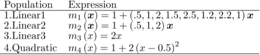
8l=1

are predefined functions given in the Table 1.1. The finite population

quan-tities of interest are

t

y

=

P1000

_i₌₁

y

il

for each

l

.

Population

Expression

1.Linear

m

1

(

x

) = 2

x

2.Quadratic

m

2

(

x

) = 1 + 2 (

x

−

0

.

5)

2

3.Bump

m

3

(

x

) = 2

x

+ exp

−

200 (

x

−

0

.

5)

2

4.Jump

m

4

(

x

) = 2

xI

{x≤0.65}

+ 0

.

65

I

{x>0.65}

5.Normal CDF

m

5

(

x

) = Φ (1

.

5

−

2

x

), where Φ is the standard normal cdf

6.Exponential

m

6

(

x

) = exp (

−

8

x

)

7.Slow sine

m

7

(

x

) = 2 + sin (2

πx

)

8.Fast sine

m

8

(

x

) = 2 + sin (8

πx

)

Table 1.1 Eight population mean functions.

The samples are drawn by one of two designs, simple random sampling without

re-placement (SI) or stratified simple random sampling without rere-placement (STSI). For each

simulation run,

M

= 1000 samples are drawn from

{

(

x

i

, y

i

)

}

. For each sample, we compute

the estimator

b

t

y,spl

in equation (1.10) for

α

opt

and

α

b

CV. Referring to Opsomer and Miller

(2005), the optimal smoothing parameters

α

opt

for each population are not sample-based. We

compute them by minimizing a simulation-based approximation to the function MSE

p

(

α

),

which is constructed by simulating repeated samples from these populations for a grid of

smoothing parameters over the interval [0

.

0001

,

10], and finding the functions MSE

p

(

α

) by

averaging over these simulations.

(32)

implemented in R, which uses expression:

b

V

CV

(

α

) :=

X

i,j∈s

π

ij

−

π

i

π

j

π

ij

y

i

−

m

b

(i−)

π

i

y

j

−

m

b

(j−)

π

j

,

the same expression as (1.13). A simulation run is determined by sample size

n

, error variance

σ

2

, and degree of the spline regression

q

. For the design of simple random sampling without

replacement, simulations are done for

n

∈ {

100

,

200

,

500

}

,

σ

2

∈ {

₀

.

01

,

₀

.

16

}

,

q

∈ {

1

}

. The

design of stratified simple random sampling without replacement uses 4 strata with each

stratum containing 250 elements, and the stratification of the strata is based on a random

variable

z

i

and ratio

r

. First, we generate

v

i

from a standard normal distribution

N

(0

, σ

v2

)

with

σ

2

v

satisfying

r

=

σ

2

σ2₊_σ2

v

. Then

z

i

’s are derived as follows:

z

i

=











v

i

+

ε

i

if 0

< r <

1

v

i

if

r

= 0, where

σ

v2

= 1

ε

i

if

r

= 1

.

After sorting by

z

i

(

i

= 1

, . . . , N

), the population is separated into 4 strata with boundaries

given by equally-spaced quantiles of

z

. Then, simulations are conducted with the stratum

sample sizes

{

(15

,

20

,

30

,

35)

,

(30

,

40

,

60

,

70)

,

(75

,

100

,

150

,

175)

}

,

r

∈ {

0

,

0

.

25

,

0

.

5

,

0

.

75

,

1

}

,

σ

2

∈ {

₀

.

01

,

₀

.

16

}

, and

q

= 1. Thus, the strata have different sampling rates with the

inclusion probability correlated with the model error.

As mentioned in Breidt et al. (2005), for

m

1

and

m

2, the models are polynomial; the

remaining mean functions are representatives with various departures from the polynomial

model. The mean function

m

3

is mostly linear over its range, except that there is a ‘bump’

for a small portion of the range of

x

k

. Function

m

4

is not a smooth function. The sigmoidal

function

m

5

is the cumulative distribution function, and

m

6

is an exponential curve. The

function

m

7

is a sinusoid completing one full cycle on [0

,

1], while

m

8

completes four full

cycles.

Since the true

α

opt

in the case with model correctly specified increases to infinity, for

simplicity, we restrict the range for searching the minimums of

α

opt

and

α

b

CV

within (0

,

10].

(33)

Population

σ

n

α

b

CV

MSE

αbCV

α

opt

MSE

αopt

1.Linear

0.1

100

8.864

90.890

10.000

89.994

0.1

200

9.121

33.828

10.000

33.800

0.1

500

9.499

9.748

10.000

9.734

0.4

100

8.864

1454.234

10.000

1439.899

0.4

200

9.121

541.251

10.000

540.804

0.4

500

9.499

155.972

10.000

155.738

2.Quadratic

0.1

100

1.668

92.636

1.385

91.601

0.1

200

1.697

34.125

1.385

33.981

0.1

500

1.102

9.749

0.774

9.742

0.4

100

7.534

1464.405

7.925

1446.792

0.4

200

7.956

543.012

4.977

541.553

0.4

500

6.030

156.101

2.783

155.799

3.Bump

0.1

100

0.004

107.197

0.003

105.423

0.1

200

0.004

37.898

0.003

37.739

0.1

500

0.003

10.044

0.003

10.022

0.4

100

0.173

1603.633

0.027

1547.149

0.4

200

0.037

582.408

0.027

581.066

0.4

500

0.016

159.168

0.015

158.539

4.Jump

0.1

100

0.005

124.059

0.003

120.596

0.1

200

0.001

43.385

0.002

42.829

0.1

500

0.000

10.987

0.001

10.921

0.4

100

1.698

1555.201

0.085

1525.090

0.4

200

0.368

578.733

0.171

567.463

0.4

500

0.023

158.539

0.048

156.861

5.Normal CDF

0.1

100

8.290

90.999

10.000

90.057

0.1

200

8.503

33.892

10.000

33.784

0.1

500

7.753

9.723

10.000

9.691

0.4

100

8.858

1455.499

10.000

1439.309

0.4

200

9.161

541.070

10.000

540.494

0.4

500

9.528

155.744

10.000

155.516

6.Exponential

0.1

100

0.158

95.709

0.048

94.708

0.1

200

0.111

35.334

0.152

34.845

0.1

500

0.043

9.914

0.027

9.889

0.4

100

4.306

1486.481

1.963

1472.820

0.4

200

2.908

549.327

1.556

544.119

0.4

500

1.069

157.463

0.215

156.945

7.Slow sine

0.1

100

0.094

94.886

0.076

93.751

0.1

200

0.103

35.249

0.121

35.026

0.1

500

0.068

9.735

0.171

9.674

0.4

100

0.408

1492.331

0.343

1475.090

0.4

200

0.436

551.640

0.546

549.310

0.4

500

0.293

155.513

0.689

154.893

Continued. . .

(34)

Population

σ

n

α

b

CV

MSE

αbCV

α

opt

MSE

αopt

8.Fast sine

0.1

100

0.001

160.854

0.001

155.795

0.1

200

0.001

42.423

0.001

41.988

0.1

500

0.001

10.692

0.001

10.654

0.4

100

0.004

1717.777

0.003

1690.978

0.4

200

0.004

611.102

0.003

607.835

0.4

500

0.003

160.394

0.005

159.522

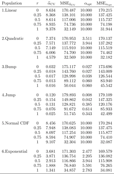
Table 1.2:

CV smoothing parameters

α

b

CV

and optimal

smoothing parameters

α

opt

with their corresponding MSEs

based on 1000 replications of simple random sampling from

all populations of size

N

= 1000.

Table 1.2 shows the cross-validation smoothing parameters

α

b

CV

and the optimal

smooth-ing parameters

α

opt

for linear spline regression under SI simulation runs. Apparently, in

agreement with

α

opt,

α

b

CV

varies widely across functions. CV and optimal smoothing

param-eters are generally an increasing function of the closeness of the relationship between

y

and

x

(as measured by

σ

2

). The difference between CV and optimal smoothing parameters is

generally a decreasing function of the sample size.

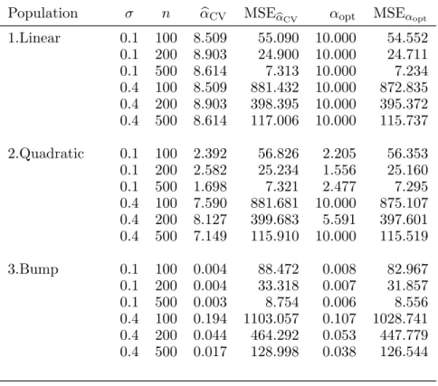
Population

σ

n

α

b

CV

MSE

αbCV

α

opt

MSE

αopt

1.Linear

0.1

100

8.509

55.090

10.000

54.552

0.1

200

8.903

24.900

10.000

24.711

0.1

500

8.614

7.313

10.000

7.234

0.4

100

8.509

881.432

10.000

872.835

0.4

<