Density Deconvolution with Laplace Errors and Unknown Variance

Density Deconvolution with

Laplace Errors and Unknown

Variance

Jun Cai, William C. Horrace, and Christopher F.

Parmeter

Paper No. 225

March 2020

CENTER FOR POLICY RESEARCH – Summer 2020

Leonard M. Lopoo, Director

Professor of Public Administration and International Affairs (PAIA) Associate Directors

Margaret Austin

Associate Director, Budget and Administration John Yinger

Trustee Professor of Economics (ECON) and Public Administration and International Affairs (PAIA) Associate Director, Center for Policy Research

SENIOR RESEARCH ASSOCIATES

Badi Baltagi, ECON Robert Bifulco, PAIA Leonard Burman, PAIA Carmen Carrión-Flores, ECON Alfonso Flores-Lagunes, ECON Sarah Hamersma, PAIA

Madonna Harrington Meyer, SOC Colleen Heflin, PAIA

William Horrace, ECON Yilin Hou, PAIA

Hugo Jales, ECON

Jeffrey Kubik, ECON Yoonseok Lee, ECON Amy Lutz, SOC Yingyi Ma, SOC

Katherine Michelmore, PAIA Jerry Miner, ECON

Shannon Monnat, SOC Jan Ondrich, ECON David Popp, PAIA Stuart Rosenthal, ECON Michah Rothbart, PAIA

Alexander Rothenberg, ECON Rebecca Schewe, SOC

Amy Ellen Schwartz, PAIA/ECON Ying Shi, PAIA

Saba Siddiki, PAIA Perry Singleton, ECON Yulong Wang, ECON Peter Wilcoxen, PAIA Maria Zhu, ECON

GRADUATE ASSOCIATES

Rhea Acuña, PAIA

Mariah Brennan, SOC. SCI. Ziqiao Chen, PAIA

Yoon Jung Choi, PAIA Dahae Choo, ECON Stephanie Coffey, PAIA Giuseppe Germinario, ECON Myriam Gregoire-Zawilski, PAIA Jeehee Han, PAIA

Mary Helander, SOC. SCI. Hyoung Kwon, PAIA

Mattie Mackenzie-Liu, PAIA Maeve Maloney, ECON

Austin McNeill Brown, SOC. SCI. Qasim Mehdi, PAIA

Claire Pendergrast, SOC Krushna Ranaware, SOC Christopher Rick, PAIA

Huong Tran, ECON Joaquin Urrego, ECON Yao Wang, ECON Yi Yang, ECON

Xiaoyan Zhang, Human Dev. Bo Zheng, PAIA

Dongmei Zuo, SOC. SCI.

STAFF

Joseph Boskovski, Manager, Maxwell X Lab Katrina Fiacchi, Administrative Specialist

Michelle Kincaid, Senior Associate, Maxwell X Lab

Candi Patterson, Computer Consultant Samantha Trajkovski, Postdoctoral Scholar Laura Walsh, Administrative Assistant

Abstract

We consider density deconvolution with zero-mean Laplace noise in the context of an error component regression model. We adapt the minimax deconvolution methods of Meister (2006) to allow estimation of the unknown noise variance. We propose a semi-uniformly consistent estimator for an ordinary-smooth target density and a modified “variance truncation device" for the unknown noise variance. We provide a simulation study and practical guidance for the choice of smoothness parameters of the ordinary-smooth target density. We apply restricted versions of our estimator to a stochastic frontier model of US banks and to a measurement error model of daily saturated fat intake.

JEL No.: C12, C14, C44, D24

Keywords:

Authors

:

[email protected]; William C. Horrace, Department of Economics, Center for Policy Research, Syracuse University, [email protected]; Christopher F. Parmeter, Department of Economics, University of Miami, [email protected]

1

Introduction

Deconvolution uses kernel techniques to estimate the density (thetarget density) of a random variable (u) in the presence of an independent and additive noise term (v). Most deconvolu-tion estimators are for a random cross-secdeconvolu-tion of observadeconvolu-tions from a noisy random variable (i.e., ε= u+v), where the noise distribution (fv) is known. If we know fv and (hence) its

characteristic function, then under regularity conditions we can calculate the empirical char-acteristic function of ε and use the Fourier inversion formula to consistently point estimate

fu. Fan (1991) shows that convergence rates for kernel deconvolution estimators depend

on the smoothness of the noise distribution, where smoothness is characterized by the tail behavior of the associated characteristic function. Specifically, ifv is from the super-smooth family (e.g., normal or Cauchy), the fastest convergence rate is logarithmic in the sample size (n), and if noise is from the ordinary-smooth family (e.g. Laplace or gamma), the fastest rate is polynomial in n.1

However, in applications (like the stochastic frontier model) it may be more practical

to assume that the noise distribution is known up to its variance. Hence, Meister (2006)

develops a semi-uniformly consistent estimator of the target density and the unknown noise variance, when the noise density is super-smooth (e.g., normal) and the target density is ordinary-smooth (e.g., gamma), which bounds the decay of the tails of its characteristic func-tion.2 _{Horrace and Parmeter (2011) adapt the estimator of Meister (2006) to the stochastic}

frontier model (Aigner et al., 1977), where the noisy random variable (ε) is appended to a lin-ear regression model,v is normally distributed, anduis ordinary-smooth and non-negative.3

1_{We give a precise definition of smoothness in the sequel. Deconvolution applications forvnormal}

(super-smooth) abound. See Stefanski and Carroll, 1990; Neumann, 1997; Johannes, 2009; Wang and Ye, 2012.

2_{Others are Butucea and Matias (2004) and Butucea, Matias, and Pouet (2008). The Meister (2006)}

estimator is uniformly consistent relative to the target distributional family but individually relative the noise distributional family. That is, consistency of the estimator does not hold uniformly over all noise distributions.

That is, for a linear production function with normally distributed (super-smooth) noise (v), we may estimate the density of technical inefficiency (u), if it belongs to the ordinary-smooth family (e.g., exponential or gamma). Unfortunately, the convergence results of Fan (1991) still apply: both the Meister (2006) and Horrace and Parmeter (2011) estimators converge at logarithmic rates. Therefore, it is natural to consider a version of Horrace and Parmeter (2011) where noise is Laplace (ordinary-smooth), so as to achieve polynomial convergence rates for estimators of the density of technical inefficiency. This is the goal of this paper.

Laplace noise is not unprecedented in the literature. Horrace and Parmeter (2018) de-velop a parametric stochastic frontier model with Laplace noise which possess useful features for ranking and selecting efficient firms.4 Meister (2004) shows that in a deconvolution prob-lem if the noise distribution is misspecified, it is always better to assume Laplace noise rather than normal, because normal noise produces infinite risk while Laplace noise produces finite risk. A similar result arises in the simulations of Horrace and Parmeter (2018) who find that the mean squared error (MSE) of the parametric stochastic frontier model is smaller with Laplace noise than with normal noise under misspecification of the noise distribution. Errors-in-variable models have recently considered Laplace errors. See Carroll et al. (2006), Koul and Song (2014), Song et al. (2016), Cao (2016) and references therein. Finally, maxi-mum likelihood estimation with Laplace errors produces the least absolute deviations (LAD) estimator, and applications of this method are plentiful in statistics, finance, engineering, and other applied sciences (see Dodge, 1987, 1992, 1997 and Dodge and Falconer, 2002).

Our aim here is to provide a complete account of Laplace kernel deconvolution and to develop a regression-based deconvolution estimator that does not require the variance of the Laplace distribution to be known. We modify the “variance truncation device” of Meister

(2006) to bound of the variance of the noise (v) with the variance of the noisy random

4_{Horrace and Parmeter do maximum likelihood estimation of the stochastic frontier model, not}

variable (ε). Target density estimation is drastically improved (in terms of convergence) with Laplace noise and is robust to misspecification of the noise distribution (per Meister, 2004). Moreover, we offer practical guidance and an adaptive procedure for selecting the smoothness parameters which are key to implementation of the proposed techniques (and which will be discussed later). This adaptive procedure is new in the literature and offers sound footing for practical use of these methods. Lastly, we apply the Laplace deconvolution estimator to two restricted versions of the model: a stochastic (cost) frontier model (SFM), where

u is restricted non-positive, and a pure deconvolution problem, where the linear regression parameters are restricted to equal zero.

The paper is organized as follows. In Section 2 we discuss the basic issues surrounding deconvolution in the regression model and introduce the modified variance truncation device under Laplace errors (noise). Section 3 derives large sample properties of the estimator under certain regularity conditions. Two extensions are considered in Section 4. Section 5 contains a variety of Monte Carlo results demonstrating the finite sample performance of the proposed estimator as well as issues pertaining to robustness of the choice of the Laplace noise. In Section 6 we provide two practical applications to illustrate the utility of the proposed methodology. Conclusions are in Section 7.

2

The Laplace Convolution Problem

Consider the error component model (ECM) in the cross sectional setting:

yj =x0jβ+uj +vj =x0jβ+εj, j = 1, . . . , n. (1)

component, and v is statistical noise. Depending on assumptions on u, the model in (1) can be a cross sectional stochastic frontier model (e.g., u ∼ Exp(σ_u2)), a linear regression with measurement error (e.g., yj = x∗jβ +vj, where x

∗

j = xj +ej, uj = β ∗ej), or a pure measurement error model (e.g., β = 0). A large statistical literature investigates the β = 0

model with known or partially-known error distribution of v (see Meister, 2009).5 _{In this}

setting, deconvolution is complicated by the fact that only cross sectional data are available. Following the literature (i.e., Fan, 1991; Meister, 2006; Horrace and Parmeter, 2011), we make the following assumptions on the random components of the model and the covariates when present.

Assumption 1. The xj, vj and uj are pairwise independent for all j = 1, . . . , n.

Let the probability densities of the error components be fv(z), fu(z) and fε(z) with

corresponding characteristic functions hv(τ), hu(τ) and hε(τ). Based on the independence

between vj and uj in Assumption 1,

hε(τ) =hv(τ)hu(τ). (2)

We restrict v to the family of Laplace densities with the following assumption.

Assumption 2. The distribution of v is a member of the Laplace family with zero mean and

unknown variance, i.e. L={Laplace(0, b) :b2 >0}.

Hence, the density of v is known up to its variance (2b2), and the characteristic function of

v is hv(τ) = (1 +b2τ2)−1, so that,

hu(τ) =

hε(τ)

hv(τ)

= (1 +b2τ2)hε(τ). (3)

5_{Neumann (1997), Johannes (2009), and Wang and Ye (2012) study deconvolution with fully unknown}

We restrict u to be ordinary-smooth (Fan, 1991) with the following assumption.

Assumption 3. Assume u is ordinary-smooth. Namely, u belongs to the family Fu =

hu :

C1|τ|−δ ≤ |hu(τ)| ≤C2|τ|−δ, f or |τ| ≥T >0 where 0< C1 < C2 and δ >1, δ 6= 2.

Assumption 3 dictates tail behavior of the characteristic function of u (smoothness of the

density of u), and positive constants C1, C2 and δ are smoothness parameters. The lower

bound, C1, and upper bound, C2, ensure the rate of decay of the tails of the characteristic

function does not approach zero too rapidly or too slowly and are needed for identification.

Constants C1 and C2 become irrelevant when T gets large. Practically speaking, we only

use the lower bound to define our variance truncation device, so only C1 is relevant to our

estimator. We assume C1 and δ to be known for now but will relax this in the sequel.6

Constantδis thesmoothness order, ensuring polynomial tail behavior of the characteristic function, and includes a wide array of nonparametric and analytical families (Horrace and Parmeter, 2011). Common families and their polynomial smoothness orders are tabulated in Table 1. For example, the Symmetric Uniform family of distributions has polynomial order

δ = 1, and the Laplace family has δ = 2. We restrict δ 6= 2 in Assumption 3 so that the

target density cannot be Laplace, allowing our estimator to appropriately assign the target

and noise distributions. That is, if u and v are both Laplace, we cannot determine which

distribution is the target and which is the noise.7 In the parlance of frontier estimation, whenδ = 2 we cannot distinguish the signal from the noise. Lettingδ = 2 does not preclude

deconvolution per se. For example, the deconvolution convolution estimator of Dattner et

al. (2011) relies on very general classes of distributions for the target and noise densities that includes the Laplace-Laplace convolution as a special case, and consistent target density estimation is achieved as long as the error variance is known. The restriction in Assumption 3

6_KnowingC

thatδ >1 does not preclude a nonparamteric family of densities in Table 1 that is arbitrarily

close to a family withδ = 1, like the Uniform or the Exponential (i.e, a Gamma with k = 1

in the table), which have both been employed in Stochastic Frontier Analysis.

Note that Meister (2006) assumes different distributional families for u and v (i.e.,

ordinary-smooth and super-smooth, respectively) and that simplifies derivation of the con-vex upper bound of the criterion function in that paper. The intuition is that as n goes to infinity the tail ofhv (normal noise) decays faster than that ofhu. Turning to Table 1, we see

that the normal distribution has polynomial order δ → ∞, so the intuition is justified.8 In the current paper similar intuition applies, but the key here is that the tails of characteristic

function of u and v decay at different rates with the polynomial order of the noise decay

fixed at 2 by design.

Under Assumptions 2 and 3, the Fourier inversion formula returns the density of u,

fu(z) = 1 2π

Z

e−iτ z(1 +b2τ2)hε(τ)dτ, (4)

wherei=√−1. If noisev ∼ G ={N(0, σ2) :σ2 >0}, Meister (2006) shows that there is no uniformly consistent estimator offu(z) whenσ2 is unknown. His deconvolution estimator of

fu(z) is semi-uniformly consistent in the sense that for a given density inG whose variance is bounded, a deconvolution estimator is uniformly consistent but not uniformly consistent over all densities within G. This is the price one pays for not knowing the variance. Here we focus on the Laplace noise case with unknown variance. As we shall demonstrate, with Laplace noise one still pays a price for not knowing the variance, but the cost is not as high as in the case with normally distributed noise.

Since hε is unknown, we may rely on the empirical characteristic function to recover the

8_{Indeed neither the Normal nor Cauchy families of distribution are ordinary-smooth; they are}

density of ubased on equation (4), ˆ hε(τ) = 1 n n X j=1 eiτ εj . (5)

As mentioned previously, εj is unobserved when β 6= 0. Therefore, we must estimate it by

consistently estimating the unknown parameter β first. That is, for a consistent estimator

βn, define ˆεj =yj−x0jβn. Again, we take advantage of the empirical characteristic function of the residuals, which is defined as

ˆ hε(ˆ τ) = 1 n n X j=1 eiτεˆj . (6)

Replacing hε with ˆhε or ˆhεˆ in equation (4) does not ensure that the integration exists, so

we convolve the integrand with a smoothing kernel (Stefanski and Carroll, 1990). Define

a random variable z with the usual Parzen (1962) kernel density K(z) and corresponding

(invertible) characteristic functionhK(τ). Finite support of the characteristic functionhK(τ)

is required to ensure the integrand exists and the resulting estimate is a valid density function. Using K(z) = (πz)−1_sin(z),(h

K(τ) = 1{|τ| ≤1}), our estimator of the density ofu is,

ˆ fu(z) = 1 2π Z wn −wn e−iτ z(1 + ˆb2_nτ2) 1 n n X j=1 eiτεˆj dτ, (7)

where the limits of the integration are a function of an increasing sequence of positive con-stants wn, which represent the degree of smoothing. In the sequel, {wn}n∈N, {kn}n∈N and {b2

n}n∈N denote sequences of positive numbers which will be determined later. kn is an

and δ are known, set wn =kn.9

Due to the upper and lower bound conditions on the target density function in Assump-tion 3, we propose an estimator of unknown error variance parameter,b2. Therefore, setting ˜_b2 n = k −2 n C1k−nδ ˆ hεˆ(kn) −1

with constants δ > 1 and C1 > 0, we propose an explicit truncation

device for the unknown variance parameter:

ˆ b2_n=            0 if ˜b2 n<0 ˜ b2 n if ˜b2n∈[0, b2n] b2 n if ˜b2n> b2n, (8)

where the variance parameter bound is b2_n = 1₂V(ˆε), half the variance of the estimated sum

of the error components. The intuition is that we choose an increasing sequence to cover the unknown variance parameter, ˜b2_n, but bound it by half the total variance.10 This is a

modified version of the variance truncation device of Meister (2006).

What distinguishes our truncation device from that in Meister (2006) is that the variance of the estimated compound error is incorporated as a natural upper bound of the unknown

variance of random noise v. Compared to the variance truncation device of Meister (2006),

ours is more informative and converges faster, while still covering the unknown error variance associated with Laplace errors. Meister (2006) uses the bound b2_n = 1₄ln lnn for

deconvo-lution with normal errors, and his bound arises directly from the characteristic function of

the normal distribution and implicitly requires a very large sample size n. The modified

truncation device, ˆb2

n, is an important contribution of this paper which can also be applied in the setting of Meister (2006). Its attractiveness and usefulness will be demonstrated in the simulation section. We now discuss semi-uniform consistency of the Laplace deconvolution

9_{In Section 4, we propose settingw}

n=kn/lnkn in the caseC1 andδare not fully known.

10_{Recall that for a Laplace distribution as defined in Assumption 2, the variance isV(v) = 2b}2_{. Moreover,}

estimator in equation 7.

3

Asymptotic Theory

To demonstrate that the unknown variance deconvolution estimator retains its asymptotic properties when the composed error is estimated, we introduce two additional conditions that will be useful in the Lemmas and Theorem to follow.

Assumption 4. The distribution of x has bounded support.

Assumption 5. The estimatorβnconverges at a rate of square root n. That is, √

n(βn−β) =

Op(1) as n→ ∞ .

Assumption 4 follows Horowitz and Markatou (1996) while Assumption 5 guarantees that the difference between the composed errors and estimated errors is asymptotically negligible. In the pure deconvolution problem, β= 0, Assumption 5 is trivially satisfied. Moreover, the conditional mean functionx0_jβ may suffer from misspecification but can be estimated with a

nonparametric na _{convergence rate and a=} 2

4+q. We will discuss this case in the extensions in Section 4.

To establish semi-uniform consistency of ˆfu, we introduce the following lemmas.

Lemma 1. For Assumptions 1, and 3-5 and Ln = {Laplace(0, b) : b2 ∈ (0, b2n]}, the mean

integrated squared error (MISE) of (7) is

sup g∈Ln

sup f∈Fu

V ≤const2×n−1wn(1 +b2nwn2)2+const3 ×n−1wn3(1 +b2nw2n)2 ,

E ≤const4×supg∈Lnsupf∈Fu

wn R1 −1|hu(swn)| 2 dn b2 2 ds+wn R1 −1|hu(wns)| 2b4 n b4 ×Pf,g(|ˆb2n− b2_{| > d} n)ds

, with dn := _w1_n; f and g are the probability density function in distribution

family Fu and Ln, respectively, andconstj are positive constants for j = 1,2,3,4.

The proof is in the appendix. Notice the distinction between Ln above and L in

As-sumption 2. The former is the family of Laplace distributions with an upper bound on the variance and is a subset of the latter.11 _{Following Horrace and Parmeter (2011), theB term}

is a bias component which is bounded by the ordinary-smoothness of fu under Assumption

3. TheV terms are variance components. The E term is a hybrid bias-variance component

in which the first integral behaves like squared bias and the second integral looks like a vari-ance. This entire bound exhibits the usual bias-variance trade-off in nonparametric density

estimation. Note that the second addend of V arises from the regression function, which

does not appear in the pure deconvolution setting of Meister (2006).

Establishing the convergence rate of E is not straight-forward. We need the following

Lemma to assist in determining it.

Lemma 2. Letdn,f andgbe the same as in Lemma 1. Thensupg∈Lnsupf∈FuPf,g |ˆb

2 n−b2|> dn ≤const×n−1_k2δ n (1 +b2nkn2)(1 +kn2).

The proof is in the appendix. Compared to deconvolution with normal noise in Horrace

and Parmeter (2011), estimation of ε matters here. That is, the conditional mean function

in Horrace and Parmeter (2011) is linear, so their estimated error converges at a rate n1/2_,

which is much faster than the logarithmic rate of their target density estimator. Therefore, estimation of the error can effectively be ignored. Here, both βn and ˆfu converge at

poly-11_{In Meister (2006), the bounding of the normal variance is what leads to semi-uniformly consistency (as}

opposed to uniform consistency). Here, for Laplace errors, we still impose this “strong” condition for ease of proof. However, it may not be a necessary condition.

nomial rates, so there is an additional effect on the convergence rate of the estimator of the target density.12 Given that we replace εwith a consistent estimator, we have an additional term k_n2 in Lemma 2, as well as the characteristic function of the Laplace distribution,

em-bodied in the term (1 +b2

nkn2). The second addend ofE in Lemma 1, together with the upper

bound of B and the first term in E, ensures convexity of the entire bound with respect to

the bandwidth parameter kn. Therefore, the optimal bandwidth wn, which is a function of

kn, and the entire convergence rate of the density estimator can be determined.

Notice that neither of the proofs of the above two lemmas leverage anything on the as-sumption that the smoothness parameters of the target density are known (or not). However, for joint minimization of the upper bounds of MISE of Lemma 1, this assumption plays a role. That is, if the smoothness parameters are fully known (i.e.,C1 andδ) tight bounds can

be achieved by setting wn=kn; otherwise, the best general upper bound can be reached by

settingwn=kn/lnkn. The latter case is considered in the next section. First, we introduce

the following theorem when C1 and δ are known.

Theorem 1. Assume δ and C1 are known. Under Assumption 1, 3-5, set {b2n}n∈_N= 1₂V(ˆε)

and wn = kn with {kn}n∈N = {( n b2 n) 1 6+2δ}_n∈ N, if 1 < δ ≤ 1.5 or {kn}n∈N = {( n b8 n) 1 3+4δ}_n∈ N, if

δ > 1.5. For any g ∈ Ln, the proposed deconvolution kernel density estimator in equation

(7) is bounded from above as follows:

sup fu∈Fu

Ef,g||fˆu−fu||2L2 ≤n

−2δ−1

6+2δ if 1≤δ≤1.5,

12_{The compound effect of estimating the regression function will slow the target density rate compared to}

and sup fu∈Fu Ef,g||fˆu−fu||2L2 ≤n −2₃₊₄δ−1_δ if δ >1.5

where δ is defined in Assumption 3.

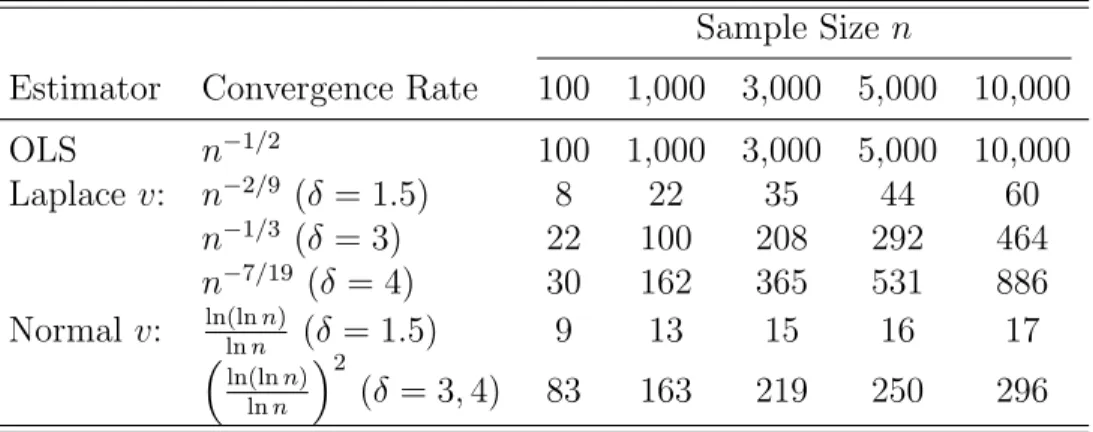
The proof is in the appendix. The proposed density estimator is semi-uniformly consis-tent. That is, ˆfu is uniformly consistent over a given class of Laplace distributions Ln. The optimal convergence rate for an ordinary-smooth target density is achieved in a minimax sense. It is similar to the conclusions in Fan (1991), even though in this exercise the variance of the noise distribution is unknown and the composed error needs to be estimated. The polynomial convergence rate plays a role in the following sense. After imposing the modified variance truncation device, which is the proposed best choice one can use for unknown vari-ance, and after deriving the optimal sequences for convergence (i.e., the order of the positive sequence {kn}n∈N), we still achieve a polynomial convergence rate which is consistent with the lower bound derived by Fan (1991).

At first glance the Theorem 1 is similar to Theorem 2 in Meister (2006), but there

are three major differences: (i) the upper bound of the noise v is not a known constant

but a consistently estimated (at √n rate) quantity (i.e., 1₄ln lnn versus 1₂V(ˆε)); (ii) the

chosen sequences are functions of the target density smoothness order, δ, which is due to

the characteristic function of the Laplace noise, leading to different convergence rates (or effective sample size as shown in Table 2); and (iii) we consider estimation in the regression

setting, which is more general than the pure deconvolution setting (β = 0), and yields

different convergence rates with Laplace noise. In Horrace and Parmeter (2011) this last difference was easily handled, given the slow convergence of the density estimator due to the assumption of super-smooth noise. It is more nuanced in the context of Laplace noise, given the polynomial rate of convergence. This has important implications if one were to

estimate the unknown conditional mean using nonparametric methods. We discuss this and other extensions of the Laplace deconvolution estimator in the next section.

4

Some Useful Extensions

We discuss two useful extensions to the Laplace deconvolution estimator which are likely to arise in applications: (i)C1 andδ are unknown in Assumption 3 and (ii) deploying

nonpara-metric regression to estimate the unknown conditional mean needed to subsequently recover ˆ

ε. It is rare in applications that researchers have information on the target density. This leads to uncertainty inC1 andδ, two parameters which are important in the implementation

of our estimator.13 _{Also, if we wish to follow the work of Fan, Li and Weersink (1996) and}

estimate the unknown regression function nonparametrically, then we must think carefully about the relative polynomial convergence rates of the deconvolution estimator and the non-parametric regression estimator. This is not a consideration with normal noise due to the logarithmic convergence rates it produces.

4.1

Selection of Unknown

C

and

δ

In the usual case that δ and C1 are unknown and, therefore, might be misspecified,14 we

could apply the following selection rule due to Meister (2006):

Selection rule 1. If C1 and δ are unknown, we specify one set of {C1, δ} and choose

wn=kn/lnkn.

13_{... and the estimator of Meister (2006) as well.}

14_{Actually, if one wants to assume the random noise is super-smooth with similarity indexs, the smoothness}

parameterδof target density can be estimated as well as thesby an adaptive procedure proposed by Butucea,

An alternative rule may be based on our procedure when δ and C1 are known. First, we

specify one set of parameters {C1, δ} to pin down the variance truncation device defined in

Section 2, and then by Lemmas 1 and 2 we determine the optimal choice for the sequence {kn}n∈N. The trade-off is a slower convergence rate of the estimated target density compared with that in the fully-known case due to lack of information about the target density. This implicitly requires a larger n to achieve a reliable estimate of the target density. This can be seen from following theorem.

Theorem 2. AssumeδandC1 are unknown. Under Assumption 1, 3, 4, and 5 set{b2n}n∈_N=

1 2V(ˆε) and wn = kn/lnkn with {kn}n∈N = {( n b2 n) 1 6+2δ} n∈N, if 1 < δ ≤ 1.5, or {kn}n∈N = {(_bn8 n) 1 3+4δ}

n∈N, if δ >1.5. For any g ∈ Ln, the proposed deconvolution kernel density estima-tor in equation (7) is bounded from above as following:

sup fu∈Fu Ef,g||fˆu−fu||2L2 ≤(n/lnn) −2δ−1 6+2δ if 1< δ ≤1.5 and sup fu∈Fu Ef,g||fˆu−fu||2L2 ≤(n/lnn) −2δ−1 3+4δ if δ >1.5

where δ is defined by Assumption 3.

The proof is similar to that of Theorem 1 in the appendix and is contained therein. The only difference between the bounds in Theorem 1 and in Theorem 2 is that the bounds are negative exponents of n in the former and of n/lnn in the latter, and this is the price one pays for not knowing the smoothness parameters of the target density. Based on the Theorem 2 and Table 1, we propose a rule-of-thumb adaptive procedure as follows:

0 and 1; δ is between 1 and 10.

Step 2: Treating this C1 and δ as “known,” selectkn =wn and apply the proposed

deconvolu-tion techniques to construct the estimated target density, ˆfknown(u), say.

Step 3: Now, with the same C1 and δ assume they are unknown and select wn = kn/lnkn.

Again, apply the proposed deconvolution estimator to construct the estimated target density as ˆfunknown(u), say.

Step 4: Compare thevector of values ˆfknown(u) and ˆfunknown(u) over a discretized support with

a Euclidean distance measure (e.g., ∆ = ||fˆknown(u)−fˆunknown(u)||2_{). Iterate Steps 1}

to 3 until ∆ is smaller than a pre-specified threshold, say 0.0001.

One caveat with this iterative approach is that ∆ may be quite large initially. The essential point is that more information about the underlying distribution is revealed after several trials with combinations of the smoothness parameters. This is similar in spirit to the adaptive procedure proposed by Butucea, Matias and Pouet (2008), but their targets are a “self-similarity index” and a smoothness parameter with super-smooth noise, and not a target density.

4.2

Nonparametric Estimation of the Conditional Mean

If one is unsure of the linear specification of the conditional mean, equation (1) can be generalized to the nonparametric case as follows:

where g(.) is unknown and x∈ Rq_{. Under certain regularity conditions,}15 _{a straightforward}

nonparametric kernel estimator for the unknown function g(x) is:

ˆ g(x) = Pn j=1YjK( Xj−x λ ) Pn j=1K( Xj−x λ )

where K(·) is the standard Gaussian kernel with bandwidth λ. Note that since the

con-vergence rate of the nonparametric estimator is a polynomial function of the number of covariates, this may impact application of the Laplace deconvolution estimator.

By Theorem 2.6 (with Condition 2.1) of Li and Racine (2007), the convergence rate of the estimated function is:

sup x∈S |ˆg(x)−g(x)|=O (lnn) 0.5 (nλ1· · ·λq)0.5 + q X s=1 λ2_s ! a.s.

Assuming each bandwidth (λs) has the same order of magnitude, the optimal choice of

λs that minimizes M SE[ˆg(x)] is λs ∼ n

− 1

4+q, and the resulting MSE is therefore of order

O(n−4+4q). Consequently, the estimated error, ˆε, is na consistent where a = 2

4+q. That is,

na_{(ˆε−ε) = O}

p(1) as n→ ∞.

Similarly, we can establish the convergence rate as follows:

Theorem 3. Under Assumptions 3-5, and Condition 2.1 in Li and Racine (2007) set

{b2 n}n∈N = 1 2V(ˆε) and wn =kn with {kn}n∈N ={( n b2 n) 2a 6+2δ}_n∈ N, if 1 < δ ≤1.5, or {kn}n∈N = {(_bn8 n) 2a 3+4δ}

n∈N, if δ >1.5. For any g ∈ Ln, the proposed deconvolution kernel density

tor in equation (7) is bounded from above as follows: sup fu∈Fu Ef,g||fˆu−fu||2L2 ≤n −2a₆₊₂(2δ−_δ1) if 1< δ ≤1.5 and sup fu∈Fu Ef,g||fˆu−fu||2L2 ≤n −2a(2δ−1) 3+4δ if δ >1.5

where a= ₄₊2_q and δ is defined by Assumption 3.

The proof is very similar to the proof of Theorem 1 in the appendix, and a sketch of the proof is contained therein.

5

Monte Carlo Simulations

We present a Monte Carlo study of the finite sample properties of the Laplace deconvolution estimator. For ease of comparison, we follow the sample designs of Meister (2006) and Hor-race and Parmeter (2011) except that we consider performance of the Laplace deconvolution with both Laplace noise (correctly specified) and normal noise (misspecified). We focus on sample sizes of n= 500, 1,000, and 3,000 with the linear model:

yj = 4 + 3xj+vj+uj, j = 1, . . . , n. (10)

The xjs are generated from a standard normal distribution. Random noise vj is generated

from either a standard Laplace (correctly specified) or normal (misspecified) distribution for a range of values of the variance to produce several signal-to-noise settings. The ujs are

density function is ˜L(x) = 1₄e−|x|(|x|+ 1).16 We fix the variance of u to 2. In this setting it is known that C1 = 1/4, δ= 4 andT = 1.17

Following Theorem 1, we choose b2_n = 1₂V(ˆε) where ˆε is the residual from the first-step

ordinary least squares (OLS) estimation, and kn = n

1 4δ+3(b2 n) −4 4δ+3 =n191 (b2 n) −4 19,

correspond-ingly asδ= 4 >1.5. To explore the impact of the relative ratio of the component variances, we consider different scenarios of the signal-to-noise ratio which is defined as the ratio of

V(u) and V(v): γ := σ2

u/σv2 ∈ {1/2,1,2}. We also apply our Laplace deconvolution esti-mator in the misspecified case where the errors are normally distributed. We compare the performance of our estimator under misspecification to the normal deconvolution estimator of Meister (2006) which is correctly specified. Even in this case, our estimator performs fairly well. We also explore the finite sample performance of our proposed rule-of-thumb adaptive procedure when the smoothness parameters of the target density are unknown.

The performance of our estimator is assessed through the root mean integrated square error (RMISE): RM ISE( ˆfu) = v u u t 1 R R X l=1 1 M M X i=1 ( ˆfl(ui)−f(ui))2 (11)

where R is the number of replications andM = 256 is the number of evaluation points over

u∈(−5,5), which is fixed across the R replications.

5.1

Laplace Deconvolution with Laplace Errors

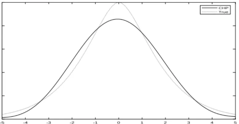
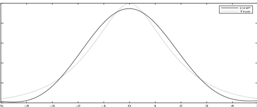
First, we consider the case that the random noise vj is correctly specified (i.e., vj is drawn

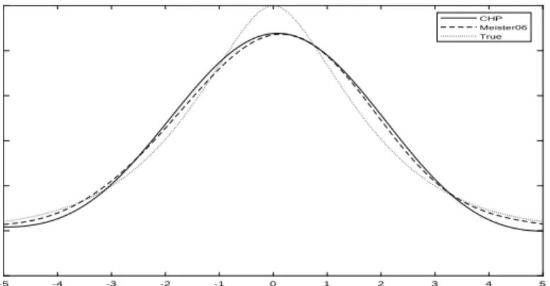
from a Laplace distribution with variance 1). Figures 1-3 show the results for a single

random draw (R = 1) across various sample sizes {500, 1,000, 3,000} and compare the

proposed estimator (CHP) to the true unknown density (T rue). The graphical fit of the

16_{This follows from the setting in Meister (2006).}

17_{We are not concerned withC}

proposed estimator is quite good with only 500 observations (Figure 1). Most of the bias

comes from estimation around the mode.18 As the sample size increases, the RMISE of the

proposed estimator (CHP) decreases from 0.0148 (Figure 1) to 0.0142 (Figure 2) and to

0.0125 (Figure 3).

Figures 4-6 show the results for a single draw (R = 1) and fixed sample size n =1,000

but varying the signal-to-noise ratio σ2

u/σ2v = 2/1,2/2,2/4. The proposed estimator (CHP)

works very well when σ2

u/σv2 = 2/1 with 1,000 observations. As the signal-to-noise ratio

decreases, the RIMSE of proposed estimator (CHP) increases from 0.0136 (Figure 4) to

0.0142 (Figure 5) and to 0.0180 (Figure 6). Even for the noisiest case (Figure 6) with

σ_u2/σ2_v = 2/4, the fit is very good except in an interval around the mode.

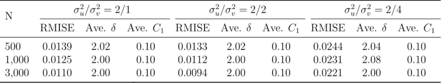
Table 3 contains detailed results from R = 500 simulations with varying sample sizes

{500, 1,000, 3,000} and signal-to-noise ratios {1/2, 1, 2}. For each signal-to-noise setting (each column), the RMISE decreases monotonically as the sample size increases from 500

to 3,000 (down the rows), demonstrating the consistency of the proposed estimator (CHP).

Unexpectedly, the RMISE is not increasing as the signal-to-noise ratio increases across the columns. This is an atypical finding that is due to the variance truncation device: when the variance of the random noise is relatively small, the estimated variance parameter ˆb2_nis more

likely to be closer to zero which dilutes the ability of the deconvolution estimator to recover the target density. Alternatively, when the variance of the random noise is relatively large, the estimated variance is no longer near zero, but the performance of the deconvolution estimator deteriorates as there is little information in the target density taken from the compound errors. This is a limitation of the variance truncation device.

18_{Estimation of a density around the mode is difficult due to the derivative at the mode being zero}

5.2

Laplace Deconvolution with Misspecified Noise

To understand the impact of misspecification of the noise distribution, we consider the per-formance of the proposed estimator when the true noise is distributed normal. We compare

the performance of our proposed estimator (CHP) with that of Meister (2006).

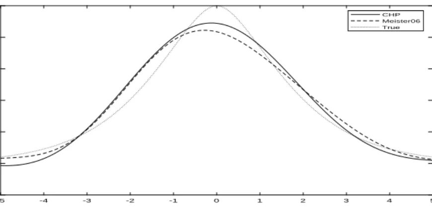
As a first pass on the empirical performance, Figures 7-9 show the results for the case with fixed σ_u2/σ2_v = 2/2 for a single draw (R= 1) across various sample sizes. The proposed

estimator (CHP) shows decent performance even with sample size of n = 500 (Figure 7).

The figure contains plots of the proposed estimator (CHP), the estimator of Meister (2006)

(M eister06), and the true normal density (T rue). As the sample size increases, the RMISE

of the proposed estimator (CHP) changes from 0.0151 (Figure 7) to 0.0156 (Figure 8) to

0.0137 (Figure 9). Our estimator (CHP) performs as well as Meister’s when the sample

size is large (n= 3,000). An intuitive explanation is that the proposed estimator converges faster than Meister’s estimator (even under misspecification).

Figures 10-12 show the results for R = 1 and fixed sample size n = 1,000 across the

various signal-to-noise ratios. The proposed estimator (CHP) performs quite well in the

least noisy case even though the error distribution is misspecified. As the signal-to-noise ratio decreases, the RIMSE of the proposed estimator increases from 0.0155 (Figure 10) to 0.0156 (Figure 11) and to 0.0191 (Figure 12) whereas the RMISE of Meister’s estimator increases from 0.0120 (Figure 10) to 0.0172 (Figure 11) to 0.0260 (Figure 12). When the signal-to-noise ratio decreases from 1 to 0.5 (Figures 11 and 12, respectively) the misspecified estimator even outperforms Meister’s estimator.

Table 4 presents the results ofR = 500 replications across various sample sizes and signal-to-noise ratios under misspecification. Though misspecified, the RMISE of the proposed estimator decreases monotonically as the sample size increases (down each column) for each signal-to-noise ratio setting, and it is comparable to that of Meister’s correctly specified

estimator. In the most noisy setting, σ_u2/σ_v2 = 2/4, the proposed estimator outperforms

Meister’s estimator across all sample sizes. This may be due to the faster convergence rate of the proposed estimator coupled with the fact that the characteristic functions of the normal and the Laplace are quite similar.19 _{Fixing the sample size (within each row), both}

RMISEs increase when the signal-to-noise ratio decreases as the information that can be recovered is reduced. Overall, the proposed estimator is robust to misspecification of the error distribution and its convergence rate is faster than that of Meister’s estimator.

5.3

Deconvolution With Unknown Smoothness Parameters

To verify the feasibility and performance of the proposed rule-of-thumb adaptive procedure for unknown smoothness parameters of section 4.1, a set of simulations are performed. We employ the same simulation design. Specifically, the true target density is still a

twice-convolved Laplace with true smoothness parameters ofC1 = 1/4 andδ= 4. We search on a

two-dimension grid of C1 ∈ {0.1,0.25,0.40,0.55,0.70,0.85} and δ ∈ {2,4,6,8} to minimize

the Euclidean distance of the two estimated densities: the estimated density assuming the

chosen C1 and δ are known and the estimated density assuming these parameters are

un-known. We restrict the range ofu to be (−5,5) and evaluate over 128 evenly spaced points within this range.

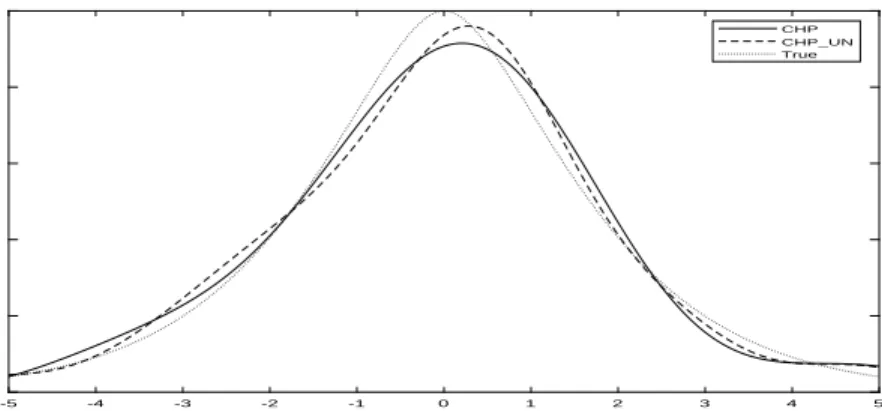
Figure 13 shows the estimated densities (labeled CHP for the estimate with known

smoothness parameters and CHPU N for the estimate with unknown parameter) and the

true density (labeled T rue) for one simulation (R = 1) with sample size n = 1,000 and

signal-to-noise ratio equal to 1. The chosen smoothness parameters are: C1 = 0.1 andδ = 2.

Even though the chosen smoothness parameters are misspecified (not exactly equal to the their true valuesC1 = 1/4 andδ= 4), the overall fit of the density with estimated parameters

is quite good (CHPU N) and appears to be better than the fit assuming the true values of

the parameters, particularly around the mode.20

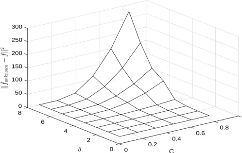
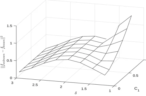
A more comprehensive analysis is conducted in Figures 14-16. Figure 14 shows the

Euclidean distance of the estimated densities: ∆ = ||fˆknown −fˆunknown||2, as a function of

the smoothness parameters for a single draw (R = 1). Figures 15 and 16 show the Euclidean

distance between the true density and the estimated density taking the chosen C1 and δ

as known, ||fˆknown −ftrue||2, and unknown, ||fˆunknown − ftrue||2, respectively. A straight comparison of the three figures indicates that the convergence pattern is almost identical which means that minimizing the Euclidean distance of the estimated densities (Figure 14) is almost equivalent to minimizing the Euclidean distance of the estimated density and the true underlying density (Figures 15 and 16). Obviously, the Euclidean distance is smaller for values around the true smoothness parameters (C1 = 1/4 and δ= 4) in this context.

Although it is a useful tool, our adaptive procedure comes with two caveats. First, our Laplace deconvolution estimator assumes that the noise distribution is Laplace. If this assumption is violated, the adaptive procedure may not perform as well as we see here. Second, the Euclidean distance between the true density and the estimated density achieves small values in a range of smooth parameters rather than at one specific point in Figure 14. It indicates that the proposed rule-of-thumb adaptive procedure is informative for providing a small range of the smoothness parameters rather than one optimal point.

To calculate the RMISE when the smoothness parameters are unknown, we replicate the

above simulations for R = 100 with various sample sizes and signal-to-noise ratios.21 _The

results are presented in Table 5.22 _{Similar to Table 3, the convergence pattern still holds}

20_{The reader is reminded that the fit of the estimated densities, whether with or without known smoothness}

parameters, is a function of the Euclidean distance evaluated over the 128 points in their support. Therefore, the relative fit of the densities with known and unknown parameters will vary over this support. That is, we should not expect the density with known parameters to always have better fit than the estimated density with unknown parameters. This is reflected in Figure 13

21_{We reduce the replication size from 500 to save computation time.}

22_{We report the RMISE of ˆf}

when the sample size increases with fixed signal-to-noise ratios. That is, reading down the columns, RMISE is decreasing in the sample size. As we read across RMISE columns within a row, the RMISE is decreasing slightly and then increasing. We also report the chosen

smoothness parameters, δ and C1, based on minimizing the Euclidean distance in Table 5.

They vary slightly around 2 and 0.1, respectively. They are not always accurate (compared to the true values) but still render reasonably good estimates of the target density.

6

Applications

In this section two applications demonstrate the utility of the proposed method. We consider the parametric Laplace stochastic frontier model (Horrace and Parmeter, 2018), a regression-based application of the method, and a second application where the outcome of interest, daily saturated fat intake, is contaminated with measurement error (which we assume to

be Laplace) and β = 0 in equation (1). In the first application we assume the smoothness

parameters are known; in the second we use our adaptive rule-of-thumb to select them.

6.1

Stochastic Frontier Analysis

A typical parametric stochastic frontier model is equation (1), but restricting u < 0 (for a production frontier) or u > 0 (for a cost frontier). Given distributional assumptions on in-efficiency, u (e.g., exponential or half-normal) and noise, v (e.g., normal or Laplace), β may be consistently estimated and used to calculate the conditional distribution of firm-level inefficiency, which is typically characterized by the empirical distribution of u conditional

on ε (e.g., Jondrow et al. 1982). Much of the existing literature assumes normality of v

ticulated by Kneip, Simar, and Van Keilegom (2015, p.380) who note that “. . . there does usually not exist any information justifying particular distributional assumptions on (ineffi-ciency).” Additionally, Tsionas (2017, p.1169) suggests that a model constructed to provide microfoundations for the presence of inefficiency “. . . does not make a prediction about the distribution.” These statements underlie the importance of seeking alternative estimation approaches to recover important features of the stochastic frontier model; those approaches which eschew restrictive parametric assumptions are likely to curry favor among practitioners and regulators alike.

There is also no reason to favor normally distributed errors in the stochastic frontier model (Horrace and Parmeter, 2018). As such we apply our Laplace deconvolution estimator to estimate the distribution of inefficiency from a cost frontier for US banks. The data come from Feng and Serletis (2009) and are obtained from the Reports of Income and Condition (Call Reports).23

The data are a sample of US banks covering the period from 1998 to 2005 (inclusive). After deleting banks with negative or zero input prices, we are left with a balanced panel of 6,010 banks observed annually over the 8-year period. A more detailed description of the data may be found in Feng and Serletis (2009). For our purposes we ignore the panel structure of the data and choose the most recent year data, 2005, for our example. The goal of this exercise is to estimate the marginal distribution of u and compare it with the typical half-normal distribution which informs practical choice of parametric assumption on

u, which , in turn, informs estimation of E(u|ε).24

The data contain information on three output quantities and three input prices. The three outputs are consumer loans, Y1; non-consumer loans, Y2, which consists of industrial

23_{The data are publicly available on the Journal of Applied Econometrics data archive website}

http://qed.econ.queensu.ca/jae/2009-v24.1/feng-serletis/.

24_{Once ˆf}

u is obtained, one can estimate the efficiency score using numerical integration on a grid of ˆε. To

and commercial loans and real estate loans; and securities,Y3, including all non-loan financial

and physical assets minus the sum of consumer loans, non-consumer loans, securities and equity. All outputs are deflated by the Consumer Price Index (CPI) to the base year of 1988. The three input prices are: the wage rate for the labor, P1; the interest rate for borrowed

funds, P2 and the prices of physical capital, P3. The total cost, C, is the sum of three

corresponding input costs: total salaries and benefits, expenses on premises and equipment, and total interest expenses. Our specification of output and input prices is the same as (or very similar to) what is typical in the literature (see, for example, Feng and Serletis, 2009; Kumbhakar and Tsionas, 2005.) The cost frontier model is

cj =α+x0jβ+uj+vj j = 1, . . . , n, (12)

where cj = lnCj; xj = lnXj with Xj including the three output quantities and three input

prices: Y1, Y2, Y3, P1, P2, P3; and uj >0 is firm-specific inefficiency.

We estimate the distribution of cost inefficiency in three ways. First, we estimate a fully parametric model, assuming v is distributed N(0, σ_v2) and u is distributed |N(0, σ_u2)|.

Our maximum likelihood estimates of the distributional parameters are ˆσu = 1.294 and

ˆ

σv = 0.989, implying E(u) = ˆσu

p

2/π = 1.033. Then, our estimate of the density of u is |N(0,1.2942_{)|, which is shown as the dotted line (SF A) in Figure 18. Second, we estimate}

equation (12) by OLS. Figure 17 shows a histogram of the OLS residuals, ˆεj. The asymmetry

of the distribution (skew equals 1.550) suggests non-zero cost inefficiency.25 _{Selecting δ= 3}

andC1 = 1 and using Theorem 1, the deconvolution estimator yields an estimate ofσ2v equal

to 0.0403.26 A plot of the density estimate, ˆfu(u), is shown as the dashed line (CHP) in

25_{It is interesting to note that with a skew of 1.55, this provides evidence against use of the half-normal}

distribution.

Figure 18. Third, using the procedure of Hall and Simar (2002) with a bandwidth of 0.3052, we detect a jump discontinuity point in ˆfu(u) at u = −0.355 which implies an estimate of

ˆ

E(u) = 0.355. Then using the boundary kernel proposed by Zhang and Karunamuni (2000),

with an estimated error variance of 0.0403 (as before), the boundary bias corrected density estimate is shown as the solid line (CHP E(u) bc) in Figure 18.27

Figure 18 shows all three density estimators for US bank inefficiency in 2005. Notice that even without a boundary correction, the deconvolution estimator (CHP) has a thinner right tail than the estimated half normal density (SFA). With boundary correction in place, the

deconvolution estimator (CHP E(u) bc) implies that US banks in 2005 have a much smaller

average inefficiency than parametric SFA would have predicted. This corresponds to the fact that in 1998 there are 10,139 banks in the US and this number declined to 8,390 in 2005 due to industry consolidation (Feng and Serletis, 2009).

Finally, there are at least two reasons to employ the proposed estimator: 1) the proposed method provides a robustness check for the distributional assumptions made in a parametric stochastic frontier model and 2) the skewness of the OLS residuals is greater than one, which invalidates the choice of the half-normal assumption for the distribution of u (which has maximal skewness of 1 by definition).

6.2

Daily Saturated Fat Intake With Measurement Errors

The data come from Wave III (1988-1994) of the National Health and Nutrition Examination Survey, abbreviated NHANES III. Our interest is the survey response to daily saturated fat intake of 3,551 women between the ages of 25 and 50. This data set is ideally suited to our Laplace deconvolution estimator as it is well established that saturated fat consumption is recorded with measurement errors. In fact, previous analysis of the NHANES Wave I

(1971-75) and Wave II (1976-1980) data suggest that more than 50% of the variability in the observed data may be due to measurement errors. See Stefanski and Carroll (1990), Carroll, Ruppert and Stefanski (2006) and Delaigle and Gijbels (2004).

The data were originally recorded to explore the relationship between breast cancer and dietary fat intake, see Jones et al. (1987). Stefanski and Carroll (1990) were the first to consider nonparametric deconvolution techniques to estimate the underlying true density of saturated fat intake, using NHANES I. Subsequently, Carroll, Ruppert and Stefanski (2006), Delaigle and Gijbels (2004) and others applied deconvolution estimators to NHANES II. In each of these applications a normal error distribution was assumed. To the best of our knowledge we are the first to apply deconvolution techniques to NHANES III (and certainly the first to apply Laplace deconvolution to any of these data). Here, saturated fat (f at) is measured in milligrams per day, and we apply the same data transformation as Delaigle and Gijbels (2004): log(f at+ 5).

To these data we implement a) the proposed estimator with Laplace errors (CHP), b) the estimator with normal errors due to Meister (2006) (M eister), and c) an error free estimator

(ErrorF ree), based on pure kernel density estimation of the observed data assuming there

is no measurement error.28

First, we apply the proposed rule-of-thumb adaptive procedure to get a preliminary estimate of the smoothness parameters since they are unknown. Specifically, we search for the minimum of the Euclidean distance between the density estimator with unknown smoothness parameters and density estimator with known smoothness parameter, ∆, over a grid of δ ∈ {1.25,1.5,1.75,2,2.25,2.5,2.75,3} and C1 ∈ {0.1,0.25,0.40,0.55,0.70,0.85,1}.29

Figure 19 shows the surface of the Euclidean distance as a function of the smoothness

parameters over the grid. The ∆ increases as C1 rises from 0 to 1 except when δ is around

28_{We use the package “ksdensity” in Matlab for theErrorF reecase.}

2. It seems that δ = 1.5 and δ = 3 yield the minimum distance. It turns out that when

δ= 3, the estimated density decreases very quickly and goes below zero and becomes volatile when log(f at+ 5) <2 or log(f at+ 5)>4.5. Therefore, we consider the δ= 1.5 case to be optimal. Specifically, we chooseC1 = 1 andδ= 1.5 as our baseline model. We then consider

alternative specifications of the smoothness parameters as a robustness check.

Figure 20 presents the final results of the analysis. The estimated error variance is 0.065 based on theCHP estimator and 0.525 based on theM eisterestimator in the baseline model.

The M eister error variance estimate is exceedingly large compared to the variance of the

observed (convoluted) data, 0.236.30 The CHP error variance estimate is more reasonable

in the sense of being less than the total observed variance, and its corresponding signal-to-noise ratio is 0.275. This is consistent with the finding in the existing literature that about 30-50% of the variability of observed data is due to measurement error. The tail behaviors

in Figure 20 shows that the M eister estimator assigns more variance to the error variance

than expected and it decreases to zero very quickly. TheCHP estimator extracts the target

density information based on the smoothness assumptions, which gives a reasonable variance estimate and tends to have longer tails.31

The CHP density estimator based on the NHANES III data is quite similar to that of

Delaigle and Gijbels (2004), despite the fact that they used the NHANES II data, assumed the error to be normal, along with differing identification assumptions. They experiment with different “known” values of the signal-to-noise ratio, while we have to select the smoothness parameters. The minor difference is that our estimated tails are slightly thicker than theirs, however the means of the estimated densities are nearly identical.

As a robustness check, different combinations for the values of δ and C1 are considered

for the CHP estimator: C1 = 1 and δ = 1.5; C1 = 1 and δ = 2; C1 = 0.6 and δ = 1.5;

30_{It seems to violate the independence assumption between the target variable and the measurement error.}

31_{Under Assumption 1, i.e.,uandvare independent, the variance ofY should be the sum of the variances}

C1 = 0.6 and δ = 2 in Figure 21. The baseline (C1 = 1, δ = 1.5) is in the upper-left

panel of the figure. As we move to different panels in the figures we change the values

of the smoothness parameters, so the CHP estimator is changing across panels, while the

ErrorF ree estimator is fixed. For C1 = 0.6, δ = 1.5 (lower-left panel), the estimated error

variance of CHP is 0.019 which is less than the baseline model, and it has less fat tails.

For C1 = 1, δ = 2 (upper-right panel), the estimated error variance of CHP is 0 which

makes it nearly coincide with the ErrorF ree case.32 _{This means that it is more difficult}

for information on the measurement error to be be disentangled under these smoothness assumptions. We can also varyC1 to recover certain information concerning the noise or the

error term. For instance, C1 = 0.6, δ = 2 (lower-right panel), the estimated error variance

of CHP is still 0 which renders an identical deconvolution density estimate. It seems that

the variability of δ dominates that of C1. This is intuitive as τ → ∞, the effect of C1 is

ignorable in Assumption 3.

7

Conclusion

This paper proposes a semiparametric estimator for a cross-sectional error component model. Instead of focusing on the estimation of the model parameters with the typical assumption of normality, we are interested in the density of the target error component. To estimate the target density without fully known random noise, we modify the variance truncation device proposed by Meister (2006) and extend the methodology to the framework of an error component model with a Laplace noise term with unknown variance.

The density deconvolution estimator with Laplace noise has at least two attractive char-acteristics for applied researchers: 1) it possesses a faster convergence rate than that of

normal distributed noise (i.e.,O(nc) versusO((lnn)c)) and 2) it is robust to misspecification

of the true underlying noise distribution. A third (potential) feature that practitioners may find appealing is the Laplace noise generates different insights than normal noise: for ex-ample, the LAD estimator rather than OLS, the Laplace stochastic frontier model (Horrace and Parmeter, 2018) and the L-SIMEX estimator (Koul and Song, 2014).

For future research, it may be useful to extend the model to panel data and use it to estimate both the target and noise distributions nonparametrically. For example, with a nonparametric production or cost function this would imply a fully nonparametric stochastic frontier model. Jirak, Meister and Reiss (2014) studied adaptive function estimation in

nonparametric regression with one-sided errors. Another interesting strand in this area

is to investigate the distribution of unobserved heterogeneity with proposed deconvolution techniques. Recently, Evdokimov (2010) takes an initial step to explore that in a panel data model and Ju, Gan and Li (2019) apply it to a labor data set.

References

[1] Butucea, C. and C. Matias, Minimax Estimation of the Noise Level and of the Decon-volution Density in a Semiparametric ConDecon-volution Model. Bernoulli. 2005, pp. 309-340. [2] Butucea, C., C. Matias, and C. Pouet, Adaptivity in Convolution Models with Partially

Known Noise Distribution. Electronic Journal of Statistics. 2008, pp. 897-915.

[3] Cao, C. D. Linear Regression with Laplace Measurement Errors. Master Thesis. De-partment of Statistic, Kansas State University.

[4] Carroll, R.J., D. Ruppert, L. A. Stefanski, and C. M., Crainiceanu. Measurement Error in Nonlinear Models: A Modern Perspective, volume 2nd Ed. CRC Press, 2006.

[5] Delaigle, A. and I. Gijbels. Practical bandwidth selection in deconvolution kernel density estimation. Computational Statistics & Data Analysis. 2004. 45 (2) pp. 249-267. [6] Evdokimov, K., Identification and Estimation of a Nonparametric Panel Data Model

with Unobserved Heterogeneity. 2010, Working paper version.

[7] Fan, J., On the Optimal Rates of Convergence for Nonparametric Deconvolution Prob-lems. Annals of Statistics. 1991, pp. 1257-1272.

[8] Feng, G. H., and A. Serletis, Efficiency and Productivity of the US Banking Industry,1998-2005: Evidence from the Fourier Cost Function Satisfying Global Regu-larity Conditions. Journal of Applied Econometrics. 2009, 24, pp.105-138.

[9] Greene, W. H., A gamma-distributed stochastic frontier model, Journal of Economet-rics. 1990, 46(1-2), 141-164.

[11] Henderson, D. J. and C. F. Parmeter. Applied Nonparametric Econometrics. 2015, Cambridge University Press.

[12] Hesse, C. H., Data-driven Deconvolution. Nonparametric Statistics. 1999, 10, pp. 343-373.

[13] Horowitz, J. L., and M. Markatou, Semiparametric Estimation of Regression Models for Panel Data. Review of Economics Studies. 1996, 63, pp. 145-168.

[14] Horrace, W. C., Moments of the Truncated Normal Distribution. Journal of Productivity Analysis. 2015, 43, pp. 133-138.

[15] Horrace, W. C., and C.F. Parmeter, Semiparametric Deconvolution with Unknown Er-ror Variance. Journal of Productivity Analysis. 2011, 35, pp. 129-141.

[16] Horrace, W. C., and C.F. Parmeter, A Laplace Stochastic Frontier Model. Econometric Reviews. 2018, 37, pp. 260-280.

[17] Jirak, M., A. Meister, and M. Reiss. Adaptive function estimation in nonparametric regression with one-sided errors. Annals of Statistics. 2014, 42(5), pp. 1970-2002. [18] Jondrow, J., C. K. Lovell, I. S. Materov, and P. Schmidt, On the Estimation of Technical

Inefficiency in the Stochastic Frontier Model. Journal of Econometrics. 1982, 19, pp. 233-238.

[19] Jones, D.Y., et al. Dietary fat and breast cancer in the National Health and Nutrition Examination Survey I Epidemiologic Follow-up Study. Journal of the National Cancer Institute. 1987. 79(3), pp. 465-71.

[20] Johannes, J., Deconvolution with Unknown Error Distribution. Annals of Statistics. 2009, 37, pp. 2301-2323.

[21] Ju, G., L. Gan, and Q. Li. Nonparametric panel estimation of labor supply. Journal of Business & Economic Statistics. 2019, 37(2), pp. 260-274.

[22] Koul, H.L., and W.X. Song. Simulation Extrapolation Estimation in Parametric Models with Laplace Measurement Error. Electronic Journal of Statistics. 2014, 8, pp. 1973-1995.

[23] Kneip, A., L. Simar, and I. Van Keilegom. Frontier estimation in the presence of mea-surement error with unknown variance. Journal of Econometrics. 2015, 184(2), pp. 379-393.

[24] Kumbhakar, S. C. and E. G. Tsionas, Measuring Technical and Allocative Inefficiency in the Translog Cost System: A Bayesian Approach. Journal of Econometrics. 2005, 126, pp. 355-384.

[25] Kumbhakar S. C., B.U. Park, L. Simar, E.G. Tsionas. Nonparametric stochastic fron-tiers: a local likelihood approach. Journal of Econometrics. 2007, 137(1), pp. 1-27. [26] Kumbhakar, S.C., C.F. Parmeter, and V. Zelenyuk. Stochastic Frontier Analysis:

Foun-dations and Advances. CEPA Working Papers Series WP022018, School of Economics, University of Queensland, Australia.

[27] Li, Q. and J.S. Racine. Nonparametric Econometrics: Theory and Practice. 2007, Princeton University Press.

[28] Meeusen, W. and J. van den Broeck. Efficiency estimation from Cobb-Douglas produc-tion funcproduc-tions with composed error, Internaproduc-tional Economic Review. 1977, 18(2), pp. 435-444.

De-[30] Meister, A., Density Estimation with Normal Measurement Error with Unknown Vari-ance. Statistica Sinica. 2006, 16, pp. 195-211.

[31] Meister, A., Deconvolution Problems in Nonparametric Statistics. 2009. Lecture Notes in Statistics 193. Springer, Berlin

[32] Neumann, M. H., On the effect of Estimating the Error Density in Nonparametric Deconvolution. Nonparametric Statistics. 1997, 7, pp. 307-330.

[33] Nguyen, N. B., Estimation of technical efficiency in stochastic frontier analysis. 2010, PhD thesis, Bowling Green State University.

[34] Parmeter, C. F., H. J. Wang, and S. C. Kumbhakar. Nonparametric estimation of the determinants of inefficiency. Journal of Productivity Analysis. 2017, 47, pp. 205-221. [35] Parzen, E., On Estimation of A Probability Density Function and Mode. Annals of

Math Statistics. 1962, 35, pp. 1065-1076.

[36] Ritter, C. and L. Simar. Pitfalls of normal-gamma stochastic frontier models. Journal of Productivity Analysis. 1997, 8(2), pp. 167-182.

[37] Simar, L., I. van Keilegom, and V. Zelenyuk. Nonparametric least squares methods for stochastic frontier models. Journal of Productivity Analysis. 2017, 47, pp. 189-204. [38] Song, W.X., J.H. Shi, and C.X. Zhang. Linear errors-in-variables regression and

Tweedie’s formula. 2016. Working paper

[39] Stevenson, R. Likelihood functions for generalized stochastic frontier estimation. Journal of Econometrics. 1980, 13(1), pp. 58-66.

[40] Tran, K. C. and E. G. Tsionas. Local GMM estimation of semiparametric panel data with smooth coefficient models. Econometric Reviews. 2010, 29, pp. 39-61.

[41] Wang, W. S., C. Amsler, and P. Schmidt, Goodness of fit tests in stochastic frontier models. Journal of Productivity Analysis. 2011, 35, pp. 95-118.

[42] Wang, W. S. and P. Schmidt, On the Distribution of Estimated Technical Efficiency in Stochastic Frontier Models. Journal of Econometrics. 2009, 148, pp. 36-45.

[43] Wang, X. F. and D. Ye, The Effects of Error Magnitude and Bandwidth Selection for Deconvolution with Unknown Error Distribution. Journal of Nonparametric Statistics. 2012, 24, pp. 153-167.

[44] Zhang, S. and R. J. Karunramuni, Boundary Bias correction for Nonparametric Decon-volution. Annals of Institute Statistic Mathematics. 2000, 52, pp. 612-629.

A

General Appendix

Definition: ε is ordinary-smooth of orderδ (Fan 1991): characteristic function φε(t) satisfies

d0|t|−δ ≤ |φε(t)| ≤ d1|t|−δ as t → ∞.This is literally the same with the Assumption 3, just

replacing φε(t) with hε(τ).

A generalized result of Parseval’s identity (or the Plancherel theorem) asserts that the integral of the square of the Fourier transform of a function is equal to the integral of the square of the function itself.

In one-dimension, for f ∈L2(R), Z ∞ −∞ |fˆ(z)|2_{dz =} Z ∞ −∞ |f(τ)|2_dτ

where ˆf(z) = R_−∞∞ e−iτ z_{f(τ)dτ is the Fourier transform of the function f(τ).}

B

Proof of Lemma 1

There is a N so that wn > T holds for all n ≥ N. Hence the upper and lower bound of

the Fourier Transform can be used. Similar to Lemma 1 in Meister(2006), using Parseval’s identity and Fubini’s theorem, we have:

sup g∈Ln sup f∈Fu Ef,g||fˆu −fu||2L2 = 2π) −1 sup g∈Ln sup f∈Fu Z wn −wn Ef,g|e−iτ z ˆhε(1 + ˆˆ b2nτ 2 )−hu(τ)|2dτ+ Z |τ|>wn |e−iτ zhu(τ)|2dτ

P arseval = (2π)−1 sup g∈Ln sup f∈Fu Z wn −wn Ef,g|ˆhˆε(1 + ˆb2nτ 2 )−hu(τ)|2dτ + Z |τ|>wn |hu(τ)|2dτ ≤(2π)−1 sup g∈Ln sup f∈Fu 2 Z ∞ wn |hu(τ)|2dτ + sup g∈Ln sup f∈Fu 2 Z wn −wn Ef,g|(1 + ˆb2nτ 2_)(ˆh ˆ ε(τ)−hε(τ))|2dτ+ sup g∈Ln sup f∈Fu 2 Z wn −wn Ef,g|hε(τ)/ 1 (1 + ˆb2 nτ2) −hu(τ)|2dτ

The first term, which we call B, represents the bias which does not depend on the fact

that the convoluted errors are estimated and can be bounded as in Lemma 1 of Meister (2006). The second term can be split into two pieces, V1 and V2, where V1 is similar to

V in Lemma 1 of Meister (2006) while V2 is an additional component of the variance due

to estimating the composed errors. Our third term, which we call E, can be found almost

as that in Lemma 1 of Meister (2006) but the form of the bound is more complicated due to the fact that the empirical characteristic function used to construct the variance of the Laplace noise is constructed with ˆε instead of ε. The nonparametric regression in the first step impacts the convergence rate through the estimation of ˆε.

The following proof is similar to Meister (2006) and Horrace and Parmeter (2011) except now we deal with Laplace noise and a nonparametric first-step regression estimator rather than just normal noise for the linear (stochastic frontier) model. There are three steps to the proof.

(1) B ≤const×w1−2δ

(2) By assumption 5, ˆ hε(ˆ τ) = 1 n n X j=1 eiτεˆj = 1 n n X j=1 eiτ εj_{(1 +Op(τ n}−a₎₎ = (1 +Op(τ n−a))|ˆhε(τ)|

where a = ₄₊2_q for the nonparametric first-step regression and a = 0.5 for parametric

first-step regression, e.g, translog in the stochastic frontier model. We focus on the parametric setting hereafter for the main formulas and lay out the details of the differences when first-step nonparametric regression is implemented.33 _So

ˆ hεˆ(τ) =| 1 n n X j=1 eiτεˆj_|=|1 n n X j=1 eiτ εj_{(1 +O} p(τ n−1/2))|= (1 +Op(τ n−1/2))|hˆε(τ)| LetA(ˆhε) = Rwn −wnEf,g| ˆ hε(τ)−hε(τ)|2dτ = Rwn −wnEf,g| 1 n Pn j=1e iτ εj−_E(eiτ ε₎|2_{dτ =O} p(n−1wn), sup g∈Ln sup f∈Fu 2 Z wn −wn Ef,g(1+ˆb2nτ2)2|ˆhεˆ(τ)−hε(τ)|2dτ ≤4(1+ˆb2nwn2)2 sup g∈Ln sup f∈Fu Z wn −wn [Ef,g|ˆhεˆ(τ)−ˆhε(τ)|2+ Ef,g|ˆhε(τ)−hε(τ)|2]dτ = 4(1 + ˆb2_nw2_n)2 sup g∈Ln sup f∈Fu Z wn −wn Ef,g|ˆhˆε(τ)−hˆε(τ)|2dτ+ 4(1 + ˆb2nw 2 n) 2_A(ˆh ε) ≤4(1 +b2_nw_n2)2 sup g∈Ln sup f∈Fu Z wn −wn τ2Ef,g(n−1 n X j=1 |εˆj −εj|)2dτ + 4(1 +b2nw 2 n) 2_A(ˆh ε) = V1+V2

where V1 ≤const×(n−1wn3)(1 +b2nwn2)2 and V2 ≤const×(n−1wn)(1 +b2nw2n)2 .

(3) Similar to Lemma 1 in Meister (2006), for the last term we can derive:

E = sup g∈Ln sup f∈Fu 2 Z wn −wn Ef,g| hu(τ)(1 + ˆb2nτ2) 1 +b2_τ2 −hu(τ)| 2_dτ τ=swn = sup g∈Ln sup f∈Fu 2 Z 1 −1 Ef,g| s2w2_n(ˆb2_n−b2) 1 +b2_s2_w2 n |2_|h u(swn)|2wnds, where Ef,g| s2w_n2(ˆb2_n−b2) 1 +b2_s2_w2 n |2 _=E f,g| s2w_n2(ˆb2_n−b2) 1 +b2_s2_w2 n |2_χ(|ˆb2 n−b2| ≤dn) +Ef,g| s2w2_n(ˆb2_n−b2) 1 +b2_s2_w2 n |2_χ(|ˆb2 n−b2|> dn) ≤ | s 2_w2 ndn 1 +s2_w2 nb2 |2_+| s 2_w2 nb2n 1 +b2_w2 ns2 |2_{P r(|ˆb}2 n−b2|> dn) ≤(s 2_w2 ndn s2_w2 nb2 )2+ (s 2_w2 nb2n s2_b2_w2 n )2P r(|ˆb2_n−b2|> dn) ≤(dn b2) 2_{+ (}b 2 n b2) 2_{P r(|ˆb}2