Statistical Inference for Discrete-Valued Stochastic Processes

(1)

Inaugural - Dissertation

zur

Erlangung der Doktorw¨

urde

der

Naturwissenschaftlich-Mathematischen Gesamtfakult¨

at

der

Ruprecht-Karls-Universit¨

at

Heidelberg

vorgelegt von

Diplom-Mathematiker Sebastian Schweer

aus Freiburg im Breisgau

(2)

(3)

Statistical Inference for Discrete-Valued

Stochastic Processes

(4)

(5)

Acknowledgements

I would like to thank Prof. Dr. Rainer Dahlhaus, my supervisor, for his great support during my studies at the University of Heidelberg. I have had the honor to be his student ever since my undergraduate years and I am grateful for everything he taught me during these years.

Dr. Cornelia Wichelhaus has contributed a lot to my education, and without her constant encouragement I would have never achieved as much as I did. I would like to thank her for all the time we spent working together, starting with my diploma thesis and culminating in our joint contribution discussed in this thesis.

I am grateful to have made the acquaintance of Prof. Dr. Christian Weiß during my PhD research. Discussing problems and new approaches with him has not only been enlightening but also very enjoyable, and I owe him special gratitude for his willingness to share his knowledge of count data time series models with me.

Finally, I had the pleasure to be a member of the Research Training Group (RTG) 1953, “Statistical Modeling of Complex Systems and Processes”. I thank the Deutsche Forschungsgemeinschaft for this support.

(6)

(7)

Zusammenfassung

Im Rahmen verschiedener Modelle diskretwertiger stochastischer Prozesse werden statistische Methoden und Hypothesentests behandelt. Im Falle von ganzzahligen au-toregressiven Prozessen erster Ordnung können zugrundeliegende stochastische Eigen-schaften genutzt werden, um geeignete Teststatistiken für diverse Szenarien herzuleiten. Drei verschiedene Tests werden eingeführt, welche die Abweichungen von empirischen Schätzern der Dispersion, der verallgemeinerten Autokovarianz und der Schiefe von den jeweiligen theoretischen Werten mit Hilfe der explizit berechneten asymptotischen Verteilungen der Schätzer bewerten. Für diese Tests werden Simulationstudien und An-wendungen auf echte Daten beschrieben, die das Verhalten der Test im Rahmen von kleinen Datensätzen veranschaulichen.

In einem allgemeineren Zusammenhang wird ein weiterer Ansatz verfolgt, der sich auf Erzeugendenfunktionen der Zufallsvariablen stützt. Die asymptotischen Eigenschaften der resultierenden Teststatistik werden für eine sehr allgemeine Klasse Markovscher Modelle, die eine Drift Bedingung erfüllen, hergeleitet. Darüberhinaus wird für einen nichtparametrischen Schätzer der stationären Verteilung ein funktionaler Grenzwert-satz bewiesen. Nachdem Zusammenhänge zwischen diesem Ansatz und demjenigen der vorhergehenden Kapitel aufgezeigt werden, hebt eine Simulationsstudie die gute Leistung dieser Tests in Anwendungen mit kleinen Anzahlen von Beobachtungen hervor.

Ein weiteres Kapitel hat einen speziellen nichtparametrischen Schätzer der Bedien-zeitverteilung eines zeitdiskretenGI/G/∞-Warteschlangenmodells zum Gegenstand, wo-bei angenommen wird, dass die verfügbaren Daten auf die Anzahlen der ankommenden und abgehenden Kunden pro Zeitabschnitt beschränkt sind. Es wird gezeigt, dass dieser sogenanntesequence-of-difference estimator einem funktionalen Grenzwertsatz auf einem geeignet gewählten zugrundeliegenden Folgenraum gehorcht. Eine moving block boot-strap Methode wird vorgeschlagen und die theoretischen Eigenschaften dieses Ansatzes genauer beleuchtet.

(8)

(9)

Abstract

Statistical inference and hypothesis testing in the framework of several different mod-els for discrete-valued stochastic processes is considered. In the case of integer-valued autoregressive (INAR) processes of the first order, underlying stochastic properties can be utilized to derive appropriate test statistics for certain scenarios. Three different tests are introduced, evaluating the deviation of empirical measures of dispersion, gen-eralized autocovariance and skewness of the data set from the theoretical value using the explicitly calculated asymptotic distribution of the associated estimators. For each of these test statistics, simulation studies as well as real data applications are provided, showcasing the performance in small sample sizes.

In a more general setting, a different approach focusing on generating functions instead of moment-based estimators is pursued. The asymptotic characteristics of the resultant test statistic are derived for a very general class of Markovian models satisfying a drift condition. Furthermore, a nonparametric estimator of the stationary distribution is shown to obey a functional central limit theorem. After revealing the connections link-ing this approach with several methods of the precedlink-ing chapters, a simulation study highlights the strong performance of the tests in real data applications with a small number of observations.

As a further topic, one specific instance of a nonparametric estimator of the service time distribution of a discrete time GI/G/∞ queueing system is presented, where the given information is assumed to be limited to the counts of arriving and departing customers of the queue. It is shown that this so-calledsequence of differences estimator obeys a functional central limit theorem on an appropriately chosen underlying sequence space. Finally, a moving block bootstrap method is proposed and the theoretical features of this approach are investigated.

(10)

(11)

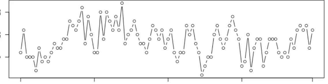
In this thesis, we examine properties of discrete-valued stochastic processes of var-ious forms. As their name suggests, these models constitute a variation of stochastic processes, in which the time-dependent random variables are assumed to take on only nonnegative integer values, i.e., counts. In order to demonstrate some of the defining features, let us present an instructive example of such a data set. In Freeland (1998), the time series plotted in 1.1 is reported, the data originated from the Worker’s Compen-sation Board (WCB) of British Columbia. This organization is tasked with managing the disability benefits for the workers in the heavy manufacturing industry of British Columbia. The data represents the counts of a special subclass of short-term wage loss claims. More precisely, the counts correspond to the number of workers each respective month who received short-term disability benefits due to burn injuries.

● ● ●●● ● ● ● ● ● ● ● ●● ●● ● ● ● ● ● ● ● ● ●● ● ● ● ● ● ● ● ● ● ● ● ● ● ●● ● ● ● ● ● ● ● ● ● ● ● ●● ● ● ● ● ● ● ● ●● ● ● ● ● ● ● ● ● ● ● ● ● ● ● ●● ● ● ●●● ● ● ● ● ● ● ● ● ● ● ● ● 5 10 15 Number of Claims

Jan. 1987 Jan. 1989 Jan. 1991 Jan. 1993 Dec. 1994

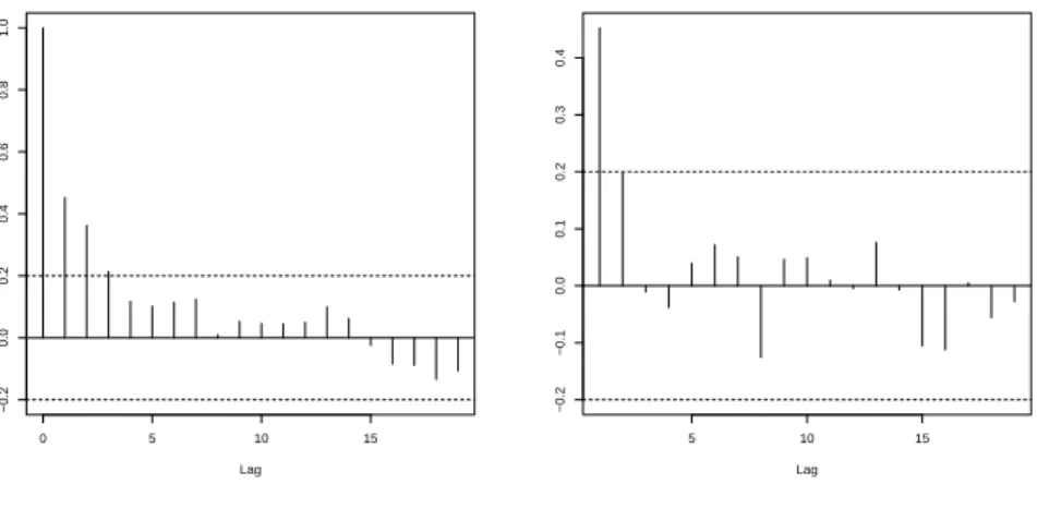
Figure 1.1: Plot of monthly claim counts of workers receiving short-term disability bene-fits after sustaining burn injuries, as reported by the WCB British Columbia. For example, the first two data points show that in January 1987, 6 workers collected short-term disability benefits and in the following month, this number rose to 11. Since burn related injuries take some time to heal, it seems sensible to assume that some of the workers collecting benefits in February were among those counted in January. Thus, the count data should exhibit some form of dependency over time, i.e., it is unlikely that the counts are uncorrelated or even independent. Indeed, the empirical autocorrela-tion funcautocorrela-tion (ACF) and the empirical partial autocorrelaautocorrela-tion funcautocorrela-tion (PACF), plotted in Figure 1.2, uncover a significant deviation of the data from the null hypothesis of independence (dashed lines). For more details on both of these function, see Section 2.6. We are thus faced with the problem of finding a suitable mathematical model for a sequence of counts which allows for serial dependence while its values remain in the range of the nonnegative integersN0. The approaches under consideration in this thesis can be

roughly filed under two categories: The first approach is aninteger-valued analogon to the commonautoregressive model, subsumed by the acronym INAR, the second employs elements of (discrete-time) queueing theory for modeling purposes.

(15)

0 5 10 15 −0.2 0.0 0.2 0.4 0.6 0.8 1.0 Lag ACF of claim counts data

5 10 15 −0.2 −0.1 0.0 0.1 0.2 0.3 0.4 Lag PACF of claim counts data

Figure 1.2: Claim counts for Figure 1.1: Plot of ACF and PACF.

1.1 Integer-Valued Autoregressive Processes

The first approach is motivated by finding similarities in the dependency on the past of the data at hand, y1, . . . , y96 say, with well-known stochastic processes. Looking at the ACF and the PACF in Figure 1.2, the ACF decays exponentially, and the deviation of the PACF from zero is only significant at lag 1. This pattern resembles that of the well known (continuous) autoregressive process of first order (AR(1)) process (see Section 2.6), thus a first approach would be to fit the data of Figure 1.1 to such a model.

However, there are major differences between the data plot in Figure 1.1 and that of an AR(1) process. The realizations y1, . . . , y96 are nonnegative, and they are integer

valued. Both of these characteristics stem from the nature of the data and should be incorporated in an appropriate model. This motivates the introduction of the following integer-valued autoregressive process: Starting with an AR(1) process (Yt)t∈Z satisfying

Yt=αYt−1+t, we need to first make sure that this process is nonnegative and that the realizations are integer-valued, so we assume that t ∈N0 for all t ∈ Z. However, the

multiplication with a value ofα /∈_Z would lead to values outside the integers, yet it is well known that an AR(1) process is only stationary ifα ∈[0,1), where α= 0 pertains to the trivial case of i.i.d. random variables.

Hence, we replace the multiplication with the parameter α ∈ (0,1) with a different operation, the binomial thinning operator of Steutel and Van Harn (1979): If Y is a discrete random variable with range N0 and if α ∈ (0,1), then the random variable α◦X:=PY

i=1Ziis said to arise fromY bybinomial thinning, and theZiare referred to as thecounting series, if they are independent and identically distributed (i.i.d.) Bernoulli random variables with P(Zi = 1) = α, which are assumed to be independent of Y. So each Z satisfies Z ∼Bin(1, α), and α◦Y ∼Bin(Y, α), where Bin(n, π) abbreviates the binomial distribution with parametersn∈Nandπ∈(0,1). Using the random operator

“◦”, let us define the integer-valued autoregressive process of first order (INAR(1)) in the following way.

(16)

Definition 1.1.1 (INAR(1) Model). Let (t)t∈Z be an i.i.d. process with range N0, let

Var[t]<∞ and letα∈(0,1). A process (Yt)t∈Z, which follows the recursion

Yt=α◦Yt−1+t for all t∈Z (1.1)

is said to be an INAR(1) process if all thinning operations are performed independently of each other and of(t)Z, and if the thinning operations at each timetas well as t are

independent of (Ys)s<t.

Let us give an overview of existing literature concerned with the process of Defini-tion 1.1.1 and its extensions. The INAR(1) process owes its denominaDefini-tion to the contri-bution Al-Osh and Alzaid (1987), it was previously suggested as a discretized version of an AR(1) process in McKenzie (1985). Note, however, that very similar processes were already studied earlier in the context of branching processes, see, e.g., Pakes (1971), as the recursion (1.1) may be interpreted as the result of a special branching process, in which each member of the population at time t−1 gives birth to exactly one offspring with probabilityα and does not reproduce with probability 1−α. The older generation then dies out, and an external migration component, distributed ast, enters the popu-lation. This connection to branching process theory is employed in some arguments in this thesis, see for instance the proof of Theorem 4.2.6.

The “◦” operator used in Definition 1.1.1 stems from Steutel and Van Harn (1979), the article which also uncovered the connection of INAR(1) processes and infinite divisibility of random variables, see Theorem 2.3.5. This connection is part of the reasons to consider the special case of Compound Poisson INAR(1) models in Chapters 4 and 5 in such detail, note that the Compound Poisson distributions correspond exactly to the infinitely divisible distributions on N0, cf. Theorem 2.3.3.

In the literature, the interest in INAR processes continued for some time after their introduction. Further results were discussed in Alzaid and Al-Osh (1988) and extension to both higher order INAR processes (see Alzaid and Al-Osh (1990) and Du and Li (1991) as well as Chapter 7) as well as integer-valued ARMA models (see McKenzie (1988)) were introduced. After a short hiatus, the interest began picking up again in the 2000s and the stream of contributions has not dried up since. Especially the application to real data sets has been discussed in a variety of contexts. The dissertation Freeland (1998) and the article Freeland and McCabe (2004) presented data obtained from short term wage loss benefits, one of these time series is presented in Figure 1.1. For a further discussion of these time series, the reader is referred to Section 5.1.3 and Section 6.4.3. In Jung et al. (2005), monthly strike counts published by the U.S. Bureau of Labor Statistics are fitted to an INAR(1) model, for further details we refer to Section 6.4. As a last example, the contribution Weiß (2008) considers this model in the context of download counts of a certain software package, where the number of downloads is counted daily. This list is far from being complete, yet it conveys the message of the versatile applicability of the model (1.1) quite well.

The basic INAR(1) model has been extended in various fashions to comply with ad-ditional considerations. In Zheng et al. (2007), the Random Coefficient INAR(1) model

(17)

is introduced, which allows the parameterαin (1.1) to be a random variable on its own. Another possibility for generalizations consists in allowing for different thinning opera-tions to replace the ”◦” operator, as discussed in Weiß (2008). The higher-order case was also considered in Dion et al. (1995), which emphasized the connection to branching process theory. For details on the approach and the results of the latter reference, the reader is referred to Section 7.2.2. Another topic of discussion is the so-called dispersion of the marginal distribution of the resulting processes as can be seen in Weiß (2009) (for overdispersion) and Weiß (2013) (for underdispersion). This concept is taken up again in Chapters 4 and 5.

In this thesis, a multitude of new research results for INAR(1) processes is presented. One recurring theme is the following question: Having identified the INAR(1) process of Definition 1.1.1 with a certain parametric choice such ast∼Poi(λ) as apossible model for a given data set {y1, . . . , yT}, is it also an appropriate model? No less than four different statistical tests designed to answer this question (or variations of it) are put forward in this thesis. The basic approach remains the same in all four cases: First, an appropriate relation holding under the null hypothesis is identified. Then, an empirical test statistic is constructed which is able to detect deviations from the theoretical value. Finally, the asymptotic behavior of the test statistic is derived, allowing us to evaluate the significance of deviations of the test statistic.

Even though they share one basic approach, the mathematical tools involved in the derivations vary. The first three tests involve relations of joint moments of the processes, and the calculation of these expressions is facilitated by using joint cumulants as shown in Chapter 5. The necessary central limit theorems are derived via the classical notion of strong mixing. The last test of Chapter 6 stands alone, it is also more general than its predecessors. It utilizes empirical generating functions of random variables and is thus able to serve as a goodness-of-fit test for a very large class of processes. The derivation of the necessary central limit theorem does not rely on mixing, but on a more general result for ergodic processes. Furthermore, the convergence in distribution in this case is of a functional type, leading to a much more intricate structure of the proofs.

1.2 Discrete-Time Queueing Processes

A second approach for modeling data as given in Figure 1.1 considers discrete-time queueing models for the underlying process. The history of queueing theory dates back to Erlang (1909) and has since been established as a widely used approach in the assess-ment of real-time events. The main idea behind a single node queueing model is easily explained with the help of a sketch.

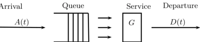
There is a certain arrival stream of customers coming from the outside, denoted by

A(t). Whenever a customer arrives and if at least one server out of a total of N servers is available, the customer begins his service, the length of which is distributed according to some service time distribution G. Should all servers be busy at the time of arrival, the customer is placed in the queue and remains there until he receives service. When-ever a customer has finished his service, he leaves the queue via the departure process

(18)

Arrival Queue Service Departure

A₍t₎ G D₍t₎

Figure 1.3: Sketch of a General Queueing Model

D(t). Such a queueing model can be modeled both in continuous time and with discrete time slots, in this thesis we will always assume the time to be discrete. Concerning notation, the main characteristics of a queueing model are usually summarized in the so-calledKendall notationof the formA/B/c/d. The first entry “A” governs the arrival distribution, the entry “B” the service time distribution and the third, “c” reports the number of servers. The entry “d” denotes the size of the waiting room. This notation may be extended to include more information, for instance, the discipline of the queue (e.g., ”first in, first out” or FIFO) can be added. However, such ramifications will not be necessary in this thesis.

Let us discuss how the data of Figure 1.1 fits into the framework of a discrete-time queueuing system: the time slots are the elapsing months, the arriving customers each month represent the number of workers who suffered an accident involving burn injuries in the course of the current month and now collect short-term wage loss benefits for the first time. The service time corresponds to the duration of the healing period, i.e., the time span in which the worker is ineligible for work due to his injuries. In this scenario, the number of servers is infinite, as there is no (theoretical) limit to the number of workers collecting short-term wage loss benefits. Hence, we are faced with a discrete-time queue in which the arrival is independent, yet general; the service discrete-time is general, as we have no preconception about the healing time of a worker and the number of servers is infinite. In Kendall’s notation, this is a GI/G/∞-queue.

The nonparametric estimation of the service time distribution G within a discrete-time GI/G/∞ queue has been previously considered in a number of publications. In the continuous time case, which can always serve as an orientation, there are the early contributions Brillinger (1974) and Brown (1970), where estimation techniques based on observations of the arrival and departure process is considered. Furthermore, the articles Bingham et al. (1989) and Hall and Park (2004) discuss the nonparametric analysis of the system based on consecutive sequences of busy and idle periods, a related concept and two additional approaches are the topic of Bingham and Pitts (1999). For a detailed literature overview, the reader is referred to Wichelhaus and Langrock (2012).

In discrete time, literature is more scant, notable exceptions are given by Pickands and Stine (1997) where knowledge about the queue length is assumed and Edelmann and Wichelhaus (2014). The results of the latter contribution are discussed in detail below, as they build the vantage point for the analysis of Chapter 3.

In particular, the idea of estimating the sequence of differences as a device to obtain an estimation of the service time distribution was first put forward in Brown (1970),

(19)

refined in Blanghaps et al. (2013) and applied to the discrete time case in Edelmann and Wichelhaus (2014). The idea consist basically in circumventing the main matchmaking problem, i.e., that departures can not be matched to their respective arrivals, by estimat-ing a different distribution first, for which simply (and falsely) any departure is assumed to have been caused by the latest possible arrival. Quite surprisingly, this distribution stands in a very simple relation to the sought after service time distribution. From a mathematical standpoint, both of these distributions may be represented as functionals on the general space of sequencesRN, and the main contribution of Chapter 3 is the proof

of the functional convergence of appropriately chosen estimators of these distributions.

1.3 Bibliographic Notes

Large parts of this thesis are based on a number of published articles of the author in refereed journals. Two of these articles were co-authored by Prof. Dr. Christian Weiß: Schweer and Weiß (2014), Schweer and Weiß (2015). Another article, Schweer and Wichelhaus (2015a), was written in conjunction with Dr. Cornelia Wichelhaus. The published contributions Schweer (2015a) and Schweer (2015b), the latter of which ap-peared in a refereed conference proceedings volume, constitute solo efforts of the author. In order to clarify the origin of the results, the source of each theorem, proposition, lemma etc. is cited. If a theorem or a corollary remains unmarked, it states a new and unpublished result. Unmarked lemmata may state either new results or a well-known assertion, the difference should be clear from the context. In particular, unpublished work can be found in Section 5.3, Section 4.2.4 and Section 7.2.

Concerning notation, this thesis follows the usual mathematical conventions, e.g., denoting the normal distribution with meana and variance b by N(a, b), and so forth. Furthermore, we set N = {1,2,3, . . .} and N0 = N∪ {0}. Denotations exceeding the

scope of the “usual” are defined in the text and listed in the appendix of this thesis for easy reference. In the same place, the reader can find a list of the acronyms and an index of important keywords used in the text.

(20)

(21)

(22)

This chapter gathers together for easy reference a number of useful mathematical concepts used in this thesis. As the focus is put on the collection of established results, most of the proofs are omitted. They are included either if parts of the proof are used in this thesis or if they are slight generalizations of existing results.

The topics of the particular sections vary, beginning with the function-analytic aspects of sequence spaces. These abstract concepts provide the appropriate setting for parts of the analysis in Chapter 3. Next, we discuss some properties of (joint) cumulants, which simplify the explicit calculation of joint moments of INAR(1) processes significantly, see Chapters 4 and 5. Characteristics of Compound Poisson distributions are collected in the next section, these will turn out to be a natural candidate for consideration in the framework of INAR(1) processes. The fourth part of this chapter is concerned with the time-reversibility of stochastic processes, a concept which appears at numerous times throughout this thesis.

The last two sections collect some well-known results for dependent data, the first introduces the classical autocorrelation function and partial autocorrelation function. The second provides two different central limit theorems for dependent data due to Ibragimov (1962) and Billingsley (1999), both of which are employed at multiple times throughout this thesis.

2.1 Sequence Spaces

For the nonparametric estimation of a probability distribution on the real numbers, one usually considers convergence of these estimators in the so-called Skorokhod space

D[−∞,∞]. In this thesis, however, the considered distributions are of a discrete type and it will therefore turn out to be convenient to consider convergence on sequence spaces instead. One such example which we will use extensively is the Banach space

c0 = x= (x1, x2, . . .)∈RN _klim_→∞xk= 0 . (2.1)

We equip this space with the normkxk_c₀ = sup_k_∈_N|xk|. This space is used for proving functional central limit theorems of empirical distribution functions in Henze (1996), the following exposition parallels that of Section 2 of this article.

The σ-algebra of Borel sets of c0 will be denoted by B0, it is generated by the -balls S(x, ) := {y ∈ c0 | kx−ykc0 < }, where x ∈ c0 and > 0. Comparing this with

the smallest σ-algebra onc0 such that the projectionsx 7→ πk◦x :=xk, k∈ N, x∈c0

are measurable, denoted by B, it is easily seen that B = B0_{. Let} _X

n be a mapping from the underlying sample space Ω (with associated σ-algebra A) into c0 for which

πk◦ Xn =: Xn,k is a random variable. It follows that Xn is A-B-measurable, implying that P◦(Xn)−1 is a Borel probability measure on c0. In order to show convergence in

distribution of a sequence to a random element in c0, it is well known that we need to prove the weak convergence of finite-dimensional distributions and verify that the sequence is tight (see, e.g., Billingsley (1999)).

(23)

Recalling that a family of distributions Π is tight if for every > 0 there exists a compact set K such that P(K) > 1− for every P ∈ Π, it is clear that we need to

classify the compact sets in c0. It will turn out to be convenient to consider relatively

compact setsAof c0, for which the closure, denoted by A−, is compact. An-cover is a cover of the space consisting of sets of diameter less than, and a metric space is called totally bounded if it admits a finite -cover for every > 0. The relation between these concepts is the following (cf. Theorem M5 in Billingsley (1999)): Since c0 is a Banach space, the closure of any set is complete, and thus every totally bounded set is relatively compact and vice versa. Let us formulate the key lemma in this context:

Lemma 2.1.1 (Hanche-Olsen and Holden (2010), Lemma 1). Let (X, d) be a metric space and assume that for every > 0, there exists some δ > 0 a metric space (W, d0) and a mapping Φ : X → W such that Φ(X) is totally bounded. Furthermore, assume that whenever x, y∈X are chosen such that d0(Φ(x),Φ(y))< δ, then d(x, y)< . Then

X is totally bounded.

This result allows for a very simple proof of the following assertion. Results of this kind are usually subsumed under the name Arzel`a-Ascoli theorem in honor of Cesare Arzel`a and Giulio Ascoli.

Lemma 2.1.2 (Cp. Henze (1996), Sect.2). A set A⊂c0 is totally bounded if and only if

(i) A is pointwise bounded, i.e., it holds thatsup_x_∈_Akxkc0 <∞.

(ii) for all >0 there exists an N such that sup x∈A

sup k≥N

|xk|< .

Proof. Let us first assume thatAis totally bounded. The existence of a finite-cover for any >0 implies the uniform boundedness ofAand therefore the pointwise boundedness of (i). Now, let > 0 and choose a corresponding cover {U(1), . . . , U(R)} with center pointsy(j)∈U(j). Now chooseN large enough so that

sup k≥N

|y(j)k|< forj= 1, . . . , R,

which is possible sincey(j)∈c0. Letting x∈A be arbitrary, it follows that there exists a y(j) withkx−y(j)k_c₀ < . Using this, we have

sup k≥N |xk| ≤ sup k≥N |xk−y(j)k|+ sup k≥N |y(j)k| ≤2,

proving condition (ii). Now, assume (i) and (ii) hold. Let >0 and choose N as in (ii). Consider the map Φ : A → RN, which maps x to the vector (x1, . . . , xN). Employing the uniform norm k · k∞ on RN, by (i), Φ(A) is totally bounded. Now, assuming that

x, y∈A such that

kΦ(x)−Φ(y)k

RN = sup

k≤N

(24)

we find that kx−ykc0 ≤ sup k≥N |xk−yk|+ sup k≤N |xk−yk|<2,

and an appeal to Lemma 2.1.1 concludes the proof.

This can be translated into the following condition for tightness in the measurable space (c0,B). We repeat the proof shown in Henze (1996) on the one hand to highlight the usefulness of the considerations above and on the other hand to clear the pathway towards possible generalizations.

Lemma 2.1.3(Henze (1996), Lemma 2.1). LetX_n= (Xn,k)_k_∈_Nbe a sequence of random elements of (c0,B). Then Xn is tight if the following two conditions hold:

(i) For each positive δ and l∈_N there is a finite constant M, such that

P(|Xn,l| ≤M)≥1−δ, n≥1. (2.2) (ii) For each positive numbers δ, there exist integers n0 and l0 such that

P sup

k≥l0

|Xn,k|>

!

≤δ for all n≥n0. (2.3)

Proof. The necessity of the conditions is easily seen. Suppose (i) and (ii) hold and let

>0. Let us define the sets

Aj := ( x∈c0 sup k≥l(j) |xk| ≤ 1 j ) ,

wherel(j) is an integer chosen (depending onjand) such thatQn(Aj)≥1−·2−(j+1) for all n. Condition (i) ensures the existence of constants M1, . . . , Ml(1)−1 such that

Q_n(Bk) ≥ 1−/(2(l(1) −1)) for all n, where Bk := {x ∈ c0| |xk| ≤ Mk} for all

k= 1, . . . , l(1)−1. Now, we define A:=B1∩B2∩ · · · ∩Bl(1)−1∩ ∞ \ j=1 Aj,

and with Lemma 2.1.2 it immediately follows from this construction that the closureK

of Ais compact. We calculate Q_n(K)≥1− Q_n(AC)≥ l(1)−1 X i=1 (1− Q_n(Bi)) + ∞ X i=1 (1− Q_n(Ai))≥1−,

(25)

These considerations extendmutatis mutandisto a similar sequence space`1, the space of all absolutely summable sequences, i.e., all sequences (xk)k∈N with

P∞

k=1|xk|< ∞. More precisely, it is easily seen that the results also hold in the space

(`1)2:= ( (x, y)∈_RN_× RN ∞ X k=1 (|xk|+|yk|)<∞ ) ,

equipped with the norm k(x, y)k₍_`₁₎2 = P∞_k₌₁(|x_k|+|y_k|). The corresponding Borel

σ-algebra will be denoted byB₁. We find the following analogon of Lemma 2.1.3:

Lemma 2.1.4. A sequence{Qn}n≥1 of probability measures on((`1)2,B1) is tight if and

only if these two conditions hold:

(i) For each positive δ and eachl1, l2∈N, there exists a finite constant M such that

Qn

x∈(`1)2 | |x1(l1)|+|x2(l2)| ≤M ≥1−δ.

(ii) For each positive δ, η >0, there exists a l0∈_Nsuch that Qn      x∈(`1)2 X k≥l0 (|x1(k)|+|x2(k)|)≤η     ≥1−δ.

2.2 Cumulants

The following exposition resembles that of Section 2.3 in Brillinger (1981) closely. Let us consider a r-variate random variable (Y1, . . . , Yr) with E[Yir]<∞ for alli∈ {1, . . . , r}. We define the r-th order joint cumulant cum(X1, . . . , Xr) as follows:

cum(Y1, . . . , Yr) = X π∈Πr (−1)|π|−1(|π| −1)! |π| Y i=1 E   Y l∈Bi(π) Yl  , (2.4)

where Πr is the set of all possible partitions π of the set {1, . . . , r}, |π| denotes the number of blocks in a partitionπ andBi(π) denotes thei-th block in said partition, i.e.,

S

iBi(π) = {1, . . . , r}. A special case of (2.4) is given for Yi = Y, then the definition reduces to that of therth order cumulant of a random variableY, which we will denote by κr(X) throughout this thesis. We now summarize the following properties:

Lemma 2.2.1(Brillinger (1981), Theorem 2.3.1). Let(Y1, . . . , Yr)be ar-variate random variable with E(Yir)<∞ for all i∈ {1, . . . , r}. Then

(i) If Yi=Y for all i∈ {1, . . . , r}, then cum(Y, . . . , Y) =κr(Y).

(ii) If any group ofYi’s is independent of the remainingYj’s, thencum(Y1, . . . , Yr) = 0. (iii) The cumulant function is additive, i.e., cum(Y1+Z1, . . . , Yr) = cum(Y1, . . . , Yr) +

(26)

(iv) cum(a1Y1, . . . , arYr) =a1· · ·arcum(Y1, . . . , Yr) for a1, . . . , ar constant.

(v) If r ≥2, then the r-th order joint cumulant is shift-invariant, i.e., for constants

c1, . . . , cr ∈R it holds that cum(Y1+c1, . . . , Yr+cr) = cum(Y1, . . . , Yr). (vi) For any r∈_N,

E[Y1· · ·Yr] = X π∈Πr |π| Y i=1 cum(YBi(π)),

where Πr andBi(π) are as in (2.4)and where YBi(π)= (Ybi(π,1), . . . , Ybi(π,p)), with Bi(π) ={bi(π,1), . . . , bi(π, p)}.

(vii) Let X1,i, X2,i, . . . , Xr,i be sequences of nonnegative random variables, such that

Xi,j and Xk,l are independent for j 6= l for all i, k ∈ {1, . . . , r} and such that

E[(P∞i=0Xj,i)r]<∞ for j∈ {1, . . . , r}. Then cum ∞ X i=0 X1,i, ∞ X i=0 X2,i, . . . , ∞ X i=0 Xr,i ! = ∞ X i=0 cum (X1,i, X2,i, . . . , Xr,i).

Proof. For (i) through (v), we refer to (Brillinger, 1981, Theorem 2.3.1), relation (vi) is well-known. Concerning (vii), as the conditionE[(P∞i=0Xj,i)r]<∞ ensures that the

expression is well-defined (Brillinger, 1981, Definition 2.3.1), we prove this statement via application of the defining equation (2.4) of joint cumulants. In order to allow for the changing of the order of integration (i.e., taking the mean) and summation, we apply Lesbesgue’s monotone convergence theorem. Since the Xji’s are nonnegative and since the arising expectations have an upper bound in max1≤j≤r{E[(P∞i=0Xji)r]}<∞, this theorem is applicable. We first find with (iii) that

cum ∞ X i1=0 X1,i, ∞ X i2=0 X2,i, . . . , ∞ X ir=0 Xr,i ! = ∞ X i1=0 cum X1,i1, ∞ X i2=0 X2,i, . . . , ∞ X ir=0 Xr,i ! =. . .= ∞ X i1=0 · · · ∞ X ir=0 cum (X1,i1, X2,i2, . . . , Xr,ir),

which, using (ii), concludes the proof.

To give a better feeling for what cumulants do, notice that cum(X, X) = Var(X) as well as cum(X, Y) = Cov(X, Y) provided the respective moments exist. Thus, cumulants are close relatives of joint moments with rather nice mathematical aspects such as multi-linearity. This makes their application in situations where the random variables in question carry a lot of structure quite advantageous in comparison to the calculation of raw joint moments. This is used, e.g., in the proof of Lemma 5.2.2 below.

Let us further record that the concept of overdispersion, which will be of great im-portance throughout this thesis, can also be stated in terms of cumulants. Theindex of

(27)

dispersion of a random variable X is defined as

IX :=

Var(X)

E[X] . (2.5)

If IX = 1 (for instance in Poisson distributions), X is equidispersed, if it is larger than 1 then X is overdispersed. For IX < 1 the term underdispersed is used. In terms of cumulants, this may be expressed via the fractionκ2(X)/κ(X).

After this side note, let us continue with the law of total cumulance. This was intro-duced in Brillinger (1969) and is restated below. It extends the law of total expectation

E[X] = E[E[X|Y]] and law of total variance Var(X) = E[Var(X|Y)] + Var(E[X|Y])

(whereX, Y are random variables on the same probability space with finite moments of appropriate order) to cumulants:

Theorem 2.2.2 (Brillinger (1969), Theorem 1). Let (Y1, . . . , Yr) be a r-variate random variable with E(Yir) <∞ for all i∈ {1, . . . , r} and let X be a random variable defined on the same probability space as the Yi’s. Then

cum (Y1, . . . , Yr) = X π∈Πr

cum cum(YB1(π)|X), . . . ,cum YBp(π)|X

,

where Πr, Bi(π) and YBi(π) are as in Lemma 2.2.1 (vi).

2.3 Compound Poisson Distributions

The following exposition is very closely modeled after the corresponding section of the Appendix of Schweer and Weiß (2014). For the Compound Poisson distribution, we adapt the notations and definitions from Chapter XII in Feller (1968).

Definition 2.3.1 (Compound Poisson Distribution). Let X1, X2, . . . be i.i.d. random

variables with rangeNand probability generating function (pgf )H(z), the compounding

distribution, whereν := deg(H(z)). LetN be Poisson distributed with meanλ >0, i.e.,

N ∼Poi(λ), independently ofX1, X2, . . . Then:=X1+. . .+XN is Compound Poisson distributed, denoted by ∼ComPoiν(λ, H). The pgf of is given by

pgf(z) = exp (λ(H(z)−1)). (2.6) The distribution of Definition 2.3.1 has also been referred to as Poisson-stopped sum distribution, stuttering Poisson distribution, multiple Poisson distribution (John-son et al., 2005, Sections 4.11 and 9.3), and as extended Pois(John-son distribution of orderν

if ν <∞ in Aki (1985). The ComPoiν-distribution includes several well-known distri-butions as a special case. It is equidispersed if and only if ν = 1, and overdispersed otherwise. Furthermore, the Compound Poisson distributions are closely linked to the infinitely divisible distributions, defined as follows.

Definition 2.3.2 (Infinite Divisibility). Let H be a probability distribution on N0 with

pgf_X(z) = H(z). Then H is infinitely divisible, if for each positive integer n, the n-th root, pn

(28)

Whereas this definition uses pgfs for its formulation, one could equivalently define: H

is infinitely divisible if for eachn∈_Nthere existni.i.d. random variables X1n, . . . , Xnn such that X1n+· · ·+Xnn ∼H. The link between such distributions and Compound Poisson distributions is given by the next result.

Theorem 2.3.3 (Feller (1968), Sect. XII.2). Let G be a probability distribution on N0

with pgfG(z). Then the following statements are equivalent: (i) G is infinitely divisible,

(ii) there exist λ >0 and a pgf H(z) such that G∼ComPoi(λ, H), (iii) G(1) = 1and logG(z) G(0) = ∞ X i=1 aizi, where ak ≥0, ∞ X i=1 ak <∞.

There is another classification for these distributions that we want to mention here. Let us first introduce the notion of discrete self-decomposability.

Definition 2.3.4 (Discrete Self-Decomposability). Let H be a probability distribution onN0 with pgfH(z). ThenH isdiscrete self-decomposable (DSD), if for eachα∈(0,1)

there exists a pgf Hα(z) such that

H(z) =H(1−α+αz)Hα(z). (2.7) In Steutel and Van Harn (1979), the following deep result is shown.

Theorem 2.3.5 (Steutel and Van Harn (1979), Theorem 2.2). Let G be a probability distribution on N0 with pgf G(z). Then G is discrete self-decomposable if and only

if G is infinitely divisible with G ∼ ComPoi(λ, H), where the sequence (n·hn)n∈N is

nonincreasing.

Proof. The entire assertion is contained in the cited reference, we only show that for the canonical measure (rn)n∈N we have rn=λ(n+ 1)hn+1 for all n∈N. We calculate

− Z 1 z ∞ X n=0 rnundu= ∞ X n=0 rn n+ 1 −1 +z n+1 =λ(H(z)−1).

The latter equality, together with elementary characteristics of power series concludes the proof.

Example 1 (Poisson Distribution of Orderν, Negative Binomial Distribution).

If ν <∞ and if the compounding distribution is the uniform distribution on{1, . . . , ν}, i.e., if hx = 1/ν for all x= 1, . . . , ν, then the resulting distribution is also known as the Poisson distribution of order ν, see Sections 9.3 and 10.7.4 in Johnson et al. (2005). This distribution is abbreviated hereafter as Poiν(λ), where Poi1= Poi.

(29)

Also the negative binomial distribution NegBin(n, π) with n > 0 and π ∈ (0,1) is Compound Poisson, withλ:=−nlnπ and hk= (1−π)k/(−klnπ) for allk∈N. Here,

the Xi of Definition 2.3.1 follow the logarithmic series distribution LSD(π) (Johnson et al., 2005, Chapter 5).

The requirement in Definition 2.3.1 that theX1, X2, . . . have the rangeN={1,2, . . .}

guarantees a unique representation of the associated Compound Poisson distribution. This follows from (2.6) and

exp (λ(H(z)−1)) = exp λ(h0−1 +h1z+h2z2+. . .) = exp λ(1−h0) −1 + h1 1−h0 z+ h2 1−h0 z2+. . . ,

which implies that for each choice ofλ0 >0 and H0(z) withh0₀ >0 there exists aλ >0 and aH(z) with h0 = 0 such that ComPoi(λ0, H0)

D

= ComPoi(λ, H), as equality of the pgfs implies equality in distribution. Thus, without loss of generality, we may assume

H(0) = 0 throughout this thesis, cp. p. 389 in Johnson et al. (2005).

The following two assertions are concerned with the raw moments of Compound Pois-son distributions, so we first introduce some notation. Throughout this thesis, the moments about the origin of a random variable are abbreviated as µ,k := E[k] with

µ:=µ,1. The central moments are denoted as ¯µ,k :=E[(−µ)k], with σ2:= ¯µ,2.

Proposition 2.3.6(Schweer and Weiß (2014), Proposition B.1). LetbeComPoi(λ, H )-distributed according to Definition 2.3.1.

(i) A recursive scheme for the computation of P(=s) is given by

P(= 0) =e−λ, sP(=s) =λ

s−1

X

j=0

(s−j)hs−jP(=j) for s≥1.

(ii) If the moments µX, r of Xi exist, then the cumulants of are given by

κ,r =λµX, r.

Part (i) was derived by Kemp (1967); an explicit expression for P(=s) is given on

p. 288 in Feller (1968). Part (ii) is considered in Section 2 of Aki et al. (1984), it follows immediately from the cumulant generating function (cgf) cgf(z) =λ(H(ez)−1), also see relation (2.6), where H(ez) is just the moment generating function (mgf) of Xi. Note that part (ii) implies that the index of dispersion ofequalsE[X12]/E[X1], i.e., the

ComPoiν-distribution is equidispersed if and only ifν = 1, and overdispersed otherwise.

Example 2 (Poisson Distribution of Order ν). Let ∼ Poiν as given in Example 1. Since the Xi are uniformly distributed, the raw moments µ,r = 1_νPνx=1xr are easily

(30)

computed, and from Proposition 2.3.6 (ii), we immediately obtain the cumulants of. In particular, ¯ µ,1= λ(ν+ 1) 2 , µ¯,2 = λ(ν+ 1)(2ν+ 1) 6 , µ¯,3 = λν(ν+ 1)2 4 , ¯ µ,4= λ(ν+ 1)(2ν+ 1)(3ν2+ 3ν−1) 30 + 3σ 4 . (2.8)

For further details on the relations between moments and cumulants, the reader is re-ferred to Appendix 7 in Douglas (1980).

Example 3 (Negative Binomial Distribution). The negative binomial distribution with parameter (n, π) of Example 1 satisfies

¯ µ,1= n(1−π) π , µ¯,2 = n(1−π) π2 , µ¯,3 = n(1−π)(2−π) π3 , ¯ µ,4= 3n2(1−π)2+n(1−π)(π2−6π+ 6) π4 . (2.9)

For these and further properties of the NegBin(n, π)-distribution, we refer to Chapter 5 in Johnson et al. (2005).

Another popular member of the ComPoi∞-family is Consul’sgeneralized Poisson

dis-tribution (also Lagrangian Poisson distribution), GP(θ, η), see Zhu and Joe (2003) and Section 7.2.6 in Johnson et al. (2005) for details. Here, the compounding probabilities are given by hx =η(ηx)x−1e−ηx/x!, see Example 5.5. in Zhu and Joe (2003).

2.4 Time-Reversibility of Stochastic Processes

The concept of time-reversibility of stochastic processes will be of interest during various stages of this thesis. Formally, a process is time-reversible if it obeys the following definition.

Definition 2.4.1 (Time-Reversibility). A stochastic process (Yt)t∈_Z is time-reversible

if the vector (Yt1, Yt2, . . . , Ytn) has the same distribution as (Yτ−t1, Yτ−t2, . . . , Yτ−tn) for

allt1, t2, . . . , tn, τ ∈Z.

In order for a process to be time-reversible it should exhibit the same behavior whether time passes normally or ”backwards”, or, to put it more eloquently,

Speaking intuitively, if we take a film of such a process and then run the film backwards the resulting process will be statistically indistinguishable from the original process.

(31)

The criterion given in the definition is formulated for general stochastic processes. If the underlying structure of the process is simpler, e.g., Markovian, the necessary and sufficient conditions for time-reversibility can be stated much more succinctly, as shown by Kolmogorov’s criterion.

Theorem 2.4.2 (Kelly (1979), Theorem 1.7). A stationary Markov chain (Yt)t∈Z on a

discrete state space S is time-reversible if and only if the transition probabilities, given by P(Yt=l | Yt−1=k) :=pY(l|k) satisfy the relation

It should be noted that time-reversibility of a process is a very rare characteristic among stochastic processes. On the other hand, the time-reversible models are often the most popular models. As an example, Weiss (1975) shows that the continuous AR(p) process is time-reversible if and only if it is Gaussian, a very widely used model. Since the question whether a given process is Gaussian is a crucial one in time series analysis, this observation has lead to the following specification test by Ramsey and Rothman (1996): Suppose that the process is time-reversible, then it necessarily holds thatE[YtiY

j

t−k] =E[Y j

t Yti−k] for anyi, j, k ∈N.In particular, in later parts of this thesis, (see Section 5.2) we will be interested ingeneralized autocovariance function β(·) defined by β(k) :=EYt2Yt−k −EYtYt2−k fork∈N. (2.10)

If (Yt)t∈_Z is time-reversible, it follows that β(k) = 0 for all k ∈ N0. The empirical

counterpart of β(·), computed from an observation Y1, . . . , YT of a stationary process (Yt)t∈_Z, is defined as ˆ βT(k) := 1 T−k T X t=k+1 Y_t2Yt−k−Yt2−kYt fork∈ {1, . . . , T1}. (2.11)

The resultant test for time-reversibility of (Yt)t∈Z checks the deviation of ˆβT(k) from 0.

2.5 Central Limit Theorems for Dependent Data

At various instances throughout this thesis, we will be interested in deriving central limit theorems (CLTs) for diverse functionals of discrete time series. The usual approach for such theorems is the following: Supposing that the random variables Y1, . . . , YT are identically distributed and independent, have mean zero and a finite variance σ2, it is easily shown using characteristic functions (or similar techniques), that the convergence

1

√

T

P

Yi → N(0, σ2) holds in distribution. For the data we study in this thesis, however, the assumption of independence is too strong as we want to allow the processes to depend on their past realizations, hence the need for central limit theorems for dependent random

(32)

variables. Note that the processes studied in this thesis are stationary as a rule, hence the assumption of identically distributed random variables is not violated.

The general idea behind central limit theorems for dependent data usually boils down to the assumption that the data, while dependent over time, become “more and more” independent the further the data points are apart. In order to measure the level of dependency within the data for a given stationary stochastic process (Yt)t∈_Z, we define

the notion of strong mixing.

Definition 2.5.1 (α-Mixing). Let (Yt)t∈Z be a stationary stochastic process and define

the σ-algebras F_k(Y) := σ(Yi ;−∞ < i ≤ k) and Fl(Y) := σ(Yi ;l ≤ i < ∞). Then (Yt)t∈_Z is α-mixing, if

αY(n) := sup

A∈Fk(Y);B∈Fk+n(Y)

|_P(A∩B)−_P(A)P(B)| →0 as n→ ∞. (2.12)

For each n ∈ N, the coefficient appearing in (2.12) are called α-mixing or strong

mixing coefficients (or weights). The notion of strong mixing is usually credited to Rosenblatt (1956), and it should be pointed out that the number of different types of mixing formulations has increased since then, necessitating specializations such as α -mixing or β-mixing. Indeed, the excellent survey paper on mixing properties Bradley (2005) lists no less than eight different types of strong mixing conditions. In this thesis, we will make frequent use of the following central limit theorem forα-mixing stationary processes.

Theorem 2.5.2 (Ibragimov (1962), Theorem 1.7). Let (Yt)t∈Z be a stationary and α

-mixing process withE[|Y0|2+δ]<∞ for some δ >0 and where

∞ X j=1 (αY(j)) δ 2+δ _<∞_. _(2.13)

Then the series σ2 =P

j∈_ZCov(Y0, Yj) converges absolutely, and √ T 1 T T X i=1 Yi−E[Y0] ! D → N(0, σ2).

One of the reasons why α-mixing has gained such an importance is that it is invariant under measurable maps, i.e., if (Yt)t∈_Zis anα-mixing process andf is a measurable map,

then the process (f(Yt))t∈_Z isα-mixing again. On the other hand, mixing conditions are

often difficult to verify directly. An alternative criterion is used in the following result. For the first assertion we provide a sketch of the proof given in the cited reference, as some of the arguments will be used again at later stages of this thesis.

(33)

Theorem 2.5.3 (Billingsley (1999), Theorem 19.1). Let (Yt)t∈Z be a stationary and

ergodic process withE[Y02]<∞. Let

∞ X j=1 k_E[Yj−E[Y0]| F0(Y)]k_L2 <∞, (2.14) wherekXk_L2 = (_E[|Y|2]) 1

2 denotes theL2 norm. Then the seriesσ2 =P

j∈ZCov(Y0, Yj)

converges absolutely, and √ T 1 T T X i=1 Yi−E[Y0] ! D → N(0, σ2).

Proof. without loss of generality, E[Y0] = 0. By the Cauchy-Schwarz inequality,

|_E[Y0Yi]| ≤E[|Y0| · |E[Yi|F0(Y)]|]≤ kY0kL2· k_E[Y_i|F₀(Y)]k_L2, (2.15)

thus (2.14) shows that the series σ2 converges absolutely. The stationarity of (Yt)t∈Z

implies thatE[(Pni=1Yi)2] =nE[Y02] + 2

Pn−1

i=1(n−i)E[Y0Yi]. Direct calculations yield

∞ X i=−∞ E[Y0Yi]− 1 nE   n X i=1 Yi !2  ≤2 ∞ X i=n |_E[Y0Yi]|+ 2 n n−1 X i=1 ∞ X l=i |_E[Y0Yl]|, (2.16)

which implies _n1E[(Pn_i₌₁Yi)2]→σ2. For the former series in (2.16) the convergence to

and notice that limn→∞ n−_nj = 1 for eachj∈Nwhich, due to the dominated convergence

theorem, yields the result.

The condition (2.14) can be seen as an alternative form of the mixing condition (2.12), in the sense that, under this condition, the dependence of the process on a given reference stateY0 decays fast enough to 0 to be summable in the L2 norm. The advantage of this

condition in comparison to mixing conditions is that the conditional expectation is more easily accessible if the structure of the process is simple. A useful inequality in the context of (2.14) is given in the following Lemma, a consequence of Jensen’s inequality.

Lemma 2.5.4(Billingsley (1999), eq. (19.25)). LetX be a random variable on(Ω,A,P)

with a finite second moment and let M and N be σ-algebras satisfying M ⊂ N ⊂ A. Then

(34)

2.6 Autocovariance Function and Related Concepts

In order to assess the dependence of a given stochastic process on the past, there is a multitude of functions available. In this section, we consider the three most popular functions, the autocovariance function γ(·), the autocorrelation function ρ(·) and the partial autocorrelation functionρpart(·). For a given stationary process (Yt)t∈_Z, the first

two functions are easily defined:

γ(k) := Cov (Yt, Yt+k) and ρ(k) :=

γ(k)

γ(0) fork∈Z. Denoting Y := _T1 PT

i=1Yi, the empirical counterparts are also easily established:

b γ(k) := 1 T −k T−k X i=1 Yi−Y Yi+k−Y and ρb(k) := b γ(k) b γ(0) fork∈ {0, . . . , T −1}.

Let us give an example. Letp∈Nand letα1, . . . , αp∈(−1,1) denote appropriately cho-sen parameters, then a stationary stochastic process is called a continuousautoregressive process of order pif it satisfies the recursion

Yt= p

X

i=1

αiYt−i+t, (2.18) where (t)t∈_Z is a sequence of white noise random variables (note that in this case, t can take on values in R). Since E[0] = 0 it follows that E[Y0] = 0, and multiplication

of (2.18) with Yt−k on both sides and taking expectations γ(k) =

Pp

i=1αiγ(k−i) for any k∈_N, the Yule-Walker equations. For instance, if (Yt)t∈_Zis an AR(1) process with

parameterα ∈(−1,1), these immediately implyγ(k) =αkγ(0) for all k∈N0 and thus ρ(k) =αk. The partial autocorrelation function is a little harder to define. Essentially,

ρpart(k) evaluates the correlation of the random variables Yt and Yt+k adjusted for the intermediate values Yt+1, . . . , Yt+k−1.

Definition 2.6.1(Partial Autocorrelation Function). Let(Yt)t∈Zbe a stationary process

with E[Y02] < ∞ and autocorrelation function ρ(·). Then ρpart(·) is called the partial autocorrelation function if it satisfies ρpart(1) :=ρ(1)and ρpart(k) = det(Uk)/det(Lk), where the matrices (for k≥2) are given by

Uk :=      1 ρ(1) . . . ρ(k−2) ρ(1) ρ(1) 1 . . . ρ(k−3) ρ(2) .. . . .. ... ... ρ(k−1) . . . ρ(1) ρ(k)      ,Lk :=       1 . . . ρ(k−1) ρ(1) . .. ρ(k−2) .. . ... ρ(k−1) . . . 1       .

It is quite obvious that ergodicity of the process together with appropriate moment assumptions already yields consistency of the estimators _bγ(k) for any k∈ _N₀, and the

(35)

continuous mapping theorem immediately implies the consistency ofρb(k) and ρbpart(k).

for any k∈_N.

The asymptotic normality of the estimators can be treated similarly. If suffices to show that the estimators for the autocovariance functionγ(·) are jointly asymptotically normal to provide inference for the asymptotic behavior of the ACF and PACF estimators. We record this result together with two important consequences.

Theorem 2.6.2(Romano and Thombs (1996), Theorem 3.2). Let(Yt)_t_∈_Zbe a stationary process with _√

T(_bγ(0)−γ(0), . . . ,_bγ(K)−γ(K))→ ND (0,T+U),

where the entriesτi,j of the matrix T are given by

τi+1,j+1 =

∞

X

d=−∞

[γ(d)γ(d+j−i) +γ(d+j)γ(d−i)],

and where the entries ui,j of the matrix U are given by

ui+1,j+1 =

∞

X

d=−∞

cum(Y0, Yi, Yd, Yd+j).

Let q ≥1 and denote K :=p+q. Then √

T(ρb(1)−ρ(1), . . . ,ρb(K)−ρ(K))

D

→ N 0,T0+U0,

where the entries of the matrixT0 are calculated from Tvia

τ_i,j0 = 1

γ(0)2(τi+1,j+1−ρ(i)τ1,j+1−ρ(j)τi+1,1+ρ(i)ρ(j)τ1,1),

analogously for the matrix U0.

In the special case of autoregressive processes, we are able to explicitly calculate the resulting covariance matrix of the estimator of the partial autocorrelation function.

Theorem 2.6.3 (Ku and Seneta (1996), Theorem 1). Let (Yt)t∈Z satisfy the conditions

of Theorem 2.6.2 and let the ACF satisfy the Yule-Walker equationsPp

j=0αjρ(i−j) = 0,

where α0:=−1 and where Ppi=1|αi|<1. Then √

T(ρ_bpart(p+ 1), . . . ,ρbpart(K))

D

→ N (0,1q×q+Λ), where 1q×q is the unity matrix and the entries of Λ are given by

di,j = 1 γ(0)2₍Qp i=11−ρpart(i)2)2 2p X u=0 X m+n=u αmαn 2p X r=0 X s+t=r αsαtup+1+i−r,p+1+j−u.

(36)

Proof. In (Ku and Seneta, 1996, Theorem 1), it is shown that if the random vector √

T(ρ_b(1) −ρ(1), . . . ,ρ_b(K)− ρ(K)) converges in distribution to some random vector (V(1), . . . , V(K)), then the random vector √T(ρ_bpart(p+ 1), . . . ,ρbpart(K)) converges in

distribution to the vector (W(p+ 1), . . . , W(K)), where

W(k) = Pp m=0 Pp n=0αiαjV(k−m−n) Qp i=1(1−ρpart(i)2) . (2.19)

Here,V(0) := 0 and V(−k) :=V(k) for k≥1. The conditions are obviously fulfilled in our case, and we further have E[V(k)] = 0 for each k ∈Z. Using the approach of Ku

and Seneta (1996), we first write

V:= (V(p+q), . . . , V(−p+ 1))>,W:= (W(p+ 1), . . . , W(p+q))> and theq×(2p+q) matrixA:=A0/(Qp

i=1(1−ρpart(i)2)), where A0 :=      0 . . . 0 1 P 1αmαn . . . P2pαmαn 0 . . . 1 P 1αmαn . . . . P 2pαmαn 0 .. . ... 1 P 1αmαn . . . . P 2pαmαn 0 . . . 0      ,

where summing from 1, i.e., means form+n= 1. With these notations, we may write (2.19) asW =AV, noticing that p X m=0 p X n=0 αiαjV(k−m−n) = 2p X u=0 X m+n=u αiαjV(k−u).

AsVhas a multivariate normal distribution with mean 0 so doesW. Let the covariance matrix ofW be denoted by ΣW, then Theorem 2.6.2 implies ΣW =AT0A>+AU0A>.

In Ku and Seneta (1996) it is shown that AT0A> = 1q×q, the entries of Λ remain to

be calculated. For this, we introduce the convenient functions (cp. eq. (3.4) in Ku and Seneta (1996) and Property 3 in Choi (1990))

h(k) = 2p X u=0 X m+n=u αmαnρ(k−u), (2.20)

withh(k) = 0 fork=p, p+ 1, . . .. Theorem 2.6.2 implies thatdi,j equals, omitting the constant factors, = 2p X u=0 X m+n=u αmαn 2p X r=0 X s+t=r αsαtup+1+i−r,p+1+j−u+h(p+i)h(p+j) −h(p+i) 2p X u=0 X m+n=u αmαnu1,p+1+j−u−h(p+b) 2p X r=0 X s+t=r αsαtup+1+i−r,1, cp. p. 627 in Ku and Seneta (1996), concluding the proof.

(37)

3 Nonparametric Estimation in

Discrete-Time Queueing

(38)

The problem under consideration in this chapter is the estimation of the cumulative distribution function (cdf) of the service time distributionGin a discrete-timeGI/G/ ∞-queue, i.e., a queueing model with an infinite number of servers, a general service time distribution and a general i.i.d. batch arrival process (A(t))t∈Z. We assume that the

available information about the behavior of this queue consists only of the counts of arrivals (A(t))t∈_Z and departures (D(t))t∈_Z from the queue in each time slot. More

pre-cisely, we consider a queue in which there is no possibility for the observer to distinguish between any of the customers, so that the matching of any departure to its respective arrival is impossible. Additionally, the number of customers present at the beginning of the observation is also unavailable. Our goal is the estimation of the entire service time distribution for which we assume no parametric form of any kind. Thus we are faced with a nonparametric estimation problem for G, for which we merely assume a finite mean and that its range is contained in N.

The solution we present to this problem in this chapter starts out with the nonpara-metric estimation of a different distributionH and uses the surprisingly simple relation betweenGand H. The nonparametric nature of the estimates necessitates the applica-tion of funcapplica-tional approaches to the problem, which will be assumed to take place in the sequence space c0. Since the resultant asymptotic expressions are rather involved and depend on unknown parameters, a bootstrapping procedure is suggested and is shown to be a viable option in our context under mild additional conditions. This chapter is an extended version of the article Schweer and Wichelhaus (2015a).

3.1 Introduction and Statement of the Problem

We begin by precisely defining the queueing model and stating the first results. The behavior of the queue is modeled as follows: denote the number of arrivals in thet-th time slot, the time slot between timetandt+ 1, byA(t) and the number of departures in this slot byD(t). In each time slott∈Z, indistinguishable customers labeledKt,1, . . . , Kt,A(t)

arrive, where A(t) = 0 is interpreted as no customers arriving in the t-th time slot. We assume that the sequence (A(t))t∈_Z is i.i.d., has range N0 and that E[A(0)] < ∞.

Each customerKk,j receives upon arrival a sojourn timeSk,j independently of all other customers arriving or present at the queue, whereSk,j is distributed with cdfG(·), which has range N and a finite mean, i.e. P∞i=1(1−G(i)) < ∞. Denoting the probability

masses of the distribution G by gj for j ∈ N, we thus have P(Sk,j = l) = gl for any

k∈_Z,j, l∈_N. Each customerKk,j then remains in service exactly the number of time steps that his service time Sk,j demands and then leaves the queue. We point out that we make the assumptionG(0) = 0 in order to ensure that each customer remains in the queue for at least one time step. We limit our knowledge about the considered system to the sequences (A(t))t∈_Z and (D(t))t∈_Z and we base our analysis of the behavior of

this system solely on this information, i.e., we do not assume to have any possibility of matching the arrival of certain customers to their respective departures.

We define the “enlarged” process (ξ(t))t∈Z byξ(t) :={St,1} × {St,2} × · · · × {St,A(t)},

(39)

carries information about both the number of arrivals in the t-th time slot as well as the service time distribution for these arrivals. Notice that ξ(t) ∈ _NN_{∪ {0}} _{for each}

t∈_Z, where the state 0 represents the case of no arrivals in thet-th time slot. Since the sequences of random variables (Sk,·)k∈Zand (A(t))t∈Zare i.i.d., it follows that the process

(ξ(t))t∈Z is stationary and ergodic. Furthermore, recall the definition of theσ-algebras

F_k(ξ) :=σ(ξ(i) ;−∞< i≤k) for k∈_Zas in Section 2.5. With this construction, the process (ξ(t))t∈Z is an element of the space {NN∪ {0}}Z. We consider this Baire space

to be endowed with its product topology, and we denote the Borel-σ-algebra based on the open sets of this topology byF∞(ξ).

Under the assumption that the system has started in the infinite past, it follows from the construction of the process that we may express the queue length Y(t), i.e., the number of customers in service during thet-th time slot by

Y(t) = ∞ X j=0 A(t−j) X l=1 1{St−j,l>j}, (3.1)

where customers who leave during the t-th time slot are not considered to be in ser-vice. From this representation and the assumption that the sequences (Sk,·)k∈_Z and

(A(t))t∈_Z are i.i.d., it follows that the queue length process is stationary. Furthermore,

the application of Wald’s equation (see (3.2) below) implies that under the assumption of a finite mean of both service time distribution and arrival distribution, the stationary distribution of the queue length process has a finite mean. Finally, we remark that we may express the departure process as follows

D(t) = ∞ X j=1 A(t−j) X l=1 1{St−j,l=j}.

Let us first record some important relations. First, a well-known result due to Wald as well as Blackwell and Girshick states that if T, X1, X2, . . . are independent random variables with finite variance, and if T has rangeN0 and theX1, X2, . . . are identically

distributed, then, withST :=PTi=1Xi,

E[ST] =E[T]E[X1] and Var (ST) =E[X1]2Var(T) +E[T] Var(X1). (3.2)

The former relation is called Wald’s equation. As immediate consequences of these relations, we find that, for all t∈_Z,

E[D(t)] = ∞ X j=1 E   A(t−j) X l=1 1{St−j,l=j}  =E[A(0)] ∞ X j=1 gj =E[A(0)].

We used that the sequence (A(t))_t_∈_Z is i.i.d. and the monotone convergence theorem. Furthermore, ifE[A(0)2]<∞, Var(D(0)) = ∞ X j=1 Var   A(−j) X l=1 1{S−j,l=j}  = ∞ X j=1 E[A(0)]gj(1−gj) +gj2Var(A(0)) .

(40)

Notice that max{E[A(0)],Var(A(0))} ≤maxE[A(0)],E[A(0)2] , and since the random

variable A(0) is discrete-valued, maxE[A(0)],E[A(0)2] = E[A(0)2]. We may thus

conclude that Var(D(0))≤2E[A(0)2] and Var D(0)1{Z(0)≤x}

≤_E[D(0)2]<∞.

Additionally, we note that in the popular case of Poisson distributed arrivals it holds that Var(A(0)) =E[A(0)] and hence Var(D(0)) = Var(A(0)). Furthermore, in this case

we easily calculate, for s6= 0,

Cov (D(0), D(s)) = ∞ X j1=1 ∞ X j2=1 Cov   A(−j1) X l=1 1{S−j₁,l=j1}, A(s−j2) X l=1 1{Ss−j₂,l=j2}   = ∞ X j1=1 gj1gj1+s E[A(0) 2_]₋ E[A(0)]−E[A(0)]2= 0, (3.3)

a quite surprising result. In order to give an explanation for this curious result, we need to consider the time-reversibility of the process.

3.1.1 Time-Reversibility of the Queue Length Process

We now show that the special case of Poisson distributed arrivals A(t) leads to a time-reversible queue length process (Y(t))t∈_Z. Let us remark that this result was already

mentioned in passing in Pickands and Stine (1997) but no formal proof was given.

Lemma 3.1.1(Cp. Pickands and Stine (1997), Sect. 2). Let A(t)∼Poi(λ) for allt∈Z

and some λ >0 and let P∞

i=1(1−G(i))<∞. Then (Y(t))t∈Z is time-reversible.

Proof. The finiteness of the expected service time immediately implies finiteness a.s. of (Y(t))t∈_Z. Let b(ta;tb1, tb2) denote the number of customers arriving at the system in

time slotta and departing in between the time slots tb1 and tb2 with ta≤tb1 ≤tb2. We

first notice that (settingta= 0 without loss of generality)

P r X l=1 1{S0,l∈{tb₁,...,tb₂}}=s ! = r s   tb₂−tb₁ X l=0 gtb₁+l   s 1− tb₂−tb₁ X l=0 gtb₁+l   r−s .

Under the assumption of Poisson arrivals A(t), it follows that

P(b(0;tb1, tb2) =s) = ∞ X r=s P(A(0) =r) r s   tb2−tb1 X l=0 gtb₁+l   s 1− tb2−tb1 X l=0 gtb₁+l   r−s = exp  −λ tb₂−tb₁ X l=0 gtb1+l   λPtb2−tb1 l=0 gtb1+l s s! ,

hence b(0;tb1, tb2) is Poisson distributed. Let B(ta1, ta2;tb1, tb2) =

Pta2

i=ta₁ b(i;tb1, tb2),

then this number is Poisson distributed again as a sum of independent Poisson random variables, this statement extends to cases where either ta1 =−∞ orta2 =∞.

(41)

Now, letn∈N,t1, . . . , tnandτ ∈Zbe arbitrary, without loss of generality we assume

t1< t2<· · ·< tn. Additionally, we sett0 :=−∞andtn+1:=∞. Then, it is easily seen

that (Y(ti))i∈{1,...,n} D = i X l=1 n X m=i B(tl−1, tl;tm, tm+1) ! i∈{1,...,n} .

Similarly, we find that

(Y(τ −ti))_i_∈{₁_,...,n_}=D i X l=1 n X m=i B(τ−tm+1, τ −tm;τ −tl, τ −tl−1) ! i∈{1,...,n} .

For any l ≤m, B(tl−1, tl;tm, tm+1) is Poisson distributed with the parameter given by λPtl−tl−1

r=0

Ptm+1−tm

s=0 gtl−tm+r+s, similarly forB(τ−tm+1, τ−tm;τ−tl, τ−tl−1). Since the

summands appearing in the expressions of the distribution of (Y(t1), Y(t2), . . . , Y(tn)) and (Y(τ −t1), Y(τ−t2), . . . , Y(τ−tn)) are mutually independent, this shows equality in distribution of these vectors and thus concludes the proof.

The result of Lemma 3.1.1 offers an explanation for the relation (3.3): the reversal of time for a queue length process implies the switching of the roles of arrival and departure process. Hence, if the queue length process is time-reversible, it necessarily follows that both departure process (D(t))t∈Z and arrival process (A(t))t∈Z share the same features.

In particular, it follows that the departure process (D(t))t∈_Z is not only uncorrelated

but independent.

From a probabilistic point of view, this is a rather nice result. Yet it complicates matters for possible statistical inferences, as it implies that observations of the depar-ture process alone do not contain any information about the service time distribution. Estimators for the service time thus necessarily need to encompass both the arrival and the departure process. One particular instance of such an estimator is studied in the next section.

3.1.2 The Sequence of Differences

Let us first define the discrete-timesequence of differences (Z(t))_t_∈

Z as

Z(t) :=t−max{n < t|A(n)>0} fort∈_Z,

which corresponds to the time elapsed since the most recent arrival for each time instant. As the next step, the following cdfH(·) and its estimatorHb_n(·) is defined for everyx∈N,

H(x) := E D(0)1{Z(0)≤x} E[D(0)] and b Hn(x) := Pn i=1D(i)1{Z(i)≤x} Pn i=1D(i) . (3.4) Let us explain the rationale behind this estimated cdf by first considering the numerator: In each time slot, it estimates the cdf of the time elapsed since the last arrival, but only

(42)

if there was at least one departure during in this slot. Put differen