Measuring Flexibility in Software Project Schedules

Measuring Flexibility in Software Project

Schedules

Muhammad Ali Khan

University of Calgary, 2500 Campus Drive NW, Calgary AB, Canada T2N 1N4 [email protected]

Sajjad Mahmood

Information and Computer Science Department

King Fahd University of Petroleum and Minerals, Dhahran 31261, Saudi Arabia [email protected]

F

Abstract

The complexity of software projects is growing with the increasing complexity of software systems. The pressure to fit schedules within shorter periods of time leads to initial project schedules with a complex logic. These schedules are often highly susceptible to any subsequent delays in project activities. Thus techniques need to be developed to determine the quality of a software project schedule. Most of the existing measures of schedule quality define the goodness of a schedule in terms of its network complexity. However, these measures fail to estimate the flexibility of a schedule, that is, the extent to which a schedule can withstand delays without requiring extensive changes. The relatively few schedule flexibility measures that exist in literature suffer from several drawbacks such as lack of a theoretical foundation, not having a definite scale and not being able to distinguish between schedules with similar network topologies. In this paper, we address these issues by defining two flexibility measures for software project schedules, namely path shift and value shift, which respectively predict the impact of changes in activity durations on the critical paths and the critical value of a schedule. Inspired by the notion of betweenness centrality, these measures are theoretically sound, have a well-defined scale and require little computational effort. Furthermore, by several examples and two real-life software project case studies we demonstrate that these measures outperform the existing flexibility measures in clearly discriminating between the flexibility of software project schedules having very similar topologies.

Index Terms

Software project, software project schedule, schedule flexibility, social network analysis, betweenness centrality.

1

I

Over the last decade, the demand for software products has risen at a phenomenal rate. This has placed new demands and expectations on the software industry, especially for enhancing development produc-tivity and reducing time to market. Software developers look for new ways, for instance component-based

development [1, 2, 3], design re-factoring [4], global software development [5, 6] and open source initiative [7], to develop quality software within a shorter period of time and reduce overall development costs. As a result, careful management of software project schedules has become crucial in modern software industry [8, 9, 10].

Schedules play a fundamental role in managing daily operations and are an important project control instrument [11]. Over the years, the number of successful software projects has doubled form 16% in 1994 to 32% in 2009 [10]. The increase can be attributed, at least in part, to the development of software project management processes and tools [10, 12]. Despite this improvement, 24% of the projects reported in the CHAOS Report 2009 [10] had failed and another 44% were late and over-budget. This highlights the need for quality assessment of software project schedules.

Several methods have been suggested for analyzing schedules, but the critical path method (CPM) con-tinues to be used most widely [12, 13]. A CPM schedule takes the form of a directed acyclic graph (DAG), whose nodes represent different project activities while the arcs (directed edges) represent precedence relations between activities. The indegree of a node is the number of arcs directed towards it, whereas its outdegreeis the number of arcs directed away from it. A node with zero indegree is called a source and a node with zero outdegree is called a sink. A schedule can have multiple sources and sinks. A path p in a CPM network is a sequence of nodes A1−A2 − · · · −Ak starting from a source A1 and

ending at a sinkAk arranged according to their precedence order. Each node is assigned a non-negative

weight that represents the duration of the corresponding activity. Arcs can also be assigned a duration if there is a time lag between the corresponding activities. Theduration of a pathis defined as the sum of durations of its activities and time lags. In the sequel, we make no distinction between a schedule and its network representation; and use the terms activity and node interchangeably. Furthermore, for the sake of simplicity we assume that there are no time lags between activities. However, this does not result in any loss of generality as the technique developed in this paper can be readily applied to a schedule with time lags (see Section 7 for details).

Acritical pathin a schedule is a path with the longest duration. A schedule can have multiple critical paths. The activities that lie on a critical path are calledcritical activities. The duration of a critical path is said to be thecritical value or themake spanof the schedule as it determines the earliest time by which the project can be completed [12]. Thefloatorslackof an activity is the amount of time it can be delayed without changing the schedule critical value. Traditionally, there has been significant emphasis on the better management of critical activities as even a small change of duration in any critical activity changes the schedule make span. In reality, however, a schedule may contain a number of near critical paths with a potential of becoming critical due to delays in the activities that lie on these paths. It is therefore imperative to develop techniques that are able to predict the impact of delay in any activity, whether critical or not, on the whole schedule [12]. The present work aims to achieve this by defining and testing two new schedule flexibility measures.

What constitutes a ‘good’ schedule is a matter that generates much debate [11]. One perspective is that a schedule is of good quality if its logic and precedence relations are easy to understand and keep track of. The idea underlying this point of view is that a complex schedule requires greater coordination efforts and so cannot be considered of good quality [14]. Significant work has been done to quantify the quality of schedules in terms of their complexity. Several complexity measures [14, 15, 16, 17, 18, 19] have been proposed to determine the quality of a project schedule. These measures generally interpret a schedule network with more arcs as more complex. However, recent research [19, 20, 21] has pointed out the limitations of existing methods in managing schedule complexity and this lack of quality assessment results in project failures.

Another viewpoint is to determine schedule quality based on its flexibility. We define flexibility as the ability of a schedule to absorb delays in activities without requiring substantial revisions as a whole. One way to measure the flexibility of a schedule is to predict the impact of activity delays on its critical paths and its critical value. In this paper, we define two measures that achieve this by using only the basic schedule data. We call these measures path shift and value shift and show how they can be used to predict the flexibility of a software project schedule. The proposed flexibility measures are based on the concept of betweenness centrality from social network analysis (see Section 4). Due to this strong theoretical background and generality of our techniques, the analysis presented in this paper can potentially be applied to a wide variety of network-based schedules across different domains. Here we focus on applications in software engineering as we have already tested our measures on a real-world software development project and have gathered feedback from practitioners and colleagues on the utility of our approach in this field.

In project scheduling literature it is common practice to apply any newly developed techniques to certain examples such as schedules consisting of a single sequence of activities, a few parallel sequences of activities or a few intersecting sequences of activities [14]. These examples help in validating new techniques by comparing them with the existing methods. This is usually followed by a case study applying the new technique on a real-world project schedule and checking if the findings are consistent with what is expected. The expected behavior is often identified using Monte Carlo simulation that relies on repeated random sampling to quantify how a schedule is likely to behave in reality [12]. In this paper, we exactly follow this standard approach. We present an application of our measures to seven example schedules as well as two real-world case studies, namely, Obesity Health Clinic System and Life Cycle Assessment System. The example cases help to highlight that unlike the existing measures of schedule flexibility, our measures provide more insight to distinguish between good and bad schedules, while the case studies enables us to verify the predictions made by our measures in an industrial setting using Monte Carlo simulation techniques. Moreover, we present a qualitative analysis based on practitioners’ feedback to highlight strengths and limitations of our work.

to forecast how a schedule would respond to unforeseen changes in activity durations. An early prediction of this response can lead to potential savings of time and effort for software developers by detecting lack of flexibility in a schedule before project execution. Furthermore, we demonstrate that the shift measures are able to distinguish between the flexibility of schedules with similar network topologies, while the existing flexibility measures fall short. The measures developed here have a strong theoretical background as they are motivated by the idea of betweenness centrality from social network analysis. They also offer additional benefits of being easy to calculate and having a well-defined scale that helps in comparing the flexibility of different schedules. We use these measures to predict the behavior of several example cases and a real-life software development schedule under duration changes. The findings indicate that the schedule behavior predicted by path shift and value shift matches the results obtained by running Monte Carlo simulations.

The rest of this paper is organized as follows. Section 2 reviews the related literature, while Section 3 discusses the research design. In Section 4, we present our schedule flexibility measures and their motivation from social network analysis. We also apply our measures to several example schedules to establish their validity and compare them with the existing flexibility measures. Sections 5 and 6 present two case studies based on real-life software projects. We discuss some salient features of our approach in Section 7, while Section 8 summarizes the research and outlines directions for future work.

2

R

W

2.1 Software Project Scheduling

In software project management literature, researchers have recognized the direct impact of schedules on the success rates of software projects [8, 9, 22, 23]. In particular, significant amount of research has been focused on understanding the impact of project schedules on development time and cost. For instance, Abdel-Hamid et al. [24, 25] reported that software project schedule has a direct impact on the productivity and indirect impact on the error rate of a project. An aggressive pressure on software project schedule could lead to higher development effort and cost. Similarly, Ding and Jing [26] reported that around 40% of software projects in China have failed due to poor scheduling.

A number of studies have been carried out to better understand how schedule compression affects the software development process [9, 27, 28] and its relationship with effective management strategies. For example, Austin [29] indicates that less flexible schedules make it impossible for developers to meet deadlines. However, he also observes that schedule pressure within a limit could maintain or improve software project performance. Recently, Nan and Harter [9] studied the impact of budget and schedule constraints on software development time and effort, while Chen and Zhang [23] proposed an event-based schedule representation and applied an ant colony optimization technique to schedule critical tasks as early as possible and to assign tasks to suitable human resources. In summary, these studies indicate that

the impact of scheduling constraints on project outcomes is nonlinear and depending on the degree of schedule compression, schedule pressure may have either positive or negative effect on the development effort.

The relationship between software project schedules and project team size has also been investigated. Hericko et al. [8] proposed a mathematical model to estimate the optimal team size that leads to stable schedules. They conclude that optimal team size depends on software size and project schedule; and provide a table of recommended team sizes for developing software of varying size.

2.2 Evaluation of Schedule Quality - The Complexity Measures

The influence of good scheduling on software project success makes it important to measure the goodness of a schedule before adopting it. In project management literature, a number of researchers measure schedule quality in terms of the complexity of the schedule network, with an understanding that a less complex network leads to a better quality schedule. The coefficients of network complexity are commonly used as indicators of schedule complexity [15, 16, 17].

Latva-Koivisto [19] presented a number of complexity measures for business process models such as cyclomatic number, reduction complexity index, restrictiveness estimator and number of trees in a graph. One of the major limitations of these measures is that they also count redundant arcs and give a false impression of complexity [14].

Nassar and Hegab [14] introduced another schedule complexity measure where a schedule with more links is considered more complex. Recently, Vidal et al. [21] proposed a project complexity index based on the analytic hierarchy process to highlight the most complex scheduling alternatives and their sources of complexity.

2.3 The Flexibility Measures

Some attempts have also been made to determine the quality of a schedule based on its flexibility. Cesta et al. [30] defined the robustness RB(G) of a schedule G as its ability to absorb temporal variations in an activity without carrying them forward. More precisely, if we use d(t1, t2)to represent the minimum

temporal distance between time points t1 andt2, then

RB(G) =X i6=j d(eAi, sAj)−d(sAj, eAi) H×n×(n−1) ×100,

wheresAk andeAk respectively denote the start time and end time of activityAk,nis the total number of activities in G and H stands for the horizon of the problem (see [30, 31] for an explanation). The quantity d(eAi, sAj)−d(sAj, eAi)

measures the temporal flexibility between a pair of activities Ai and Aj. Therefore, intuitively a schedule with a higher value ofRB(G)is more likely to restrict any variation

Aloulou and Portman [32] defined theflexibility in job sequencingf lexseq(G)as the number of pairs of

activities in G that are not ordered with respect to each other by explicit or implicit precedence links. The idea is that a schedule with a high value off lexseq has higher flexibility as more pairs of activities

are independent of variations in each other.

In addition to the above mentioned robustness measures, some measures have been proposed to estimate the impact of disruptions on a schedule. Policella et al. [31] defined thedisruptability,dsrp(G), of a scheduleGas the average ratio of the temporal slack in each activityAi to the total number of delays

caused by shifting Ai forward by an amount of time∆Ai, that is,

dsrp= 1 n n X i=1 slackAi numchanges(Ai,∆Ai) .

Furthermore, the authors recommend∆Ai =slackAi as increment [31].

Recently, Klimek and Lebowski [33] defined another measure of schedule disruption, namelystability, that calculates the sum of delays in all activities caused by a one unit delay in each activity, that is,

stab(G) = n−1 X j=1 n X i=1 sj_A i−sAi ! , wheresj_A

i denotes the start time of activityAi after a one unit increment in the duration of activityAj. The lower the value ofstab(G)the more stable the schedule.

2.4 Limitations of Existing Measures

Despite their usefulness, the current measures have several shortcomings. To begin with, the complexity measures do not consider the inherent variability in the scheduling process. They describe schedule quality only in terms of number of links between activities and assume that larger number of links lead to bad quality [14, 19]. However, from a software project manager’s standpoint, a good schedule is one that is flexible and exhibits stability despite changes caused by unforeseen factors. The complexity based quality metrics do not consider the activity duration in their analysis and hence, cannot guide software project managers on this important aspect of schedule quality.

Although, the current flexibility measures give an indication of the extent to which a schedule can absorb temporal changes, they fail to distinguish between the flexibility of schedules that have similar network topologies. Additionally, most of these measures do not have a fixed range of values, making it difficult to compare different schedules. In Section 4.4, we demonstrate these problems using some concrete examples. This necessitates the development of measures that present a more complete picture and clearly discriminate between different schedules. The flexibility measures developed in this paper aims to address the above mentioned issues.

3

M

R

D

The flexibility analysis of schedules presented in this paper has been developed in four stages as follows: 1) Schedule representation

2) Centrality-based flexibility measures 3) Comparative analysis

4) Validation

In the first stage, we adopt the critical path method (CPM) to analyze a schedule and represent it as a directed acyclic graph (DAG). This has been discussed in Section ??. The second stage, which forms the core of our research, deals with defining robust flexibility measures based on a strong theoretical background and an intuitively clear interpretation. In addition, the new metrics should be easy to evaluate, have a well-defined fixed scale and be able to differentiate between the flexibility of schedules having similar network topologies. This stage is carried out in Sections 4.1-4.3. In Section 4.1, we discuss social network analysis and betweenness centrality - the motivation and theory behind our research. Section 4.2 introduces thenode centralityof the nodes (activities) in a schedule and uses it to define two new schedule flexibility measures calledpath shift andvalue shift. Finally, Section 4.3 demonstrates how the new measures can be successfully applied and interpreted.

The comparative analysis stage compares our approach to the existing methodologies of analyzing schedule flexibility. Scheduling examples are used in Section 4.4 to highlight several advantages and desirable properties of the centrality-based flexibility measures. The last stage consists of validating the flexibility analysis using (a) examples (Section 4.3), (b) two real-life case studies accompanied by Monte Carlo simulations (Sections 5 and 6) and qualitative data collected from academia and industry participants (Section 5.4).

In this paper, we follow the design science research framework [34] to present the centrality-based flexibility analysis of schedules. Hevner et al. [34] have presented seven design science research guidelines, namely, ‘design as an artifact’, ‘problem relevance’, ‘design evaluation’, ‘research contributions’, ‘research rigor’, ‘design as a search process’ and ‘communication of research’. The ‘design as an artifact’ guideline indicates that research must produce an artifact in the form of a model or method. ‘Problem relevance’ points out the need to develop technology-based solutions to relevant problems. The ‘design evaluation’ guideline suggests that the quality of a design artifact must be demonstrated via evaluation method such as case study or experiments. By ‘research contribution’ it is implied that the research should make clear contribution in the area of the design artifact. The ‘research rigor’ guideline points out that the model should use rigorous methods in the development and evaluation of a design artifact. By ‘design as search process’ it is meant that the search for an effective artifact requires utilizing available means to reach desired ends while satisfying laws in the problem domain. Finally, the ‘communication of research’ states that the research must be presented to technology-oriented as well as management-oriented audiences

[3, 34].

Here we discuss our approach with reference to these guidelines.

• Design as an artifact: The main artifact of our research is the centrality-based schedule flexibility analysis. The analysis uses CPM to represent a schedule as a network. Then it applies the centrality-based measures on the schedule network to determine its flexibility.

• Problem Relevance:Our research aims to answer the question: ‘What is a good schedule?’ We quantify the goodness of a schedule in terms of its flexibility and provide an improved mechanism to measure schedule flexibility. We apply our methodology to a real-world software engineering project and gather feedback from researchers as well as practitioners. Thus the problem under consideration is highly relevant to the fields of software engineering, project management and scheduling.

• Design Evaluation:The methodology developed in this paper is evaluated using scheduling examples (Section 4.3 and 4.4), two real-life case studies (Sections 5 and 6) and the feedback gathered from academia and industry (Section 5.4). Furthermore, in Section 7, we investigate some distinctive features of our approach.

• Research Contribution:The main research contributions of our work are (1) applying techniques from social network analysis to a scheduling problem for the first time, (2) defining two new centrality-based schedule flexibility measures that offer several advantages over the existing approaches and (3) illustrating how these measures can be used in practice. We show that compared to the existing measures of schedule flexibility, our measures are unique for their ease of use, clear interpretation, strong theoretical background and ability to distinguish between similar looking schedules.

• Research Rigor: To the best of our knowledge, the schedule flexibility measures developed here are the first to have such an elaborate theoretical foundation. The research performed in this paper draws heavily from the literature on CPM, software project management, social network analysis and project scheduling; and meets the prevalent research standards in these areas.

• Design as a Search Process:The schedule flexibility analysis presented in this paper has been derived by selecting and utilizing well-established techniques of social network analysis, scheduling and project management. The end product has been reached by a search-based process [34].

• Communication of Research: The intended audience of this paper includes industry practitioners as well as researchers in the fields of software engineering, social network analysis, scheduling and project management. Due to the interdisciplinary nature of the research, we have made every effort to make the paper self-contained. Furthermore, through two real-life case studies we show that our research can be implemented in industry with minimal effort (see Sections 5, 6 and 7).

4

C

-B

F

M

A social network is an undirected or directed graph whose nodes represent actors and whose edges or arcs represent social relationships between actors such as friendliness and unfriendliness. Several types of networks from disciplines other than sociology can be considered as social networks. Thus tools from social network analysis find wide range applications across domains. Centrality is one such tool that has been applied to diverse areas such as biosciences and software engineering [35]. A centrality measure determines the influence of a node in a network-based on a given criterion and ranks the nodes according to their relative importance. Various measures of centrality have been developed over the years including degree, closeness, betweenness and eigenvector centralities [36].

If a node v in a social network lies on many shortest paths between other nodes, it would have a higher influence in the network. This is due to the fact that most of the short connections between other nodes depend on node v. The betweenness centrality of a node determines precisely this influence [36]. Given a graph G(V, E) with node set V and edge set E, the betweenness centrality of a nodev ∈V is defined as CB(v) = X x6=v6=y∈V σxy(v) σxy , (1)

whereσxy and σxy(v)respectively denote the number of shortest paths between nodesxand y and the

number of such shortest paths that pass throughv.

Since a schedule is also a network of activities which influence each other through precedence links, the betweenness centrality can be adapted to rank the activities of a schedule. However, an activity is more influential in a schedule if it is critical or near critical, that is if it lies on a long duration source-sink path. In the following section, we develop these ideas further and propose a scheme for ranking the activities of a schedule.

4.2 Path Shift and Value Shift

We begin by defining thenode centralityof a node (activity) in a schedule. As explained in Section 3.1, we want a node that lies on a long duration source-sink path to have a larger node centrality. Let G(V, E)

be a schedule network with V being the set of nodes and E the set of arcs. For any node v∈V, let us denote byP(v)the set of source-sink paths inGthat pass throughv. Also letD(v)denote the duration of an activityv andD(p) =P

v∈pD(v)be the duration of a source-sink pathp. Then we define the node

centrality ofv as

N C(v) =maxp∈P(v)D(p)

CV , (2)

where CV denotes the critical value of schedule G and maxp∈P(v)D(p) represents the duration of the

Clearly,0< N C(v)≤1, for any nodev∈V. Moreover,N C(v) = 1if and only ifv represents a critical activity. Basically, the node centrality compares the influences of different activities on the entire schedule in the sense that how delays in these activities would affect the schedule. IfN C(u)> N C(v), for some activitiesuand v ofG, then an increase oft units of time inD(u)would affect the schedule more than the same increase inD(v). This is becauseuis more ‘critical’ compared tov.

Having defined a node ranking scheme, we now define our schedule flexibility measures. The value shiftSv(G)of the scheduleGis defined as the average of all the node centralities, i.e.,

Sv(G) =

P

v∈V N C(v)

|V| . (3)

It can be seen that 0 < Sv(G) ≤ 1 and Sv(G) = 1 if and only if all activities of G are critical. As

the name suggests, the value shift predicts the effect of delays in activities on the critical value of the schedule. A higher value ofSv(G)implies that several activities have high node centralities, i.e., most of

the activities are either critical or near critical. Therefore a delay in any of these critical or near critical activities can potentially lead to a change of critical value. Thus a higher value shiftSv(G)results in the

critical value ofGbeing more sensitive to changes in activity durations.

The second measure, named path shiftand denoted by Sp(G), predicts the influence of delays on the

critical paths ofG. It is defined as the average of node centralities of the non-critical activities inG.

Sp(G) =

P

v∈VncN C(v)

|Vnc| , (4)

where Vnc is the set of non-critical activities of G. We note that 0 ≤ Sp(G) < 1 and Sp(G) < Sv(G).

Obviously,Sp(G)cannot be equal to one as there is at least one critical activity in the schedule. Moreover, Sp(G) = 0if and only if all activities are critical. A higher value of path shift implies that several

non-critical activities are near non-critical and so any change in the duration of these activities can potentially change the critical paths of the schedule. This is an undesirable effect as generally a significant amount of planning effort is concentrated on the effective management of critical paths. A non-critical path becoming critical can totally disrupt this planning.

Overall, the value and path shifts predict the tendency of a schedule to undergo whole-scale changes when some activities are delayed. Since flexibility is defined as the resistance to whole-scale changes, lower values of Sv(G)and Sp(G)can be interpreted as indicating higher flexibility ofG.

4.3 Example Cases, Scale and Interpretation

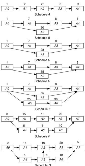
Having established a theoretical foundation of our measures, it is natural to ask how the values of these measures can be used to distinguish between good and bad schedules. Figure 1 shows seven example schedules. Such examples are often used in project management literature to test new tools and techniques [14]. The linear scheduleA consists of five activities on a single source-sink path. So the critical path in

schedule A cannot change. However, even the slightest of delays in any activity will result in a change in the critical value of scheduleA. Therefore, we expect scheduleAto have low flexibility. SchedulesB, C andD consist of the same set of nodes and arcs with exactly the same source-sink paths and so have the same network complexity. However, the durations of activities in these schedules are quite different and hence we expect these schedules to have varying levels of flexibility. Schedule E is obtained by augmenting schedule D with an additional critical path consisting of two new critical activities. This leads to the expectation thatE offers less flexibility compared toD. Finally, scheduleF and Ghave the same set of nodes with G having an additional arc A5−A2. Since this additional arc creates an extra near critical path inG, it would be reasonable to assume thatF has a greater capacity to absorb temporal changes than G.

We now evaluate path shift and value shift for these schedules and show how these measures can be used to determine the flexibility, and hence the quality, of these schedules.

Fig. 1: Example schedules

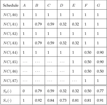
Table 1 lists node centralities and the values of Sp and Sv for the seven schedules of Figure 1. We

observe that, as expected,Sp(A) = 0which is minimum possible, whereasSv(A) = 1which is maximum

possible. These values indicate that although the critical path of scheduleAis absolutely stable (there is only one path), the critical value is extremely unstable as a delay in any activity will directly change the critical value.

TABLE 1: Path shift and value shift of the example schedules (rounded to the nearest hundredth)

Furthermore, despite their identical network topologies, our measures are able to differentiate between the quality of schedules B, C and D based on their flexibility. Since Sp(D) < Sp(C) < Sp(B) and Sv(D) < Sv(C) < Sv(B), our measures indicate that schedule D is the most flexible, while B is the

least. This conclusion is consistent with the scheduling intuition because the non-critical path and the non-critical activities inBare near critical, while this is not the case for scheduleD. As a result we expect B to be more sensitive to changes in activity durations as such changes will affect its critical path and critical value more than scheduleD. We also observe that the flexibility of scheduleC is greater thanB but less than D. Moreover, Sp(D) =Sp(E) while Sv(D)< Sv(E), the former due to the fact that both

schedules have the same non-critical paths while the latter owing to schedule E having more critical activities. Our measures indicate D to be a more flexible schedule which is in line with the scheduling

logic.

Table 1 also shows that both the shift measures assign a lower value to schedule F compared to schedule G. This is in line with the intuitive reasoning that the activities of Gare relatively more near critical and thusGshould be considered less flexible thanF.

The above example cases suggest that a schedule with lower path shift and value shift is more flexible and hence, according to our criterion, of better quality. Therefore, among schedules B−G in Figure 1, D is of the best quality. However, in comparing two schedules, it is possible for one schedule to have a lower path shift while the other has a lower value shift (for example,AandD). In this case, we conclude that the former schedule has a more stable critical path while the latter has a more stable critical value and the overall schedule quality depends on which type of stability is more desirable for a given software project.

4.4 Comparison with the Current Flexibility Measures

The aim of this section is to show that the centrality-based flexibility measures outperform the current metrics of schedule flexibility in discriminating between the flexibility of different schedules. In Section 4.3 we have seen thatSpandSv clearly differentiate between the flexibility of schedulesA−Gin Figure

1. Furthermore, the results obtained are consistent with the scheduling intuition. However, we will see that this is not the case for the existing flexibility metricsf lexseq,RB,dsrpand stab.

The measuref lexseq can give a false impression of flexibility. A schedule with many non-intersecting

parallel paths will have a high value off lexseq even if all the paths are critical, whereas in reality such

a schedule allows no flexibility at all. Furthermore,f lexseq assigns the same value of 2 for the schedules B,C and D as they have the same precedence relations between activities.

The robustness metric RB fails to distinguish between the flexibility of schedules F and G as the additional arc A5−A2 does not change the start and end times of activities, nor does it change the critical value. However, as discussed in Section 3.3, the scheduling logic suggests thatGis less flexible. The two disruption measures dsrp and stabalso have certain drawbacks. Firstly, it is not clear why the two measures respectively use the slacks and one unit delays as increments to calculate schedule disruption. Moreover, it is not clear howdsrp handles critical activities as for these activities bothslack

and numchanges are equal to zero. On the other hand,stabfails to differentiate between schedulesB,C

and D giving a value of 8 for each of these schedules.

In addition to the issues discussed above, none off lexseq,dsrpandstabhas a specific range of values.

5

C

S

1: O

H

C

S

This section discusses an application of our proposed schedule flexibility analysis to the Obesity Health Clinic System (OHCS) implemented for an obesity clinic at Saudi Aramco1 in Dhahran, Saudi Arabia. Within this system, patient and health team member profiles can be created, updated and deleted. The OHCS allows health team members and patients to create obesity reducing goals. The goals are added to the ‘bank of ideas’ and classified under the appropriate category (for example, physical, dietary etc). These goals can also be customized according to individual patient needs by the health team. The OHCS also has the ‘goal suggestion’ feature which helps the health team to find appropriate goals for a patient according to his health condition. Moreover, the OHCS has a report engine that allows health team members to generate reports about patient performance and popular goals.

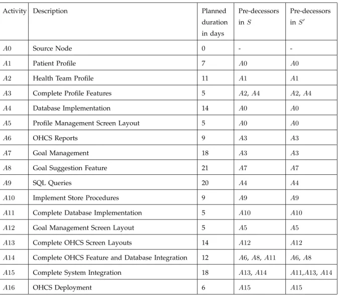
TABLE 2: Activities, durations and predecessors for OHCS implementation schedules

Often the activities of a software development project can be planned in different ways. Thus it is quite possible to come up with alternative schedules to plan the activities of a project. In our first case study, the project team proposed two schedules for the implementation of the OHCS. Generally in such cases, the project team has to base their choice of schedule on their experience and mutual consensus. Here we show that the flexibility analysis developed in this paper can greatly facilitate the project team in making informed decisions in this regard.

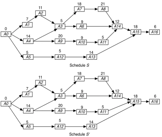
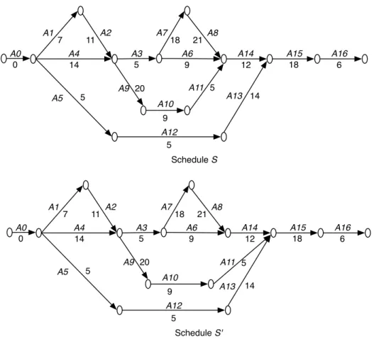
Fig. 2: The proposed OHCS schedules

Table 2 lists the activities of the OHCS project, their planned durations in days and their predecessors in the two schedules designed by the project team. The OHCS project consists of sixteen activities. The business logic of the system is implemented during activitiesA1,A2,A3,A6,A7andA8, while the back-end functionalities are implemented during A4, A9, A10 and A11. Similarly, the OHCS user interface layout is implemented during activities A5, A12 and A13. The activity A14 is performed to carry out the integration of the business logic and the back-end features of the OHCS, whereasA15is performed to complete the integration of the different subsystems of the OHCS. The final project activity A16is to deploy the system. Figure 2 show the CPM networks for the schedulesSandS0 proposed for the OHCS project. Note that A0 is a dummy source node added so that the schedule networks have exactly one source and one sink. This is a standard practice in project management.

5.1 Shift Measures Applied to the OHCS

The CPM approach works by calculating the longest duration path passing through each project activity and uses this information to obtain the critical paths and the critical value of a schedule. These calculations can be carried out by using any standard project management tool such as Microsoft Project. In this study, we use @Risk2 _{which is a project risk management add-in for Microsoft Excel. Our preference for @Risk} is due to its ability to run Monte Carlo simulation readily (see Section 5.2).

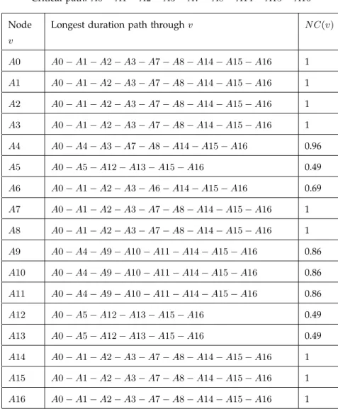
TABLE 3: Flexibility measures for scheduleS

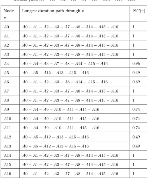
For both the OHCS schedules, the critical value turns out to be 98 days while the critical path is the directed source-sink pathA0−A1−A2−A3−A7−A8−A14−A15−A16. We now use the flexibility measures defined in Section 4.2 to predict and compare the quality of schedules S and S0. Table 3 and Table 4 list the values of node centralities and the shift measures for the schedulesSandS0, respectively. The path shift and the value shift for the schedule S equals 0.71 and 0.86, respectively. Analyzing S0 shows that Sp(S0) = 0.67 < Sp(S) and Sv(S0) = 0.84 < Sv(S). From these results, we expect that the

critical path and the critical value ofS0 _{will remain relatively more stable if some activities are delayed.}

TABLE 4: Flexibility measures for scheduleS0

5.2 Validation Using Monte Carlo Simulation

The predictive analysis performed in Section 5.1 can be validated by running Monte Carlo simulations of the two proposed schedules. Over the years, Monte Carlo simulation has emerged as an important decision support tool in a variety of domains including finance, project management and scheduling [12, 37, 38]. From a scheduling perspective, Monte Carlo simulations enable a decision maker to forecast the likely behavior of a schedule based on the uncertainty in activity durations [12, 38]. The uncertainty in activity duration is encoded by defining a probability distribution for each such activity. For scheduling applications, the triangular distribution is the most popular [37, 38], in which the shortest, longest and expected duration of each vulnerable activity is specified by a domain expert. This is followed by the selection of a suitable sampling method. Thesimple Monte Carlo samplingis the traditional technique for using random or pseudo-random numbers to sample from a probability distribution. These techniques are completely random as any given sample value may fall anywhere within the range of the input

sample space. Typically, a large number of samples are required to match the input distributions. On the other hand, theLatin hypercube sampling [39] divides the input probability distributions into a finite number of equally probable intervals and then chooses a sample randomly from each interval. This type of ‘stratified sampling’ ensures that even with a small number of samples the input distribution is matched very closely [39]. After a sampling method is selected, Monte Carlo simulation generates a probability distribution of the outcome values. In scheduling, we are generally interested in the distribution of critical value [12].

Considering their merits, here we apply a triangular distribution to each input and use Latin hypercube sampling to run Monte Carlo simulations. We select seven activities, namelyA6,A8,A9,A10,A13,A14

and A15 that the project team considered as more susceptible to potential delays and apply triangular distribution to the durations of these activities in order to simulate these potential delays.

We employed @Risk to run the simulations of S and S0 _{by specifying a minimum, mostly likely and} maximum duration for each of the vulnerable activities. The minimum duration was set one day less than the planned duration, whereas the most likely duration was set as the planned duration. On the other hand, the maximum value for the triangular distribution was chosen as double of the planned duration to account for significant delays. While running simulations, we tracked changes in the critical value and the critical path of the schedules.

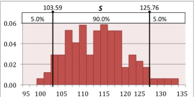
Fig. 3: Change of critical value and critical paths during Monte Carlo simluations of S andS0

Figures 3 (a-b) show the distribution of the critical value for the OHCS schedulesS andS0as generated by @Risk after 100 simulation runs, while Figure 3 (c) describes the stability of critical paths of S and S0 during these simulation runs. Note that 100 iterations suffice due to our choice of Latin hypercube sampling, which requires fewer samples. The minimum, mean and maximum critical value of S are recorded to be 99.36,114.22 and 133.61, respectively. It is noteworthy that the planned critical value of

98 days for the schedule was not achieved in any of the simulation runs. In fact, in only about 10% of the iterations the critical value was less than105. Similarly, the simulation results show that the critical path ofS changed in 55% of the instances, which though not as bad as the variability exhibited by the critical value, is still quite high.

On the other hand, the critical path and the critical value ofS0display relatively greater stability when the same triangular distributions are applied to the activities ofS0. It was observed that the critical path changed in only 43% of the iterations while the critical value was distributed between 97.20and129.85

with an average of114.03. All these findings are in line with the flexibility analysis performed in Section 5.1 and indicate thatS0 _{is a more flexible schedule for the OHCS project.}

5.3 Comparison with the Example Cases

Comparing the results obtained by applying value and path shift to the schedules S and S0, and their validation using Monte Carlo simulations, with the results obtained in Section 4.3 reveals an interesting analogy. Indeed, schedules S and S0 can be compared with the schedules F and G considered among the example cases. Recall that schedulesF andGconsist of the same activities with the same durations. They only differ in one arc. However, even this minor change results in different degrees of flexibility for these schedules as determined by the shift measures. Since F has lower path and value shifts than G, it was concluded in Section 4.3 that F was more flexible. It was remarked that the relative lack of flexibility ofGcould be attributed to it having more near-critical activities (more nodes with large node centralities) thanF.

Analogously, schedules S and S0 _{consist of the same activities having the same durations, with the} only difference being a single arc. The shift measures are once again able to distinguish between the flexibility of these very similar schedules and we conclude thatS0 is more flexible thanS. Here also we can explain the lower flexibility ofS in terms of three of its nodesA9,A10and A11having larger node centralities (see Table 3 and Table 4). Thus the values and interpretation of node centrality, path shift and value shift remain consistent. Moreover, the results of Monte Carlo simulation support our findings.

5.4 Qualitative Analysis of Feedback

In this section, we present qualitative analysis of the feedback received from software engineers and developers, both from academia and industry, on using our schedule flexibility measures in practice. The participants belonged to one or more of the following categories.

• _{OHCS project team members}

• Researchers from the Information and Computer Science Department, King Fahd University Univer-sity of Petroleum and Minerals

• Researchers from the Department of Computer Science, University of Calgary

• Researchers from the Department of Electrical and Computer Engineering, University of Calgary • Industrial practitioners from Saudi Aramco

• Software release planning experts from Microsoft Canada

The participants were either first-hand users of the flexibility analysis presented in this paper as part of the OHCS project team or had been provided full project information and technical details needed to implement our approach in projects of their own. A total of 17 professionals participated in the study.

The qualitative data was collected by conducting interviews with the participants. Their experiences were documented using mainly two open-ended questions, encompassing the advantages and difficulties associated with applying the proposed flexibility measures. The interviews were kicked off with the question: ‘From your observation and experience, what are the characteristics of our flexibility measures

that helps you distinguish a set of project schedules’? We used follow-up questions to clarify and gather more details about the strengths and limitations mentioned by the participants.

The participants indicated four key advantages of the proposed flexibility measures. First, the measures were deemed helpful in predicting the impact of activity delays on critical paths and critical values associated with network-based schedules by a large majority of the participants. Second, there was a consensus that path shift and value shift measures helped in early prediction of how schedules would respond to changes in activity duration. Third, most of the interviewees agreed that the proposed flexibility measures lead to effort saving by pointing out lack of flexibility in a project schedule. Finally, the feedback from the participants also indicated the fixed range between 0 and 1 as a major strength of the new measures as it facilitates in comparing different schedules.

The participants in the study did not indicate any major disadvantages in applying the proposed flexibility measures as they do not require additional computational effort and can be computed alongside the standard CPM calculations. However, two of the participants indicated that the proposed flexibility analysis only accounts for task schedules and does not explicitly consider resource allocation constraints. Similarly, feedback from another participant indicated that the flexibility measures should perhaps be modified to provide some indication of how project team members could be best matched with the project tasks. One participant from construction management background pointed out that our approach could just as well be implemented on construction management and other industrial management projects. We agree with all these participants and have incorporated their suggestions in our plans for future work.

6

C

S

2: L

C

A

S

This section discusses an application of our schedule flexibility analysis to the Life Cycle Assessment (LCA) system implemented for an ecologically sustainable development consulting firm in Dhahran, Saudi Arabia. Within this system, building architecture engineers investigate the existing building prac-tices from the energy and environmental perspectives. The LCA system allows architecture engineers to evaluate the environmental burdens associated with a product, system or activity by quantifying the energy impact of different building materials.

TABLE 5: Activities, durations and flexibility analysis of the LCA implementation scheduleT

Table 5 lists, among other things, the activities of the LCA development project and their planned durations in days designated by the project team. The LCA project consists of thirty four activities. The user profiles are implemented during activities A1 and A2, while the business logic of the system is implemented during the activities A3, . . . , A9. The LCA system user interface layout and database is implemented during activitiesA10and A11, respectively. The environmental impact assessment and

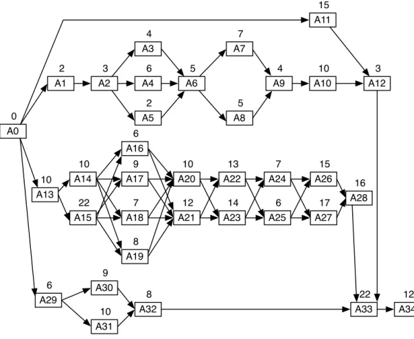
improvement analysis is carried out during activities A13, . . . , A28. Finally, the inventory analysis is implemented duringA29, . . . , A32. ActivityA33is performed to complete the integration of the different subsystems of the LCA system. The final project activityA34is to deploy the system. Figure 4 shows the CPM network schedule for the LCA system project as designed by the project team.

Fig. 4: The LCA scheduleT

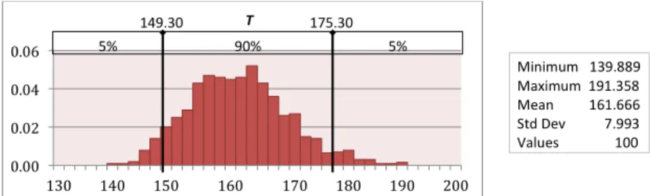
We aim to apply the centrality-based flexibility measures on scheduleTand compare its flexibility with schedules S and S0 of Case Study 1. Like the first case study, we perform the CPM calculations using @Risk. For schedule T the critical value turns out to be 141 days while the critical path is the directed source-sink pathA0−A13−A15−A17−A21−A23−A24−A27−A28−A33−A34. The node centralities and the flexibility measures are computed, as in Section 5, to quantify the flexibility of scheduleT and compare it withS andS0. Table 5 lists the values of node centralities and the shift measures for schedule T. The path shift and the value shift ofT are0.65and0.76, respectively, both of which are lower than the corresponding values for schedules S andS0. These results forecast that, if some activities are delayed, the critical paths and the critical value of T will demonstrate greater stability compared toS andS0.

We validate this predicted behavior by running a Monte Carlo simulation of schedule T. In order to maintain consistency with Case Study 1, we apply triangular distributions to the durations of thirteen activities, namelyA1,A4,A5,A7,A10,A11,A13,A21,A24,A28,A30,A32andA33that were considered most vulnerable to potential delays by the project team. Again, as in the OHCS case study, the minimum duration for the triangular distribution of each activity is set one day less than the planned duration, the most likely duration is set as the planned duration, while the maximum value for the triangular distribution is chosen as double of the planned duration to account for significant delays. Furthermore, we select Latin hypercube sampling to run the Monte Carlo simulation. During simulation runs, we tracked changes in the critical value and the critical path of the LCA scheduleT.

Fig. 5: Change of critical value and critical paths during Monte Carlo simulation runs ofT

Figure 5 (a) shows the distribution of the critical value for scheduleT as generated by @Risk after 100 simulation runs, whereas Figure 5 (b) compares the stability of critical paths of T with those of S and S0 during these iterations. The minimum, mean and maximum critical value ofT turns out to be139.89,

191.36 and 161.67, respectively. We note that the mean critical value of T during simulation runs lies within(161.67−141)/141 = 14.66%of the expected critical value of141. On the other hand, from Figure

3 (a-b), the variation from the expected critical value of98for schedulesS andS0 is respectively16.56%

and16.4%. Thus Monte Carlo simulation results back our prediction that ofS,S0 _{andT, the scheduleT} has a more stable critical value.

The critical path ofT shows even greater stability, remaining unchanged in 71% of the iterations. On the other hand, the critical path ofS is unaltered in45% and that ofS0 remains the same in57% of the iterations. All these findings validate our centrality-based flexibility analysis of schedulesS,S0 and T.

7

D

We have seen that the measures introduced in this paper perform better than the existing measures in distinguishing between the flexibility of different schedules. In this section, we outline some additional characteristics of our approach that make it more attractive for practical use compared to the current techniques for analyzing schedule robustness.

• Ease of Use:Practicability is one of the main criteria for the acceptance of any project analysis technique by the software engineering community. A complex methodology, however effective it may be, is unlikely to attract practitioners as they simply don’t have the time to come to terms with it. The project flexibility analysis presented in this paper has a theoretical foundation in social network analysis, yet it is very easy to implement as suggested by the findings of the qualitative study presented in Section 5.4. The path and value shifts are two numbers ranging between 0 and 1 with a clear interpretation. The simplicity of scale makes it easy to determine the flexibility of schedules. • Computational complexity:Our measures only depend on the basic temporal data of a software project schedule, which is computed as part of the standard CPM calculations. After running the CPM algorithm, the node centralities and the two shift measures can be determined inO(|V|)time, where

|V|is the number of activities in the schedule. Hence, our measures can be evaluated with nominal computational effort. This provides software project managers the ability to measure the flexibility of a schedule alongside CPM calculation and without running complex simulations.

• Scalability: Since our flexibility measures do not require any significant computational effort, they can be easily applied to large-scale software projects. Several centrality-based metrics are routinely applied to complex real-life networks including the World Wide Web, food chains, neuron networks in the brain, ’Facebook’ networks and citation/collaboration networks [40]. Often these networks involve thousands or even millions of nodes and edges. Since path shift and value shift are based on betweenness centrality, they retain their effectiveness irrespective of the size and the complexity of the project schedule. We are planning a large-scale industrial study as part of the future work to demonstrate this feature of our schedule flexibility measures.

• Portability: In this paper, we applied our flexibility analysis to schedules without any time lags between activities. Such time lags are represented as time durations on arcs. It is noteworthy that even in the presence of time lags, equations (2), (3) and (4) remain the same. The only change is that

the duration of a pathpwould be defined asD(p) =P

v∈pD(v) +

P

e∈pl(e), where l(e)is the time

lag on arc e. Furthermore, all the schedules considered in this paper are represented as ‘Activity on Node’ (AoN) networks, i.e., the nodes represent activities while the arcs represent precedence relations between activities. Equivalently, we can adopt the ‘Activity on Arc’ (AoA) formulation by swapping the roles of nodes and arcs. However, path shift and value shift, their scales and interpretations still remain unchanged. To illustrate this fact, let us consider the AoA representations of the OHCS schedulesS andS0.

Fig. 6: ‘Activity on Arc’ representation ofS andS0

Here activities are represented by arcs. As before, let V denote the nodes and E the set of arcs of a schedule network G. For any arc a ∈ E, denote by P(a) the set of source-sink paths that pass through a. Also letD(a)denote the duration of an arc aandD(p) =P

a∈pD(a)be the duration of

a source-sink path p. A critical path is a largest duration source-sink path inG. A critical arc is an arc that lies on a critical path and Enc denotes the set of non-critical arcs inG. To make the shift

measures work in the AoA setting, we just have to make minor changes to formulas (2), (3) and (4). We define thearc centralityof an arca∈E as

AC(a) = maxp∈P(a)D(p)

CV , (5)

where CV denotes, as before, the critical value of the schedule andmaxp∈P(a)D(p)represents the

duration of the longest duration source-sink path in the schedule that passes through a. The value shift and path shift can now be defined as

Sv(G) = P a∈EAC(a) |E| , (6) and Sp(G) = P a∈EncAC(a) |Enc| . (7)

It is easy to see that using these definitions does not change the path durations, the critical paths, the centralities and the values of Sv and Sp. Therefore, the schedule flexibility analysis performed

in this paper is equally applicable to AoN and AoA schedule networks.

8

C

F

W

The present work provides software project managers with a diagnostic technique to estimate the flexibil-ity of a schedule before its implementation. The technique developed in this paper has a strong theoretical background as it is motivated by the concept of betweenness centrality from social network analysis. Additionally, our technique can be applied with minimal computational effort. The two measures, path shift and value shift output two numbers on a scale from 0 to 1 and have a clear interpretation. While

comparing two schedules, the one with lower values of shift measures would perform better when some of its activities are delayed.

We present application of our approach to seven example schedules as well as a real-life software project. The example cases help us understand how the two measures are more useful than the existing flexibility measures, while the results of running Monte Carlo simulation in the case study enable us to verify the predictions made by our measures. We believe that by using the proposed flexibility measures, software project managers will be able to determine the flexibility of a schedule, choose between alternative schedules, recognize some of the risks involved in implementing a schedule and take necessary steps to offset these risks.

For future work, we plan to extend our flexibility measures to resource allocation models [41, 42]. We also plan to conduct a longitudinal industrial study to better understand the role of flexibility measures in predicting the impact of activity delays on the critical paths and the critical value of a schedule. Another direction is to design efficient algorithms for automatic schedule generation. The idea is to generate a schedule satisfying the given task sequencing constraints while minimizing both the path shift and the value shift as much as possible. This would result in a schedule with high degree of flexibility.

The project manager - be it a software development, construction management or an industrial project - plays a critical role in the success or failure of a project [43]. Several key scheduling and planning decisions are subjective and require significant domain expertise and managerial skills. In fact, we feel that the competence of the entire project team affects the project outcome. Thus it seems imperative to consider the ‘human factor’ in the scheduling process. We aim to utilize the competency model concepts presented in [43] to determine how human resources relate to schedule quality.

Recently, Lakhoua [44] employed Object Oriented Project Planning (OOPP) as a tool of analyzing and scheduling industrial systems upgrades and automation. It would be interesting to investigate potential application of our schedule flexibility analysis to industrial systems upgrade projects. Such an application could result in significant savings of time and capital by measuring risk of delays in projects in terms of schedule flexibility.

Another potential area of application is scheduling inventory replenishment. Lin, Wang and Wu [45] have proposed a Forecast Forward Replenishment (FFR) strategy for replenishing vendor-managed in-ventory. The centrality-based schedule assessment techniques introduced in this paper, can potentially be combined with the FFR strategy to produce more robust schedules for inventory management activities.

A

The first author is a Vanier-Banting Scholar (NSERC) and an Izaak-Walton Killam Scholar at the University of Calgary. The second author would like to thank King Fahd University of Petroleum and Minerals, Dhahran, Saudi Arabia for continuous support in research. Both the authors are grateful to the anonymous reviewers for their valuable suggestions that helped in improving the paper significantly.

A0 A1 A2 A3 A4 Schedule A A0 A1 A2 A3 A4 Schedule B 7 8 3 20 A0 A1 A2 A3 A4 Schedule C 7 8 3 28 7 20 8 3 1 1 1 A0 A1 A2 A3 A4 Schedule D 7 8 3 55 1 A0 A1 A2 A3 A4 Schedule E 7 8 3 1 A5 A6 55 25 30 A0 A1 A2 A7 Schedule F 15 10 5 0 A3 20 A4 A5 5 5 A6 10 A0 A1 A2 A7 Schedule G 15 10 5 0 A3 20 A4 A5 5 5 A6 10

A1 A4 A2 11 A3 5 A6 9 A7 18 A8 21 A12 5 A13 14 A5 5 A9 20 A14 12 A11 5 A15 18 A16 6 A10 9 A0 7 14 0 Schedule S A1 A4 A2 11 A3 5 A6 9 A7 18 A8 21 A12 5 A13 14 A5 5 A9 20 A14 12 A11 5 A15 18 A16 6 A10 9 A0 7 14 0 ScheduleS'

    0.00   0.02   0.04   0.06   95   100   105   110   115   120   125   130   135   90.0%   5.0%   5.0%        S   103.59   125.76   Minimum          99.364   Maximum    133.616   Mean                    114.227   Std  Dev                      7.049   Values              100    

(a) Distribution of critical value ofS

  0.00   0.02   0.04   0.06   0.08   0.10   95   100   105   110   115   120   125   130   90.0%   5.0%   5.0%   S'   101.98   126.70   Minimum          97.195   Maximum    129.848   Mean                    114.028   Std  Dev                      7.184   Values              100    

(b) Distribution of critical value ofS0

  45%   55%   57%   43%   40%   45%   50%   55%   60%  

Same  Path   Different  Path  

S   S'  

(c) The change of critical paths ofSandS0

A0 0 A13 10 A1 2 A2 3 A3 4 A11 15 A4 6 A5 2 A6 5 A7 7 A8 5 A9 4 A10 10 A12 3 A14 10 A15 22 A17 9 A20 10 A22 13 A18 7 A16 6 A19 8 A21 12 A23 14 A24 7 A25 6 A26 15 A27 17 A28 16 A29 6 _A30 9 A31 10 A32 8 A33 22 A34 12

      0.00   0.02   0.04   0.06   130   140   150   160   170   180   190   200   90%   5%   5%   T   149.30   175.30   Minimum      139.889   Maximum    191.358   Mean                    161.666   Std  Dev                      7.993   Values              100   0  

(a) Distribution of critical value ofT

  45%   55%   57%   43%   71%   29%   20%   30%   40%   50%   60%   70%   80%  

Same  Path   Different  Path  

S   S'   T  

(b) The change of critical paths ofT compared toSandS0

Schedule S A0 0 A1 7 A4 14 A2 11 A3 5 A9 20 A7 18 A6 9 A8 21 A14 12 A10 9 A11 5 A15 18 A16 6 A5 5 A12 5 A13 14 Schedule S' A0 0 A1 7 A4 14 A2 11 A3 5 A9 20 A7 18 A6 9 A8 21 A14 12 A10 9 A11 5 A15 18 A16 6 A5 5 A12 5 A13 14

TABLE 1: Path shift and value shift of the example schedules (rounded to the nearest hundredth) Schedule A B C D E F G N C(A0) 1 1 1 1 1 1 1 N C(A1) 1 0.79 0.59 0.32 0.32 1 1 N C(A2) 1 1 1 1 1 1 1 N C(A3) 1 0.79 0.59 0.32 0.32 1 1 N C(A4) 1 1 1 1 1 0.50 0.90 N C(A5) · · · 1 0.50 0.90 N C(A6) · · · 1 0.50 0.50 N C(A7) · · · 1 1 Sp(·) 0 0.79 0.59 0.32 0.32 0.50 0.77 Sv(·) 1 0.92 0.84 0.73 0.81 0.81 0.91

TABLE 2: Activities, durations and predecessors for OHCS implementation schedules

Activity Description Planned

duration in days Pre-decessors inS Pre-decessors inS0 A0 Source Node 0 - -A1 Patient Profile 7 A0 A0

A2 Health Team Profile 11 A1 A1

A3 Complete Profile Features 5 A2,A4 A2, A4

A4 Database Implementation 14 A0 A0

A5 Profile Management Screen Layout 5 A0 A0

A6 OHCS Reports 9 A3 A3

A7 Goal Management 18 A3 A3

A8 Goal Suggestion Feature 21 A7 A7

A9 SQL Queries 20 A4 A4

A10 Implement Store Procedures 9 A9 A9

A11 Complete Database Implementation 5 A10 A10

A12 Goal Management Screen Layout 5 A5 A5

A13 Complete OHCS Screen Layouts 14 A12 A12

A14 Complete OHCS Feature and Database Integration 12 A6,A8,A11 A6, A8

A15 Complete System Integration 18 A13,A14 A11,A13,A14

TABLE 3: Flexibility measures for scheduleS

Sp(S) = 0.71,Sv(S) = 0.86, Critical value =CV = 98

Critical path:A0−A1−A2−A3−A7−A8−A14−A15−A16

Node

v

Longest duration path throughv N C(v)

A0 A0−A1−A2−A3−A7−A8−A14−A15−A16 1 A1 A0−A1−A2−A3−A7−A8−A14−A15−A16 1 A2 A0−A1−A2−A3−A7−A8−A14−A15−A16 1 A3 A0−A1−A2−A3−A7−A8−A14−A15−A16 1 A4 A0−A4−A3−A7−A8−A14−A15−A16 0.96 A5 A0−A5−A12−A13−A15−A16 0.49 A6 A0−A1−A2−A3−A6−A14−A15−A16 0.69 A7 A0−A1−A2−A3−A7−A8−A14−A15−A16 1 A8 A0−A1−A2−A3−A7−A8−A14−A15−A16 1 A9 A0−A4−A9−A10−A11−A14−A15−A16 0.86 A10 A0−A4−A9−A10−A11−A14−A15−A16 0.86 A11 A0−A4−A9−A10−A11−A14−A15−A16 0.86 A12 A0−A5−A12−A13−A15−A16 0.49 A13 A0−A5−A12−A13−A15−A16 0.49 A14 A0−A1−A2−A3−A7−A8−A14−A15−A16 1 A15 A0−A1−A2−A3−A7−A8−A14−A15−A16 1 A16 A0−A1−A2−A3−A7−A8−A14−A15−A16 1

TABLE 4: Flexibility measures for scheduleS0

Sp(S) = 0.67,Sv(S) = 0.84, Critical value =CV = 98

Critical path:A0−A1−A2−A3−A7−A8−A14−A15−A16

Node

v

Longest duration path throughv N C(v)

A0 A0−A1−A2−A3−A7−A8−A14−A15−A16 1 A1 A0−A1−A2−A3−A7−A8−A14−A15−A16 1 A2 A0−A1−A2−A3−A7−A8−A14−A15−A16 1 A3 A0−A1−A2−A3−A7−A8−A14−A15−A16 1 A4 A0−A4−A3−A7−A8−A14−A15−A16 0.96 A5 A0−A5−A12−A13−A15−A16 0.49 A6 A0−A1−A2−A3−A6−A14−A15−A16 0.69 A7 A0−A1−A2−A3−A7−A8−A14−A15−A16 1 A8 A0−A1−A2−A3−A7−A8−A14−A15−A16 1 A9 A0−A4−A9−A10−A11−A15−A16 0.74 A10 A0−A4−A9−A10−A11−A15−A16 0.74 A11 A0−A4−A9−A10−A11−A15−A16 0.74 A12 A0−A5−A12−A13−A15−A16 0.49 A13 A0−A5−A12−A13−A15−A16 0.49 A14 A0−A1−A2−A3−A7−A8−A14−A15−A16 1 A15 A0−A1−A2−A3−A7−A8−A14−A15−A16 1 A16 A0−A1−A2−A3−A7−A8−A14−A15−A16 1

TABLE 5: Activities, durations and flexibility analysis of the LCA implementation schedule T

Sp(T) = 0.65,Sv(T) = 0.76, Critical value =CV = 141

Critical path:A0−A13−A15−A17−A21−A23−A24−A27−A28−A33−A34

Activity Description Planned

duration in days Node centrality A0 Source Node 0 1 A1 User Profile 2 0.52 A2 Architect Profile 3 0.52

A3 Import ‘SimaPro’ Style Data Files 4 0.51

A4 Import Excel Style Data Files 6 0.52

A5 Import ‘openLCA’ Style Data Files 2 0.50

A6 File Type Conversions 5 0.52

A7 Create Life Cycle Assessment Flows 7 0.52

A8 Define Life Cycle Assessment Processes 5 0.51

A9 Complete Life Cycle Assessment Work Flows 4 0.52

A10 LCA Screen Layouts 10 0.52

A11 LCA Database Implementation 15 0.38

A12 LCA Business Logic and Database Integration 3 0.52

A13 Import LCA Standard Methods 10 1

A14 Sequential Inventory Calculation Feature 10 0.91

A15 Uncertainty Calculation Feature 22 1

A16 Characterization Feature 6 0.98

A17 Environmental Damage Assessment Feature 9 1

A18 Normalization Feature 7 0.90

A19 Energy Modeling Assessment Feature 8 0.99

A20 Group Analysis 10 0.99

A21 Standard Analysis 12 1

A22 Graphics Based Analysis 13 0.99

A23 Spread Sheet Based Analysis 14 1

A24 Export ‘SimaPro’ Analysis Form 7 1

A25 Export ’openLCA’ Analysis Form 6 0.99

A26 Export Excel Analysis Form 15 0.99

A27 Export Text Analysis Form 17 1

A28 LCA Forms Integration 16 1

A29 Important Construction Products 6 0.41

A30 Compare Construction Materials Method 9 0.40

A31 Compare Construction Products Method 10 0.41

A32 Create New Construction Standard Projects 8 0.41

A33 Complete System Integration 22 1