Bayesian classifiers based on kernel density estimation: Flexible classifiers

(1)

Bayesian classiﬁers based on kernel density estimation: Flexible classiﬁers

Aritz Pérez

*

, Pedro Larrañaga, Iñaki Inza

Intelligent Systems Group, Department of Computer Science and Artiﬁcial Intelligence, University of The Basque Country, Spain

a r t i c l e

i n f o

Article history:

Received 17 September 2007

Received in revised form 16 August 2008 Accepted 22 August 2008

Available online 13 September 2008

Keywords: Bayesian network Kernel density estimation Supervised classiﬁcation Flexible naive Bayes

a b s t r a c t

When learning Bayesian network based classifiers continuous variables are usually han-dled by discretization, or assumed that they follow a Gaussian distribution. This work introduces thekernel based Bayesian networkparadigm for supervised classification. This paradigm is a Bayesian network which estimates the true density of the continuous vari-ables using kernels. Besides, tree-augmented naive Bayes,k-dependence Bayesian classifier and complete graph classifier are adapted to the novelkernel based Bayesian network par-adigm. Moreover, the strong consistency properties of the presented classifiers are proved and an estimator of the mutual information based on kernels is presented. The classifiers presented in this work can be seen as the natural extension of theflexible naive Bayes

classiﬁerproposed by John and Langley [G.H. John, P. Langley, Estimating continuous

distributions in Bayesian classiﬁers, in: Proceedings of the 11th Conference on Uncertainty in Artiﬁcial Intelligence, 1995, pp. 338–345], breaking with its strong independence assumption.

Flexible tree-augmented naive Bayesseems to have superior behavior for supervised

clas-sification among the flexible classifiers. Besides, flexible classifiers presented have obtained competitive errors compared with the state-of-the-art classifiers.

1. Introduction

Supervised classification [6,26] is an outstanding task in data analysis and pattern recognition. It requires the construction of a classifier, that is, a function that assigns a class label to instances described by a set of variables. There are numerous classifier paradigms, among whichBayesian networks(BN)[60,65], based onprobabilistic graphical models (PGMs)[10,50], are well known and very effective in domains with uncertainty. A Bayesian network is a directed acyclic graph of nodes representing variables, and arcs representing conditional independence relations between triplets of sets of variables. This kind of PGM assumes that each random variable follows a conditional probability distribution given a spe-cific value of its parent variables. BNs are used to encode a factorization of the joint distribution among the domain variables, based on the conditional independencies represented by the directed graph structure. This fact, combined with the Bayes rule, can be used for classification.

In order to induce a classiﬁer from data, two types of variables are considered: the class variable orclass C, and the rest of the variables orpredictorsX¼ ðX1;. . .;Xd;Xdþ1;. . .;Xd0Þ.fX₁;. . .;X_dgis the set of continuous predictors andfX_dþ₁;. . .;X_d0gis the set of discrete predictors. Assuming a symmetric loss function, the process of classifying an instancexconsists of choos-ing the classc_{with the highest}_{a posteriori}_probability,_c_¼_arg

cmaxpðcjxÞ. This entails the use of the winner-takes-all rule. Thea posterioridistribution can be obtained in the following way with the BNs:

*Corresponding author. Tel.: +34 943018070; fax: +34 943015590.

E-mail addresses:[email protected](A. Pérez),[email protected](P. Larrañaga),[email protected](I. Inza). Contents lists available atScienceDirect

International Journal of Approximate Reasoning

j o u r n a l h o m e p a g e : w w w . e l s e v i e r . c o m / l o c a t e / i j a r

(2)

pðcjxÞ /

q

ðc;xÞ ¼pðcÞfðxjcÞ ¼pðcÞY d i¼1 fðxijpaiÞ Yd0 j¼dþ1 pðxjjpajÞ ð1Þ

wherepaiis an instantiation of the predictorspai, which is the set of parents ofXiin the graph,pðÞis a probability

distri-bution,fðÞis a density function and

q

ðÞa generalized probability function[17]. This kind of classifier is known asgenerative, and it forms the most common approach in the BN literature for classification[11,25,30,47,48,56,64,73]. Generative classi-fiers use the joint probability function of the predictor variables and the class,

q

ðc;xÞ. They classify a new instance by using the Bayes rule in order to compute the posterior probability,pðcjxÞof the class variable given the values of the predictors (see Eq.(1)). On the other hand,discriminativeclassiﬁers[35,40,70,74]directly model the posterior probability of the class con-ditioned on the predictor variablespðcjxÞ. This work presents a set of generative classiﬁers based on a new family of BNs that we callkernel based Bayesian network.

It has to be highlighted that this work is centered on the difﬁculties of modeling continuous variables directly (without discretization), and their relations in BN paradigm. The modeling of the mixed domains in BNs can be done as follows: to learn a density function conditioned on a discrete variable is equivalent to creating the partitions in the database inducted by the different values of the discrete variable, and then learn the density functions associated with each value of the discrete variable uniquely from the cases of its corresponding partition. In order to improve the readability and simplicity of the pa-per, from here on, we deal with continuous domains only (without discrete predictors).

One of the simplest classiﬁers based on BNs is thenaive Bayes(NB)[25,48,56]. NB assumes that the predictors are con-ditionally independent given the class.Fig. 1a represents an NB structure. In spite of this strong assumption, its performance is surprisingly good, even in databases which do not hold with the independence assumption[23].

The good performance of the NB classifier has motivated the investigation of classifiers based on BNs which relax this strong independence assumption. A set of examples of different structures which break the conditional independence assumption are shown inFig. 1b–d. They are ordered by their structure complexity, which is related with the number of dependencies between variables that they capture. Thus, the complexity ranges from the simplest naive Bayes to the com-plete graph (CG) structure. On one hand, NB structure forbids any arc between predictor variables. On the other hand, the CG structure includes all the possible arcs between predictors. NB does not model any class conditional dependence between predictors, while CG models all the conditional dependencies. In tree-augmented naive Bayes (TAN) structures the maximum number of parents for a predictor is constrained to one plus the class variable and ink-dependency Bayesian classifier (kDB) structures tokplus the class variable. It must be noted that all the structures shown inFig. 1are constrained to graphs with the class variable as the root. The class variable is the father of all predictor variables included in the model (NB augmented classifiers).

The structures themselves represent domain knowledge and can be interpreted in terms of conditional independencies, constructing the associated independence graph. In addition, they represent a factorization of the joint distribution

q

ðc;xÞ, which is based on the relations of conditional (in)dependencies that are inferred from the structure. In most cases the struc-tures and their corresponding factorizations can allow a representation of the joint distribution with fewer parameters. For example, given a domain withrclass labels andddiscrete predictorsXiwithristates, a complete graph structure requires HðrQdi¼1riÞparameters.1On the other hand, a naive Bayes structure requiresHðPdi¼1rriÞparameters.

A classiﬁer based on BNs is determined by the structure of the graph and the distributions and density functions which model the (in)dependence relations between the variables. In order to model a density function of a continuous variable, three approaches are generally considered:

(1) To discretize it and estimate the probability distribution of the discretized variable by means of a multinomial prob-ability distribution.

(2) To directly estimate the density function in a parametric way using, for example, Gaussian densities.

(3) To directly estimate the density function in a non-parametric way using, for example, the kernel density functions [77].

(4) To directly estimate the density in a semi-parametric way using, for example, ﬁnite mixture models[28]. C X1 X2 X3 X4 C X1 X2 X3 X4 C X1 X2 X3 X4 C X1 X2 X3 X4

Fig. 1.Different structure complexities of BN based classiﬁers.

1

(3)

The most widely used approach in the literature on supervised classification is the estimation using the multinomial dis-tribution over the discretized variables. The BN which assumes that all variables follow a multinomial probability distribu-tion is known as Bayesian multinomial network[10,65] (BMN) . This paradigm only handles discrete variables and if a continuous variable is present, it must be discretized with the consequent loss of information[82]. The loss of information is illustrated in Section5.1.1using six continuous artificial domains. In spite of that, using discretization plus multinomial option, the true density is generally estimated with enough accuracy for classification purposes[11]. This approach could have some problems when modeling a graph with a complex structure and/or with variables discretized in many intervals because the number of parameters to be estimated can be very high, e.g.HðrQd

i¼1riÞfor CG. Besides, as the number of

param-eters to be estimated increases, so does the risk of overfitting. Moreover, the number of relevant cases used to compute each parameter can be very low and, therefore, the statistics obtained might not be robust[38]. A battery of BMN-based classifier induction algorithms of different structural complexities has been proposed in the literature: naive Bayes (NB)[25,48,56], tree-augmented naive Bayes (TAN)[30],k-dependence Bayesian classifier (kDB)[73], semi naive Bayes[47,64], Bayesian net-work-augmented naive Bayes[11]and general Bayesian network[11]. From here on, the classifiers which are based on BMN paradigm will be calledmultinomial classifiers.

The second approach directly estimates the true density of the variables using a parametric density. The Gaussian func-tion is the most popular proposal and it usually provides a reasonable approximafunc-tion to many real-world densities[41]. This choice assumes that continuous variables conditioned on a value of their parents follow a conditional Gaussian den-sity. The paradigm, based on BN which makes this assumption, is known asconditional Gaussian network(CGN)[7,32,50– 52,62]. In this work, we reference the classifiers based on CGN asGaussian classifiers. It must be noted that CGNs have fewer complexity difficulties to model complex graphs than BMNs have, e.g. a complete graph with the class and contin-uous predictors needs onlyHðrd2Þparameters to be modeled in the CGN paradigm. Besides, the estimation of the param-eters is more reliable because they are learned from the partitions induced only by the class (by averagen=rcases, where nis the number of cases in the training set). If the true densities are not too far from the Gaussian, the classifiers based on CGNs obtain classification error rates at least equal to the classifiers based on BMNs[62]. Although a Gaussian density may provide a reasonable approximation to many real-world distributions, it is certainly not always the best approxima-tion, e.g., bimodal densities. The decrease of the classification performance due to the loss of information under the Gaus-sian assumption is illustrated in Section 5.1.1. This suggests another direction in which we might profitably extend and improve the Gaussian (parametric) approach: by using more general approaches to density estimation, e.g., kernel density estimation[41](non-parametric).

In order to break with the strong parametric assumption, this work presents the kernel based Bayesian network (KBN) paradigm. The KBN paradigm uses the non-parametrickernel density estimationfor modeling the conditional density of a continuous variable given a specific value of its parents,fðxjC¼cÞ. The kernel estimation method can approximate more complex distributions than the Gaussian parametric approach. Moreover, kernel density estimation can be seen as a more flexible2_{estimator compared to the multinomial distribution, in the same way that kernel density estimation is considered} more flexible than the histograms[77].

The alternative for breaking with the strong parametric assumption is the semi-parametric approach. The semi-paramet-ric estimation combines the advantages of both parametsemi-paramet-ric and non-parametsemi-paramet-ric estimators. This approach is not restsemi-paramet-ricted to speciﬁc functional forms, and the size of the model only grows with the complexity of the problem being solved[4]. On the other hand, the process of learning the semi-parametric model using the data set is computationally intensive compared to the simple procedures needed for parametric or non-parametric learning procedures[4]. One of the most commonly used non-parametric approaches is the so-called mixture model[28,55]and, especially, Gaussian mixture model[5,55]. However, this work is focused in the non-parametric kernel based approach.

This work is an introduction of the KBN paradigm limited to the supervised classification using the Bayes rule. Conse-quently, we present the KBN paradigm and a battery of classifier induction algorithms supported by it, many of them adapted from the algorithms developed for the Bayesian multinomial network paradigm (NB [25,48,56], TAN [30] and kDB[73]). The classifiers presented are ordered by their structural complexity, ranging from naive Bayes to complete graph. We call the classifiers based on the KBN paradigmflexible classifiers. The origin of the term flexible comes from flexible naive Bayes classifier[41], i.e. the NB structure in the KBN framework.

It must be noted that the BMN, CGN and KBN paradigms handle discrete variables similarly. Thus, given a discrete domain (with discrete predictors only) and a structure, the three paradigms represent the same factorization of the joint distribution. The experimentation of this work has been performed in continuous domains for highlighting the differences between the BMN, CGN and KBN paradigms.

The paper is organized as follows. Section2introduces the non-parametric kernel based density estimation which will be used to learn the KBN based classifiers. Section3presents a group of novel estimators for the computation of the amount of mutual information based on kernels. Their corresponding expressions will be used by the classifier induction algorithms proposed. Section4introduces a set of classifier induction algorithms, based on KBN. They are ordered by their structural complexity: flexible naive Bayes, flexible tree-augmented Bayesian classifier, flexible k-dependence Bayesian classifier

2

We use theﬂexibilityterm in a qualitative way, not as a quantitative measure. It represents the capability of modeling densities of different shapes with precision. For example, kernel density estimation is more ﬂexible than the Gaussian approach because it can model clearly better densities with more than one mode (see Section5.1.1).

(4)

and flexible complete graph classifier. Note that except for flexible naive Bayes[41], the rest of these classifiers are novel approaches. The computational and storage requirements of the proposed algorithms are also analyzed. Moreover, the desir-able asymptotic property of the flexible classifiers (strong pointwise consistency[41]) is proved. In Section5the experimen-tal results for the classifiers proposed are presented and analyzed. The experimenexperimen-tal study includes results in ten kinds of artificial datasets and 21 datasets of the UCI repository[59]. The artificial domains illustrate the advantages of the classifiers based on KBN paradigm, which model the correlations between predictors, for handling continuous predictor variables. They also illustrate the loss of information due to the discretization process and the effect of the smoothing degree in the classi-fication performance. The classiclassi-fication error in the 21 UCI repository datasets is estimated for the presented algorithms and for 10 benchmarks. The estimated errors are compared using the Friedman plus Nemenyi post hoc test[19]. Additionally, the effect of the smoothing degree in classification performance is studied in the selected datasets. The estimation of the bias plus variance decomposition of the expected error[46]is also performed in some of the selected UCI data sets. And finally, Section6summarizes the main conclusions of our paper and exposes the future work related with the KBN paradigm for classification.

2. Kernel density estimation

The kernel basedd-dimensional estimator[80]in its more general form is fðx;HÞ ¼n1X

n

i¼1

KHðxxðiÞÞ ð2Þ

whereHis addbandwidth or smoothing matrix (BM),x¼ ðx1;. . .;xdÞis ad-dimensional instantiation ofX,nis the number

of cases from which the estimator is learned,iis the index of a case in the training set, andKHðÞis the kernel function used.

Note thatXis a multivariate variable and, thus,fðx;HÞis a multivariate function. The kernel based density estimatefð;HÞis determined by averagingnkernel densitiesKHðÞplaced at each observationxðiÞ. The kernel functionKHðÞused is deﬁned as:

KHðxÞ ¼ jHj1=2KðH1=2xÞ ð3Þ

assuming thatKis ad-dimensional density function. A kernel density estimator is characterized by means of (1) The kernel densityKselected.

(2) The bandwidth matrixH.

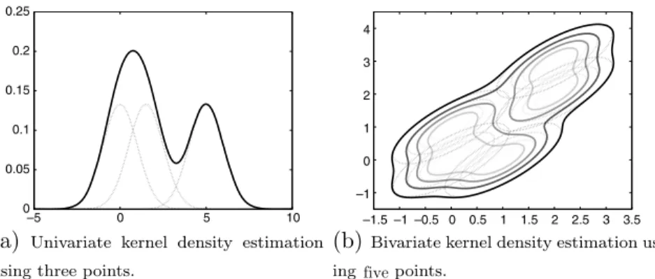
Hplays the role of scaling factor which determines the spread of the kernel at each coordinate direction. The kernel den-sity estimate is constructed centering a scaled kernel at each observation. So, the kernel denden-sity estimator is a sum of bumps placed at the observations. The kernel functionKðÞdetermines the shape of the bumps. The value of the kernel estimate at the pointxis simply the average of thenkernels at that point. One can think of the kernel as spreading a ‘‘probability mass” of size 1=nassociated with each data point in its neighbourhood. Combining contributions from each data point means that in regions where there are many observations it is expected that the true density has a relatively large value. The choice of the shape of the kernel function is not particularly important. However, the choice of the value for the bandwidth matrix is very important for density estimation[80]. Examples for the univariate and bivariate density estimation are shown inFig. 2a and b. Our KBN paradigm uses thed-dimensional Gaussian density with identity covariance matrix,R¼I, in order to esti-mate density functions:

KðxÞ ¼ ð2

pÞ

d=2_exp ð1=2xT_x_Þ_N_ð_0;_I_Þ _ð₄_Þ –5 0 5 10 0 0.05 0.1 0.15 0.2 0.25 –1.5 –1 –0.5 0 0.5 1 1.5 2 2.5 3 3.5 –1 0 1 2 3 4

Fig. 2.Univariate and bivariate Gaussian kernel density estimators. Broken and solid lines represent the contribution of each kernel to the density

(5)

It must be noted that one can use another kernel function as well, such as Epanechnikov, biweight, triweight, triangular, rect-angular or uniform[77,80].

Thus,KHðxxðiÞÞis equivalent toNðxðiÞ;HÞdensity function.His a square symmetric matrixdd, and it has, in its most

general form,dðdþ1Þ

2 different parameters. This number of parameters can be very high, even for low dimensional densities. This suggests constrainingHto a less general form. For example, if a diagonal matrix is used, onlyddifferent parameters must be learned.

2.1. Selecting the bandwidth matrixH

The selection of a good BMHis crucial for the density estimation, even more than the kernel generic functionKðÞ[18].H establishes the degree of smoothing of the density function estimation.

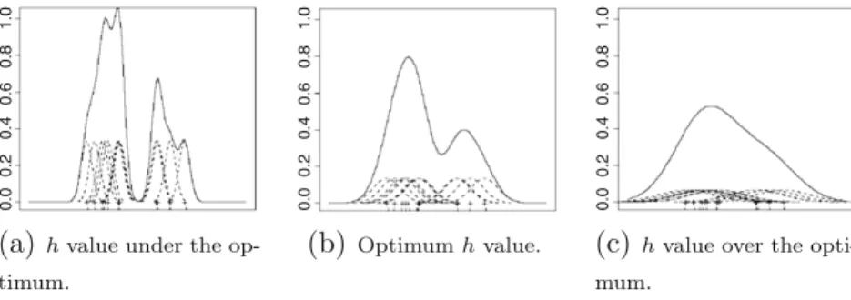
In the univariate case, the smoothing degree depends on a unique parameter,h.Fig. 3shows the effect of the parameterh in the estimation of the true density using the same twelve training cases. Intuitively, withhnear to zero, a noisy estimation is obtained by theundersmootheffect (seeFig. 3a). Ashincreases the noise in the estimation is reduced and the univariate density begins to approximate the true density, until the optimum3_{is reached (see}_{Fig. 3b). As}_h_{increases, and distances itself} from the optimum, the estimation starts to lose details due to theoversmootheffect (seeFig. 3c). Finally, ashtends to1, the function becomes uniform.

The degree of smoothing is crucial for density estimation[80], e.g. for minimizing the mean squared error. On the other hand, the influence of the smoothing degree does not have such a crucial role in classification problems under 0–1 loss func-tions, since density estimation is only an intermediate step for classifying. For example, Gaussian approach obtains good re-sults in many non-Gaussian domains[62]. Intuitively, smoothing degree controls the sensitivity of the classifier to changes in the training set. When the smoothing degree tends to zero, flexible complete graph classifier tends to the nearest neighbor classifier (maximum sensitivity). When the smoothing degree tends to infinity, it tends to the Euclidean distance classifier (minimum sensitivity)[68]. The effect of the smoothing degree in supervised classification has been empirically studied in Sections5.1.2 and 5.2.3.

In order to guarantee an efﬁcient parametrization of a great number of densities, our goal is to use a computationally inexpensive technique to compute the BMH. The number of parameters to be estimated for the speciﬁcation of a full band-width matrix for ad-dimensional density isdðdþ1Þ=2. This number becomes unmanageable very quickly asdincreases, which suggests thatHshould be restricted to a simpler form[78]. In this work we usedifferential scaled[78]approach be-cause it depends on a unique smoothing parameterh:H¼diagðh2₁;. . .;h2_dÞ ¼h2diagðs2

1;. . .;s2dÞ, wherehi is the smoothing

parameter of the variableXi;siis a dispersion measure (e.g. sample standard deviation ofXi) anddiagðÞrepresents a diagonal

matrix. This parametrization allows different amounts of smoothing in each coordinate direction and it performs an implicit standardization of the variables.

The principal problem selecting optimum BM, in the majority of practical situations, is that the real density function is unknown. Thus, in general, it is impossible to optimize any appropriate loss criteria (a distance function between the real and estimated densities). In our work, we use thenormal rule[77]. It selects the BM that minimizes themean integrated square errorof the estimated density, under the assumption that the variables follow a multidimensional Gaussian density with identity covariance matrixI. Under this assumption we can compute the optimumhas follows[77]:

h¼ 4

ðmþ2Þn

1

mþ4

ð5Þ

wheremis the number of continuous variables in the density function to be estimated in spite of the number of continuous variables in the domain,d. For example, in order to model the densityfðx1;. . .;xlÞwe setm¼lin Eq.(5).

We have chosen the normal rule plus differential scaled[78]approach because it obtains density estimations that are good enough for classifying (see Sections5.1.2 and 5.2.3). Furthermore, we know that the normal rule tends to oversmooth

0.0 0.2 0.4 0.6 0.8 1.0 0.0 0.2 0.4 0.6 0.8 1.0 0.0 0.2 0.4 0.6 0.8 1.0

Fig. 3.The effect in the density estimation of different smoothing degrees, controlled by the parameterh.

3

The optimum is defined in terms of a loss function. Mean squared error and classification error are usually used in density estimation and classification, respectively. The optimum term is defined as the parameter value which minimizes the selected loss function.

(6)

[80]the estimation and, thus, it could obtain more stable estimations with noisy data, i.e. estimations with less variance. At the same time, it avoids the increase of the high computational requirements related to the classifier learning process (seeTable 1). It only has to compute a fixed number of operations independently from the dimension of the density and the number of examples used to estimate it. There are other approaches to decide the smoothing degree for obtaining a good classification performance. The wrapper approach[43,45]could be one of the most interesting procedures from the perfor-mance point of view (see Sections5.1.2 and 5.2.3). But it involves intensive computations with flexible classifiers, especially compared with the normal rule.

3. Mutual information and conditioned mutual information estimators

In this section we propose a set of novel estimators based on kernels for the computation of the amount of mutual and conditioned mutual information[15]. These estimators will be used in the classiﬁer induction algorithms presented in Sec-tion4. The estimators are presented in their multivariate form and they inherit the ﬂexibility properties of the kernel density estimation. Thus, we think that they are suitable to compute the amount of mutual information between any pair of contin-uous variables.

Some mutual information based measures are directly related to the expected error of BN based classiﬁers at different structural complexity levels[61]. Improving the conditioned mutual information,IðXi;XjjCÞ, is likely to decrease the Kullback

Leibler divergence between the true and the estimated joint probability distribution. The algorithm TAN proposed by Fried-man et al.[30], which guides the structural learning with the conditioned mutual information, ﬁnds a maximum likelihood TAN structure. Besides, the rank of variables obtained with the use of mutual information,IðXi;CÞ, sorts the variables by the

class entropy reduction,HðCjXiÞ. The class entropy reduction is directly related with the discriminative power of a variable

[61]. For example, ifIðXi;CÞ>IðXj;CÞthenHðCjXiÞ<HðCjXjÞand, therefore, the classiﬁer which includes only the variableXi

instead ofXjtends to obtain lower classiﬁcation errors.

The amount of mutual information between two multivariate variables (random vectors)XandYis deﬁned as[15] IðX;YÞ ¼ Z fðx;yÞlog fðx;yÞ fðxÞfðyÞdxdy¼Epðx;xÞ log fðx;yÞ fðxÞfðyÞ ð6Þ

Based on this deﬁnition we propose the following estimator,bIðX;YÞ, for the amount of mutual information between two con-tinuous multivariate variables X and Y, IðX;YÞ, using kernel density estimation based on a training set of size n;fðxð1Þ_;_yð1Þ_Þ_;_{. . .}_;_ð_xðnÞ_;_yðnÞ_Þg_: bIðX;YÞ ¼1 n Xn i¼1 log ^_f_ð_xðiÞ_;_yðiÞ_Þ ^_f_ð_xðiÞ_Þ_f^_ð_yðiÞ_Þ ð7Þ

where^fðÞis a kernel based density estimation (see Eq.(2)). Note that Eq.(7)estimates the expectance of the function log½fðx;yÞ=ðfðxÞfðyÞÞ, when the instances of the training set are independent and identically distributed[6]. This estimation becomes exact in the limit, asn! 1[6]. Another proposal based on kernels can be found in[57].

Alternatively, in order to compute the amount of mutual information between a multivariate continuous variableXand a multivariate discrete variableCwe propose the following estimator:

bIðX;CÞ ¼1 n Xn i¼1 log

q

^ðx ðiÞ_;_cðiÞ_Þ ^_f_ð_xðiÞ_Þ_^_p_ð_cðiÞ_Þ¼ 1 n Xn i¼1 log ^_f_ð_xðiÞ_j_cðiÞ_Þ ^ fðxðiÞ_Þ ð8Þ

where

q

^ðxðiÞ_;_cðiÞ_{Þ ¼}_^_p_ð_cðiÞ_Þ^_f_ð_xðiÞ_j_cðiÞ_Þ_._^_p_ð_c_Þ_{is the estimated multinomial distribution of variable}_C_and^_f_ð_x_j_c_Þ_{is the kernel based}

den-sity estimator of variableXconditioned onC¼c(computed with the partition of the cases which have the class valueC¼c). The amount of mutual information between two multivariate continuous variables,XandY, conditioned on a multidi-mensional multinomial variableCis deﬁned as

IðX;YjCÞ ¼X jCj c¼1 pðcÞIcðX;YÞ ð9Þ whereIcðX;YÞ ¼Epðx;xjC¼CÞ logfðxfðjcxÞf;yjðcyÞjcÞ

. Using Eqs.(7) and (9), we propose the following estimator for the amount of condi-tioned mutual information:

Table 1

Storage and computational requirements of a classiﬁer with a kDB structure based on both KBN paradigm, with the differential scaled bandwidth matrix plus the normal rule approach, and CGN paradigm

CGN based KBN based

Training space Testing time Training space Testing time

Hðrd2Þ Hðrdðkþ1ÞÞ Hðndþrðdþ1ÞÞ Hðndðkþ1ÞÞ

The domain hasdpredictor variables andrclasses, the training set hasncases. The computational requirements have been obtained for classifying a new instance.

(7)

bIðX;YjCÞ ¼X jCj c¼1 ^ pðcÞ1 nc Xc:nc i¼c:1 log ^ fðxðiÞ_;_yðiÞ_j_c_Þ ^ fðxðiÞ_j_c_Þ^_f_ð_yðiÞ_j_c_Þ ð10Þ

The super-indexc:jrefers to thejth case in the partition induced by the valuec, andncis the number of cases verifying that

C¼c.

All the estimators presented in Eqs.(7), (8) and (10)can be adjusted to any KBN based classiﬁer becauseX,YandCcan be of any arbitrary dimension.

4. Classifiers based on kernel based Bayesian networks: flexible classifiers

The densities to be estimated in the KBN paradigm with continuous predictors are of the formfðxjy;cÞ,XandYbeing con-tinuous multivariate predictor variables andCthe class variable, a univariate discrete variable. That is the essence of the KBN paradigm. The estimation of the density functionfðxjy;cÞcan be determined in the following form using kernel density estimation: fðxjy;cÞ ’^fðxjy;cÞ ¼ ^ fðx;yjcÞ ^ fðyjcÞ

As we have explained at the beginning of Section1, in order to classify a new unlabeled instance,x, the factorization of

q

ðc;xÞ is evaluated for every value of the class,c2 f1;. . .;rg. Then the a posteriori probabilities for each class,pðcjxÞ, are obtained using the Bayes rule. Finally, classiﬁcation is performed under winner-takes-all rule, i.e. choosing the classc_{with the}

max-imum a posteriori probability,c_¼_arg

cmaxpðcjxÞ. Note that in the classiﬁcation of an unlabeled case all the instances in the

training set are used for computing the factorization based on kernel density estimation (see Section2).

Typically, for modeling domains with continuous and discrete variables CGN paradigm has the following structural con-straint: a continuous predictor cannot be parent of a discrete predictor. This constraint could be avoided for the KBN para-digm (and also for the CGN) using the Bayes rule as follows:

pðxdjxc;cÞ ¼pðxd;cÞpðxcjxd;cÞ=pðcÞpðxcjcÞ

whereXdis a multivariate discrete variable (discrete random vector) andXca multivariate continuous one. However, as we

have noted before, this work is centered on the difﬁculties of modeling continuous variables and their relations in the KBN paradigm.

The following sections present a group of flexible classifier induction algorithms, ordered by their structural complexity: flexible naive Bayes, flexible tree-augmented naive Bayes, flexible k-dependence Bayesian classifier and complete graph Bayesian classifier. Note that all the classifiers presented in this paper are extensions of the flexible naive Bayes classifier [41]. Thus, in the presented models, the class variable is the father of each predictor variable. Examples of their different structure complexities are shown inFig. 1.

4.1. Flexible naive Bayes

The least complex structure is the naive Bayes structure (NB structure), which assumes that predictor variables are con-ditionally independent given the class. Thenaive Bayesclassifier induction algorithm (NB)[25,48,56]learns the complete na-ive Bayes structure, which is knowna priori. The accuracy obtained with this classifier is surprisingly high in some domains, even in datasets that do not obey its strong conditional independence assumption[23]. Thanks to the conditional indepen-dence assumption, the factorization of the joint probability is greatly simplified.

Originally, NB classifier was introduced for the BMN (multinomial NB or mNB) and it was adapted to the KBN paradigm (flexible NB or fNB) by John and Langley[41]. This classifier has been recently used in[8,53,54]. It must be noted that our version of the fNB uses the normal rule[77]for computinghinstead of the heuristic proposed in[41].

4.2. Flexible tree-augmented naive Bayes

The tree-augmented naive Bayes structures (TAN structures) break with the strong independence assumption made by NB structures, allowing probabilistic dependencies among predictors. The TAN structures consist of graphs with arcs from the class variable to all the predictors, and with arcs between predictors, taking into account that the maximum number of parents of a variable is one plus class. Example of the TAN structure is shown inFig. 1b.

This section introduces the novel adaptation of Friedman et al.’s[30]algorithm to the KBN paradigm. Friedman et al.’s algorithm[30]follows the general outline of Chow and Liu’s procedure[13], but instead of using the mutual information between two variables, it uses conditional mutual information between predictors given the class variable to construct the maximal weighted spanning tree. In order to adapt this algorithm to continuous variables, we need to estimate the mu-tual information between every pair of continuous predictor variables conditioned by the class variableIðXi;XjjCÞ, computing

(8)

The algorithm[30]starts from a complete NB structure and continues adding allowed edges between predictor until the complete TAN structure is formed. The edges are included in the order of decreasing estimation of the conditional mutual information,IðXi;XjjCÞ. The edges included between predictors create a tree structure. In order to decide the direction of

the edges, we randomly select one predictor as the root of the tree and transform the edges between predictors into arcs. Originally, the TAN algorithm was introduced for BMN (multinomial TAN of mTAN)[30]. This paper adapts it to the novel KBN paradigm (ﬂexible TAN or fTAN).

4.3. Flexible k-dependence Bayesian classiﬁer

Thek-dependence Bayesian classiﬁer structure (kDB structure) extends TAN structures allowing a maximum ofk predic-tor parents plus the class for each predicpredic-tor variable (NB, TAN and CG structures are equivalent tokDB structures with k¼0;k¼1 andk¼n1, respectively). An example of thekDB structure is shown inFig. 1c.

ThekDB structure allows each predictorXito have not more thankpredictor variables as parents. There are two reasons

to restrict the number of parents of a variable with algorithms based on BMNs. Firstly, the reduction of the search space. Secondly, the probability estimated for a multinomial variable becomes more unreliable as additional multinomial parents are added. That is because the size of the conditional probability tables increases exponentially with the number of parents [73], and fewer cases are used to compute the necessary statistics. The use of a KBN instead of a BMN avoids the problem of modeling a structure without the restriction in the number of parents, as the number of required parameters only grows linearly with the differentially scaled plus normal rule approach. In addition, to estimate the parameters, the entire dataset is used instead of learning from a dataset partition. Thus, the KBN paradigm allow the construction of classiﬁers with a high number of dependencies between continuous variables.

This section introduces the novel adaptation of Sahami’s[73]algorithm, calledk-dependence Bayesian classiﬁer, to the KBN paradigm. This algorithm is a greedy approach which uses the class conditioned mutual information between each pair of predictor variablesIðXi;XjjCÞand the mutual information between the class and each predictorIðXi;CÞto lead the structure

search process. In order to adapt this algorithm to the KBN paradigm, we compute the amounts of mutual informationIðXi;CÞ

andIðXi;XjjCÞ, using the estimators proposed in Eqs.(8) and (10), respectively.

Sahami’s algorithm[73]starts from a structure with only the class variable. At each step, from the subset of non-included predictor variables, the variableXmaxwith the highestIðXi;CÞis added. Next, the arcs are added from the predictors

previ-ously included in the structure until the variableXmax. The arcs are included following the order ofIðXmax;XjjCÞ, from the

greatest value to the smallest. They are added as long as the maximum number of parentskis not surpassed. Originally, kDB algorithm was introduced for the BMN (multinomialkDB or mkDB) and we have adapted it to the KBN paradigm (ﬂex-iblekDB or fkDB).

4.4. Flexible complete graph classiﬁer: Parzen window classiﬁer

All the complete graphs represent the same factorization of the joint distribution, a factorization without any simplifica-tion derived from the condisimplifica-tional (in)dependence statements. We can take any of the complete acyclic graphs for classifica-tion because they are Markov equivalent[12]. Therefore, the structure of theflexible complete graphclassifier (fCG) can be fixed randomly provided that there are no cycles. An example of this structure is shown inFig. 1d.

The CG structure can be seen as the particular case ofkDB whenkPd1, but avoiding the cost associated with its struc-tural learning. Moreover, the fCG classiﬁer is equivalent to the Parzen window classiﬁer[31,63,71].

4.5. Storage and computational complexity

KBN based classifiers require more storage space and have more computational cost than CGN based classifiers for learn-ing and classifylearn-ing new instances. First, we introduce the requirements associated with the structural learnlearn-ing and then, the requirements associated with the parametric learning. At the end, the requirements related to each of the KBN based clas-sifiers introduced are presented.

In order to obtain the structure to be modeled from data (structural learning), generally, the classiﬁer induction algo-rithms proposed in this section need to compute the amount of mutual information between every pair of variables condi-tioned on the class (for alli and j;IðXi;XjjCÞ), and the mutual information between each variable and the class (for all

i;IðXi;CÞ).4The number of operations involved for computingIðXi;XjjCÞ, using the estimator based on kernels proposed in

Eq.(10), isHPcn2c

, wherencis the number of instances in the partition of the training set induced byc. Thus, TAN and

kDB algorithms needH d2P_cn2

c

computations, wheredis the number of predictor variables included in the model. The computational cost for computingIðXi;CÞ, given the estimator proposed in Eq.(7), isHðn2Þ. Therefore,kDB algorithm needs Hðdn2Þcomputations additionally.

For modeling a classiﬁer based on the KBN paradigm (using differentially scaled plus normal rule approach) from data given its structure (parametric learning), every instance in the training set and the variances of the predictors conditioned

4

(9)

on each classcare stored. Therefore, a classifier withkDB structure storesHðndþrðdþ1ÞÞvalues (cases and parameters) to proceed with classification, regardless wether considering NB, TAN or CG complexity. In order to classify a new instance, the same KBN based classifier requires to computeHðndðkþ1ÞÞoperations.Table 1summarizes the storage and computational complexity for both CGN and KBN based classifiers given akDB structure.

Therefore, the number of operations for learning each ﬂexible classiﬁer proposed is: HðndÞ for fNB [41] and fCG,

H d2Pcn2c

for fTAN, andH d2Pcn2cþdn

2

for fkDB. Due to the high computational requirements for learning the classifier and for classifying new instances, it can be said that flexible classifiers are more suitable for low and medium sized datasets. 4.6. Asymptotic properties of flexible classifiers

In this section we discuss the asymptotic properties of the flexible classifiers for modeling the conditional distribution of the class given the predictors,pðCjXÞ. The Section is based on the definition ofstrong pointwise consistencyand the theorems and lemmas presented by John and Langley in[41].

Deﬁnition 1 (Strong pointwise consistency[41]). IffðxÞis a probability density function and^fnðxÞis a kernel estimate offðxÞ

based on nindependent and identically distributed instances, then^fnðxÞis strongly pointwise consistent if^fnðxÞ !fðxÞ

almost surely for allx; i.e., for every

>0;pðlimn!1jf^nðxÞ fðxÞj<

Þ ¼1.

The strongest asymptotic results we could hope for regarding ﬂexible classiﬁer would be that its estimate ofpðCjXÞis strongly consistent.

John and Langley demonstrate, based on[9], the consistency of kernel density estimation for modeling continuous variables (strong consistency for realstheorem[41]). It must be noted that kernel density estimate using Gaussian kernel with the normal rule satisfies the constraints of the strong consistency for reals. Then, they demonstrate, based on[20], the consistency of the multinomial approach used by the flexible classifiers among others (strong consistency for nominals[41]). Furthermore, they demonstrate the consistency of the product of strongly consistent estimates (consistency of products[41]) and the related con-sistency of the quotient(see the proof of Theorem 3 in[41]). Following, based on these lemmas and theorems, we demonstrate the strong consistency of a flexible classifier when its structure captures the true conditional dependencies of the domain. Lemma 2 (Consistency of flexible factors).The estimates of flexible classifiers for each factor fðxjpa;cÞis strongly consistent, where X is a continuous or discrete variable and Pa a set of continuous and/or discrete variables.

Proof. Any factorfðxjpa;cÞ, using the Bayes rule, can be decomposed into a quotient of products of probability density func-tionsfðajbÞ;fðbÞorfðaÞ, whereAis a set of continuous variables andBa set of discrete ones. The probability density functions fðajbÞ;fðbÞandfðaÞare strongly consistent. By the strong consistency of the product and the quotient[41]the ﬂexible clas-siﬁer’s estimator of each factorfðxjpa;cÞis strongly consistent. h

Lemma 3 (Consistency of flexible classifiers). Let the true conditional distribution of the class given the attributes be pðCjXÞ ¼ pðCÞQd i¼1fðxijPai;CÞ Qd i¼1fðxijPaiÞ . A flexible classifier^pðCjXÞ ¼pðCÞ^ Qd i¼1^fðxijPai;CÞ Qd i¼1^fðxijPaiÞ

is a strongly consistent estimator of pðCjXÞ.

Proof. ByLemma 2ﬂexible classiﬁer’s estimates of factorsPðCÞ;fðxijPaiÞandfðxijPai;CÞare strongly consistent. Then, by the

strong consistency of products and quotients, ﬂexible classiﬁer’s estimate ofpðCjXÞis strongly consistent. h

Therefore, byLemma 3 a flexible classifier is a strongly consistent estimator when the conditional dependencies of the domain are captured by its structure. This fact is illustrated in Section5.1.1by means of six representative artificial domains.

5. Experimental results

This section presents the experimental results of the previously introduced flexible classifiers: from fNB to fCG. First, in Section5.1, we study the behavior of the flexible classifiers and its sensitivity to changes in the smoothing degree using artificial domains. Then, in Section5.2, we present a set of results in 21UCI repositorycontinuous datasets[59]. These results include a comparison of the classifiers using the Friedman plus Nemenyi post hoc test[19]based on the estimated errors (Section5.2.2), the study of the effect of the smoothing degree in the performance of flexible classifiers (Section5.2.3), and the bias plus variance decomposition of the expected error[46](Section5.2.4).

5.1. Artiﬁcial datasets

This section, which includes two subsections, illustrates the behavior of the flexible classifiers using artificial domains. Section5.1.1studies the classification performance of the NB and TAN classifiers based on the BMN, CGN and KBN para-digms, by means of six ad hoc designed representative artificial datasets. The use of the flexible classifiers which model the correlation between predictors is justified, presenting their advantages. Section5.1.2studies the effect of the smoothing degree in the performance of the flexible classifiers by means of four artificial domains.

(10)

At each artiﬁcial domain a parameterkis ﬁxed in order to guarantee a Bayes error of

B

¼0:1. We deﬁne the error of a classiﬁerMunder the winner-takes-all rule[26]as:

M¼

Z

fðxÞð1pðc_j_x_ÞÞ_d_x _ð₁₁_Þ

where pðÞ and fðÞ are the true probability distribution and density functions of the domain, respectively, and c ¼argcmax½pMðcjxÞunder the winner-takes-all rule. The Bayes error

B

is deﬁned as the error of the Bayes classiﬁer, which is obtained by the decisionc_¼_arg

cmax½pðcjxÞunder the winner-takes-all rule.

5.1.1. Error estimation

This section illustrates the differences between NB and TAN classiﬁers based on the BMN (plus discretization[27]), CGN and KBN paradigms. For this purpose, we have designed four representative artiﬁcial domains with two continuous predic-tors,fX;Yg, and two equally probable classes,c2 f0;1gwithpðC¼0Þ ¼0:5. It must be noted that TAN,kDB (atk>0 values), and complete graph structures are equivalent in the bivariate domains. Taking into account the dependencies between pre-dictor variables (correlated or non-correlated) and four types of densities (Gaussian, Gaussian mixture, chi square and chi square mixture), we propose the following six domains:

Domains with non-correlated Gaussian predictors (NCG). Domains with correlated Gaussian predictors (CG).

Domains with non-correlated Gaussian mixture predictors (NCGM). Domains with correlated Gaussian mixture predictors (CGM). Domains with non-correlated chi square predictors (NCCh). Domains with correlated chi square mixture predictors (CChM).

We have used the mixture of two or three densities for each class (NCGM, CGM and CChM) so as to model non-Gaussian densities. Note that these densities are very different to a single Gaussian. The chi square domains (NCCh y CChM) are based on the following pseudo-chi square density:

fchiðx;x0;

j

Þ ¼ 1 2j=2_C_ðj₌₂_Þxðj =2Þ1_eðxx0Þ=2 _x_x 0>0 0 otherwise ( ð12Þ

where

j

speciﬁes the number of degrees of freedom. In order to experiment with long tailed densities, we have set

j

¼4. Besides, in contrast to the symmetry of the Gaussian density, pseudo-chi square has a skewness ofpffiffiffiffiffiffiffiffiffi8=

j

. The bivariate ver-sion of pseudo-chi square is deﬁned asfchiðx;y;ðx0;y0Þ;

j

Þ ¼fchiðx;x0;

j

Þ fchiðy;y0;

j

Þ.

We have created by simulation the training and test sets for each of the mentioned domains. Each simulated dataset is deﬁned by means of its associated generalized probability function

q

ðx;y;cÞ ¼pðcÞfðx;yjcÞ. In order to obtain a domain with dependent variables given the class, we use a functionfðx;yjcÞwhich can not be decomposed intofðxjcÞfðyjcÞ. The NCG, CG, NCGM, CGM, NCCh and CChM domains are deﬁned by the following densitiesfðx;yjcÞ:

The NCG dataset is generated from the density functions deﬁned byfðx;yjcÞ ¼fðxjcÞfðyjcÞwherefðxjC¼0Þ fðyj0Þ

Nð

l

0¼0;

r

02¼1Þandfðxj1Þ fðyj1Þ Nðk;1Þwithk¼1:8 (seeFig. 4a).

The CG dataset is deﬁned by the density functionsfðx;yj0Þ Nð

l

0Þ ¼ ð0;0Þ;R0¼ ½1;0:75;0:75;1andfðx;yj1Þ Nððk;kÞ; ½1;0:75;0:75;1Þwithk¼1:4 (seeFig. 4b).

The NCGM dataset is deﬁned by the mixture functions fðxj0Þ fðyj0Þ 0:5Nð0;1Þ þ0:5Nðk;1Þ and fðxj1Þ

fðyj1Þ 0:5Nðk=2;1Þ þ0:5Nð3k=2;1Þwithk¼4:7 (seeFig. 4c).

The CGM dataset is deﬁned by the mixture functionsfðx;yj0Þ 1=3ðNðð0;0Þ;I¼ ½1;0;0;1Þ þNððk;kÞ;IÞ þNðð0;2kÞ;IÞÞ andfðx;yj1Þ 1=3ðNððk;0Þ;IÞ þNðð0;kÞ;IÞ þNððk;2kÞ;IÞÞwithk¼3:4 (seeFig. 4d).

The NCCh dataset is generated from the density functions deﬁned byfðx;yj0Þ ¼fchiðx;y;ðx0;y0Þ ¼ ð0;0Þ;

j

¼4Þand fðx;yj1Þ ¼fchiðx;y;ðk;kÞ;4Þwithk¼3:5 (seeFig. 4a).

The CChM dataset is deﬁned by the mixture functions fðx;yj0Þ ¼1=3½fchiðx;y;ð0;0Þ;4Þ þfchiðx;y;ðk;kÞ;4Þþ fchiðx;y;ð0;2kÞ;4Þandfðx;yj1Þ ¼1=3½fchiðx;y;ð0;kÞ;4Þ þfchiðx;y;ðk;0Þ;4Þ þfchiðx;y;ðk;2kÞ;4Þwithk¼7:9 (seeFig. 4d).

It must be noted that the NCCh and CChM domains are similar to the NCG and CGM (seeFig. 4), replacing Gaussian by pseudo-chi square densities.

In order to study the errors of different classifiers (mNB, mTAN, gNB, gTAN, fNB and fTAN) with different training set sizes, at each artificial domain proposed, we have sampled training sets with 10, 20, 40, 80, 160, 320, 640, 1280 and 2560 cases. The experiments have been repeated 50 times for estimating the classification errors for each training set size. All the clas-sifiers learned have been tested on an independent dataset of 3000 cases. The variables have been discretized[27]for each training-test pair, learning the discretization policies from the training set. The evolution of the errors estimated, with each classifier learned, is presented inFig. 5.

(11)

From the results shown inFig. 5, the following conclusions can be obtained:

In the NCG domain (seeFig. 4a) all the classifiers reach the Bayes error. Gaussian and flexible classifiers behave similarly (seeFig. 5a). They reach the Bayes error with training sizes of 160 or greater. This suggests that NCG domains can be modeled similarly for classifying using the kernel density estimation and the parametric Gaussian approach. The multi-nomial classifiers show a slower learning curve.

In the CG domain (seeFig. 4b) the classifiers which do not model the correlation between predictors (gNB, mNB and fNB) seem to behave somewhat worse than gTAN and fTAN (seeFig. 5b). Gaussian and flexible TAN reach the Bayes error with training size of 320 or greater. By contrast, mTAN does not reach the Bayes error but behaves a little better than NB classifiers. These results suggest that CG domains could generally be better modeled by Gaussian and flexible classifiers which consider the correlation between predictor variables. Thus, gTAN and fTAN show a better behavior than gNB and fNB, respectively.

In the NCGM domain (seeFig. 4c) the flexible classifiers behave notably better than Gaussian based classifiers (see Fig. 5c). Flexible and multinomial classifiers reach the Bayes error, but flexible classifiers converge to the Bayes error quicker. Flexible classifiers can clearly model the NCGM domains better than Gaussian classifiers.

In the CGM domain (seeFig. 4d) flexible TAN classifier behaves clearly better than the rest of the classifiers (seeFig. 5d). This result suggests the importance of modeling the correlation between predictors using kernel based density estima-tion for the CGM domains. Multinomial TAN plus discretizaestima-tion converges to the same error value as NB models. Each variable is discretized independently, in an univariate way. Thus, the discretization algorithm[27]loses useful informa-tion about the class condiinforma-tional dependencies between predictor variables. It must be noted that the most used discret-ization algorithms are univariate[24].

The results in the NCCh domain are similar to those obtained in the NCGM. The flexible classifiers behave clearly better than Gaussian based classifiers (seeFig. 5e). Flexible and multinomial classifiers reach the Bayes error but multinomial classifiers converge to the Bayes error quicker.

The results in the CChM domain are similar to those obtained in the CGM. In the CChM domain flexible TAN classifier behaves clearly better than the rest of the classifiers (see Fig. 5f). Again, these results suggest the importance of

–3 –2 –1 0 1 2 3 4 5 –3 –2 –1 0 1 2 3 4 5 0 0.02 0.04 0.06 0.08 –3 –2 –1 0 1 2 3 4 5 –3 –2 –1 0 1 2 3 4 5 0 0.02 0.04 0.06 0.08 0.1 0.12 0.14 –4 –2 0 2 4 6 8 10 –4 –2 0 2 4 6 8 10 0 0.005 0.01 0.015 0.02 –3 –2 –1 0 1 2 3 4 5 6 7 –4 –2 0 2 4 6 8 10 0 0.005 0.01 0.015 0.02 0.025 0.03

Fig. 4.Visualization of the artiﬁcial domains proposed. At each artiﬁcial domainfðx;y;c¼0Þis represented with broken lines and a lighter surface, and

(12)

modeling the correlation between predictors with ﬂexible classiﬁers. Multinomial TAN plus discretization converges to the same error value as NB models. The discretization algorithm[27]loses useful information once again, due to its uni-variate nature.

Taking into account the six continuous domains presented, at each structural complexity level, the flexible classifiers seem to be at least equally suitable as the Gaussian and multinomial classifiers (plus univariate supervised discretization [27]) for classifying in any continuous domain. Flexible classifiers which model the true dependencies between predictor variables reach the Bayes error in the artificial domains proposed.

In Gaussian domains, the flexible classifiers show a learning curve similar to the Gaussian classifiers. Multinomial clas-sifiers have a slower learning curve than flexible clasclas-sifiers at each type of the proposed domain (except in the NCCh do-main). Flexible TAN, which models correlations between variables, obtains acceptable errors (less than 15%) with training set sizes of 20 in the NCG and CG domains, with 40 cases in the CGM and CGM domains, and with 160 cases in the NCCh and CChM domains. Besides, it reaches the Bayes error with less than 1280 training cases in most of the domains. This sug-gests that flexible classifiers which model the true dependencies between variables could perform well in multi-modal do-mains, even with small sample sizes.

Fig. 5.The graphics represent the evolution, with respect to the number of cases, of the errors of different classiﬁers (mNB, mTAN, gNB, gTAN, fNB and

(13)

5.1.2. Smoothing degree

This section illustrates the effect of the smoothing degree in the performance of the flexible classifiers. For this purpose, we have designed four representative univariate artificial domains.

Gaussian domain (Ga).

Gaussian mixture domain (GaM). Chi square domain (Ch).

Chi square mixture domain (ChM).

It must be noted that all the presented ﬂexible classiﬁers are equivalent in the univariate domains.

The training and test sets of each of the four univariate artiﬁcial domains have been created by simulation. Each simulated dataset is deﬁned by means of its associated generalized probability function

q

ðx;cÞ ¼pðcÞfðxjcÞ. The domains have two equally probable classes,c2 f0;1gwithpðC¼0Þ ¼0:5. They are deﬁned by the following densitiesfðxjcÞ:

Ga domain:fðxjC¼0Þ Nð

l

¼0;

r

2_¼₁_Þ_and_f_ð_x_j₁_Þ_N_ð_k_;₁_Þ_with_k_¼₂_:_5.

GaM domain:fðxj0Þ 1=2½Nð0;1Þ þNð2k;1Þandfðxj1Þ 1=2½Nðk;1Þ þNð3k;1Þwithk¼3:0. Ch domain:fðxj0Þ ¼1=2½fchiðx;x0¼0;

j

¼4Þandfðxj1Þ ¼fchiðx;k;4Þwithk¼5:8.

ChM domain:fðxj0Þ ¼1=2½fchiðx;0;4Þ þfchiðx;2k;4Þandfðxj1Þ ¼fchiðx;k;4Þ þfchiðx;3k;4Þwithk¼6:8.

In order to study the errors of flexible classifiers with different training set sizes, at each artificial domain proposed, we have sampled training sets with 10, 25, 100 and 250 cases. The experiments have been repeated 50 times to estimate the errors for each training set size. We have generated 50 training sets for each train size and 50 test sets with 3000 cases. The variables have been discretized independently for each training-test pair. The discretization policies and the classifiers have been learned using the training set.

At each experiment we compute the smoothing parameterhusing the normal rule plus differential scaled (see Section 2.1). Note that the variance has been obtained using the maximum likelihood estimator. Then, the bandwidth matrix H¼h2is scaled using the following 18 coefﬁcients, {0.01, 0.025, 0.05, 0.075, 0.1, 0.25, 0.5, 0.75, 1, 1.25, 1.5, 2.5, 5, 7.5, 10, 25, 75, 100}. For each scaled value ofh2the classiﬁcation error is estimated. Note that this scaling process can be understood as a wrapper optimization of the smoothing parameter,h.

The evolution of the estimated classiﬁcation errors with respect to the smoothing degree are presented inFig. 6. The standard deviation,

r

, is the most common measure of statistical dispersion, measuring how widely spread the values in a dataset are. The standard deviation is very sensitive to outliers. Note that the data obtained from long tailed densities

(14)

generally presents outliers, e.g. chi square with

j

¼4. This sensitivity is increased when the training set has few cases. It also increases when the density presents more than one mode, such as the GaM and ChM domains. Under these conditions the deviation overestimates the spread of the data. We say that standard deviation is overestimating the spread if the interval ½

l

r

;

l

þ

r

contains more than 90% of the cases.

The normal rule tends to oversmooth the estimations. Taking into account that the standard deviation tends to overes-timate the spread of the data, the effect of the oversmoothing of the normal rule is increased. Next, the results presented in Fig. 5are analyzed, taking into account the properties of the standard deviation and normal rule:

In the Ga domain (seeFig. 6a) the standard deviation obtains a good measure of the spread of the data. In this case the normal rule obtains good estimations for classifying.

In the GaM domain (seeFig. 6b) the deviation is overestimating the spread, especially with small training sets (10, 25). Given enough cases (more than 25), the normal rule obtains good estimations for classifying.

In the Ch domain (seeFig. 6c) the deviation is overestimating the spread, especially with small training sets (10, 25). The normal rule obtains good estimations when the training set has enough cases (more than 25).

In the ChM domain (seeFig. 6d) the deviation overestimates the spread of the data, especially with small training sets. Besides, the normal rule increases the oversmoothing effect. In spite of the oversmoothing, the normal rule obtains good approximations for classifying when the training set has enough cases (more than 25).

These results suggest that it could be useful to compute a spread measure more robust to outliers than the standard ation, e.g. the interquartile range. The normal rule tends to obtain enough good density estimations for classifying if the devi-ation does not overestimate the spread of the training data. Besides, flexible classifiers seem to have a good classificdevi-ation behavior even when the optimum smoothing degree is not used. Moreover, they seem to be quite insensitive to the optimum smoothing parameter, especially when the training set has enough cases (more than 25 in the univariate case). Note that, for training sizes of 100 and 250,Fig. 6presents error curves close to the Bayes error (0.1) with different scaling coefficient values: in Ga domain the error curves are close to the Bayes error for values in [0.01, 50] (seeFig. 6a), in GaM domain for values in [0.01, 2.5] (seeFig. 6b), in Ch domain for values in [0.01, 50] (seeFig. 6c) and in ChM domain for values in [0.01, 2.5] (seeFig. 6d).

On the other hand,Fig. 6suggests that the performance of the ﬂexible classiﬁers could be improved when the optimiza-tion of the smoothing degree is performed in a wrapper way, especially for small databases.

5.2. UCI datasets

This section is divided in three main parts. In Section5.2.2the classification error (see Eq.(11)) of the presented algo-rithms is estimated for each dataset. Moreover, the results of some other classifiers based on Bayesian networks (multino-mial and Gaussian NB and TAN), k-nearest neighbour with k¼ f1;3g, ID3 and C4.5 classification trees, quadratic discriminant analysis and multilayer perceptron are presented. Then, based on these results, flexible classifiers and the benchmarks included are compared across the UCI datasets by means of Friedman plus Nemenyi post hoc tests, as proposed in[19]. Additionally, in Section 5.2.3 the effect of the smoothing degree in classification performance is analyzed. Finally, in Section5.2.4, and in order to study the nature of the error of the flexible classifiers, Kohavi and Wolpert’s bias plus variance decomposition of the expected error[46]is performed in some of the UCI datasets included.

5.2.1. Main features and preprocessing

The results have been obtained in 21UCI repositorydatasets[59], which only contain continuous predictor variables with-out missing values. Taking into account that BMN, CGN and KBN based classiﬁers handle discrete variables assuming that they are sampled from a multinomial distribution, we have decided to include only continuous domains to highlight the dif-ferences between each other. We have also decided to include only continuous domains because the most complex models, such as fCG, are prohibitive for mixed domains with many discrete variables. The main characteristics of the datasets in-cluded are summarized inTable 2.

In order to interpret the results we must take into account that most datasets of the UCI repository are already prepro-cessed[43]: in the datasets included, there are few irrelevant or redundant variables, and little noise[79]. It is more difﬁcult to obtain statistically signiﬁcant differences between the results of the algorithms in these types of datasets[79].

Some of the included datasets have a high-dimensional feature space (seeTable 2). We have decided to reduce their dimensionality by a preprocess stage to avoid the computational problems related with the ﬂexible classiﬁers presented (especially for computing the conditioned mutual information among each pair of predictors,IðXi;XjjCÞ).

The preprocess stage is performed for each training-test pair separately. In order to estimate the error (Sections5.2.2 and 5.2.3) at each data set, 10 training-test pairs are generated using 10-fold cross validation procedure. In the bias plus variance decomposition (Section5.2.4), 10 training-test pairs are generatedðN¼10Þ. Firstly, in order to reduce the computational requirements of the algorithms proposed (especially for fTAN and fkDB) we have performed a feature subset selection. If the number of predictorsdis greater than 50, the dimensionality is reduced to 50 predictor variables. With this purpose, the mutual information with the class,IðXi;CÞ, is computed for each variable,Xi, using the training set. Then, variables

(15)

the discrete classiﬁers, training and testing sets are discretized with the Fayyad and Irani entropy based method[27], using the discretization policy learned in the training set.

5.2.2. Classiﬁcation error estimation

The classification error has been estimated for the following flexible classifiers: flexible NB (fNB), flexible TAN (fTAN), flexiblekDB fork¼2;d=2 (f2DB, fd.5DB) and flexible complete graph (fCG).

The benchmark classifiers selected are: Gaussian NB and TAN[62](gNB and gTAN), multinomial NB and TAN[30](mNB and mTAN),k-nearest neighbour withk¼1;3[16](k-NN) as lazy classifiers, ID3[66]and C4.5[67]as classification trees, and quadratic discriminant analysis (QDA) and multilayer perceptron (MP)[72]as discriminant functions. All of them, except gTAN[62]and mTAN[30], are implemented in Weka 3.4.3[81].

Table 2

Main characteristics of the datasets: the number of different values of the class variableðrÞ, the number of predictor variablesðdÞ, and the number of instances ðnÞ

Label r d n Name of the dataset

Balance 3 4 625 Balance scale weight and distance

Block 5 10 5474 Page Block’s classiﬁcation

Haberman 2 3 307 Haberman’s survival

Image 7 18 2310 Image segmentation

Ionosphere 2 34 351 Johns Hopkins University Ionosphere

Iris 3 4 150 Iris plant

Letter 26 16 20,000 Letter image recognition

Liver 2 6 345 Bupa liver disorders

MFeatures 10 649 2000 Multiple feature digit

Musk 2 166 6598 Musk Clean2

Pendigits 10 16 10,992 Pen-digit recognition of handwritten digits

Pima 2 8 768 Pima Indians diabetes

Satellite 6 36 6435 Landsat satellite

Sonar 2 60 208 Sonar, mines vs. rocks

Spambase 2 57 4601 Spam e-mail database attributes

Thyroid 3 5 215 Thyroid disease records

Vehicle 4 19 846 Vehicle Silhouetes

Vowel 11 10 990 Vowel recognition

Waveform 3 21 5000 Waveform data generation

Wine 3 13 179 Wine recognition

Yeast 10 9 1484 Yeast

Table 3

The estimated errors obtained with a set of well known state-of-the-art algorithms

Dataset k-NN Classiﬁcation trees Discriminant func. CGN BMN

1-NN 3-NN ID3 C4.5 QDA MP gNB gTAN mNB mTAN

Balance 14:93:8 14:73:8 29:84:6 23:04:7 8.3±2.8 9:01:9 9:31:0 11:51:8 27:74:8 28:24:3 Block 3:80:8 3:80:8 3:90:5 3.1±0.5 6:20:7 3:80:7 10:12:4 7:50:8 6:61:4 4:40:5 Haberman 33:33:8 32:03:8 27:83:8 28:47:7 24:84:3 26:54:3 25:84:9 24.5±4.6 27:83:8 27:83:8 Image 3.1±1.1 4:01:2 7:52:1 4:01:5 19:622:1 4:01:3 21:12:0 20:58:5 11:32:0 5:91:7 Ionosphere 13:14:5 14:83:3 10:06:2 11:75:0 13:44:3 11:46:4 18:06:3 7.7±3.6 10:54:0 8:64:1 Iris 4:76:7 5:37:2 6:08:1 7:38:1 2.7±4.4 3:36:1 4:06:8 3:36:1 8:07:8 7:38:1 Letter 3.9±0.5 4:40:5 20:90:6 12:10:6 11:50:7 17:41:2 35:91:4 28:31:1 26:01:2 14:50:4 Liver 39:14:6 37:96:2 41:42:9 33:36:7 39:75:7 32.2±7.1 43:77:8 39:75:6 41:42:9 41:42:9 MFeatures 20:11:7 18:11:4 31:72:0 23:63:9 18:22:3 16.9±2.5 23:32:7 19:71:6 22:62:5 20:73:0 Musk 4:70:9 3:90:7 6:61:3 4:10:7 13:71:2 2.6±0.6 20:11:8 23:81:4 8:81:1 6:01:2 Pendigit 0.7±0.3 0.7±0.2 13:01:3 3:70:4 2:20:5 6:20:5 15:01:1 7:31:2 12:90:9 4:50:5 Pima 29:34:0 27:24:8 27:05:4 24:94:8 25:63:7 25:03:6 25:03:3 24:63:6 23:73:7 23.0±3.3 Satellite 9:60:9 9.4±1.1 18:91:4 13:11:4 14:40:8 10:41:0 20:50:9 14:51:6 17:91:1 11:61:4 Sonar 13.0±4.8 16:46:9 23:67:3 26:09:0 23:56:7 13:96:8 31:77:0 31:79:7 22:59:2 22:511:2 Spambase 8:91:4 9:81:4 9:51:3 7.1±1.5 19:36:9 7:91:3 18:01:5 17:21:5 10:30:9 7:20:8 Thyroid 3:33:7 5:65:4 8:44:6 6:94:6 3.2±4.6 3:33:0 4:24:3 3.2±4.6 5:05:2 5:05:5 Vehicle 30:43:4 29:22:5 32:73:1 30:24:5 40:23:1 40:54:7 54:34:7 23:34:0 30:63:1 20.0±5.3 Vowel 0.9±0.8 3:11:8 22:74:6 20:44:0 11:33:0 20:54:7 32:62:9 22:73:6 35:54:4 28:14:0 Waveform 22:52:2 19:51:5 30:32:3 22:82:0 15.1±1.8 15:51:7 19:00:7 17:62:1 18:80:8 18:02:6 Wine 5:74:4 4:04:5 6:26:9 6:15:2 0.6±1.7 2:84:5 2:83:8 0.6±1.8 1:72:6 4:54:9 Yeast 48:13:8 47:23:0 43:54:4 44:13:7 42:93:8 40.6±3.0 42:35:0 42:94:8 43:74:0 43:24:1 Average 14.9 14.8 20.1 16.9 17.0 14.9 22.7 18.7 19.7 16.8

(16)

In order to estimate the classification error, for each flexible classifier and benchmark, at each dataset, a stratified 10-fold cross-validation process has been performed. Stratified cross-validation obtains estimations with less variance[21,42,81]. The validation was performed in a paired way: the classifiers are trained and tested in the same train-test pairs. The esti-mated classification errors of the benchmarks and the flexible classifiers are summarized inTables 3 and 4, respectively.

Using estimated errors inTables 3 and 4, we compare the behavior of the flexible classifiers by means of the Friedman plus Nemenyi post hoc test, as proposed by Demšar in[19]. The Friedman test is a non-parametric equivalent of the repeated-mea-sures ANOVA. It is used for comparing more than two algorithms over multiple datasets at the same time, based on average ranks. The null hypothesis being tested is that all classifiers obtain the same error. If the null hypothesis is rejected, it can be concluded that there are statistically significant differences between the classifiers, and then, the Nemenyi post hoc test is performed for comparing all classifiers with each other. It is equivalent to the Tukey test for ANOVA. The results for the Nem-enyi post hoc test are shown in the critical difference diagrams[19]. These plots show the mean ranks of each model across all the domains in a numbered line. If there are not statistically significant differences between two classifiers, they are con-nected in the diagram by a straight line. For example, inFig. 7c at

a

¼0:1 level fTAN is signiﬁcantly better than fCG. On the other hand, at

a

¼0:05 the differences are not significant. A set of classifiers conform a cluster when they are connected in the diagram with the same line. Two clusters are significantly different (disjoint) when they are not connected.

Each test has been done at two signiﬁcance levels

a

¼ f0:1;0:05gas Demšar suggests in[19]. The studies proposed are: Comparing the benchmarks and the ﬂexible classiﬁers.

Comparing the families of multinomial, Gaussian and ﬂexible classiﬁers by means of the mNB, mTAN, gNB, gTAN, fNB and fTAN.

Comparing the family of the ﬂexible classiﬁers proposed.

The Friedman test for all the classifiers (benchmarks and flexible classifiers) rejects the null hypothesis at

a

¼0:05. Thus, their errors can not be considered equivalent. The results for the Nemenyi post hoc test and the average ranks are shown in the critical difference diagrams[19]inFig. 7a. The analysis is quite similar at

a

¼ f0:1;0:05g. No disjoint cluster of algorithms is obtained, but the good average rank obtained by fTAN classifier and MP, and the competitive results of the flexible clas-sifiers should be highlighted.

The comparison between the three BN based paradigms (the CMN, CGN and KBN paradigms) using mNB, mTAN, gNB, gTAN, fNB and fTAN classiﬁers seems to show two types of behaviors: NB and TAN classiﬁers. The Friedman test rejects the null hypothesis at

a

¼ f0:1;0:05g. The results for the Nemenyi test and the average ranks are shown inFig. 7b. The anal-yses are similar at

a

¼ f0:1;0:05g. The different behavior of NB and TAN classiﬁer families, especially at

a

¼0:1, should be noted. Flexible classifiers, at each complexity level, seem to perform better than Gaussian and multinomial classifiers in terms of the average rank. However, the differences are not statistically significant using the Nemenyi test at

a

¼0:1. It should be noted that using the Wilcoxon test, which has a larger discriminative power than Nemenyi test[19], the fTAN shows lower error levels than the mNB, mTAN, gNB, gTAN and fNB classiﬁers at

a

¼0:05.

Table 4

The estimated errors and their corresponding standard deviations obtained with the presented flexible classifiers: flexible naive Bayes (fNB), flexible tree-augmented naive Bayes (fTAN), flexiblek-dependence Bayesian classifier withk¼2;d=2 (f2DB, fd.5DB) and flexible complete graph classifier (fCG)

Dataset fNB fTAN f2DB fd.5DB fCG Balance 8:31:2 10:71:9 12:82:6 12:89:9 1.2±0.7 Block 6:10:6 5.2±0.7 5:80:9 6:30:7 6:20:7 Haberman 25:55:9 24.8±4.3 26:44:7 24.8±4.3 26:44:7 Image 18:71:4 15.7±1.6 16:51:4 18:41:6 17:11:7 Ionosphere 9:14:6 7.1±2.6 7.1±3.2 10:04:5 10:55:0 Iris 4:06:8 4:76:7 4:76:7 4:76:7 3.3±6.1 Letter 28:71:2 15:70:5 11:40:7 7:70:8 7.1±0.8 Liver 33.6±7.9 37:48:4 37:48:3 38:26:7 40:86:6 MFourier 22:53:4 18.5±2.2 23:12:6 18:62:3 19:02:3 Musk 13.4±1.7 10:71:6 18:31:8 41:51:7 40:01:5 Pendigit 14:11:0 4:30:4 3.1±0.5 3.1±0.4 3.1±0.3 Pima 24:34:3 23.1±4.3 25:43:3 24:94:7 25:83:8 Satellite 18:30:9 12.0±0.9 12:20:7 12:60:6 12:20:8 Sonar 26:98:1 19:75:5 24:57:1 15.4±5.5 16:87:7 Spambase 22:81:4 20.3±1.6 25:12:6 21:61:9 20:91:8 Thyroid 3.2±4.6 4:25:6 4:25:6 4:25:6 4:25:6 Vehicle 29:73:4 31.1±3.6 33:62:9 34:63:8 35:63:4 Vowel 26:04:1 10:63:9 5:12:7 1.9±1.0 1.9±1.5 Waveform 19:30:7 18.4±1.7 19:61:8 22:31:9 20:52:0 Wine 2:33:7 1.1±2.3 1.1±2.3 1:72:6 1:72:5 Yeast 40.8±3.9 41:03:9 42:23:1 42:53:6 43:93:4 Average 18.9 16.0 17.1 17.5 17.5

(17)

The last comparison has been performed between the flexible classifiers proposed. The Friedman test finds statistically sig-nificant differences in the overall behavior at

a

¼ f0:1;0:05g. The results of the Nemenyi test and the average ranks are shown inFig. 7c. The fNB classifier seems to show the worst behavior, and fTAN the best one. The fTAN classifier obtains significant better errors than fNB at

a

¼0:05 (seeFig. 7c). Moreover, fTAN obtains the highest number of best results across all datasets (seeTable 4). Thecurse of dimensionalityof the kernel density estimation[26,75,77]could explain the decrease of the perfor-mance of ﬂexible classiﬁers while the structural complexity increases, such as from fTAN to fCG (seeTable 4andFig. 7c). 5.2.3. Smoothing degree

This section illustrates the effect of the smoothing degree in the flexible classifiers by means of 21 UCI databases (see Table 2). The error estimation is performed in the same way as the experimentation of Section5.2.2. In order to study the effect of the smoothing degree we have scaled the bandwidth matrix, which has been obtained with the normal rule plus differential scaled approach, using the following 15 coefficientsf1:67_;_{. . .}_;₁_:₆7

g. Note that this scaling process can be under-stood as a wrapper optimization of the smoothing parameter,h.

Fig. 8summarizes the main results of this section. For simplicity, as fTAN and fNB are representative of the ﬂexible clas-siﬁers presented, we only include the results for them.

In the worst case (seeFig. 8b), the differences between the error obtained with the normal rule plus differential scaled ap-proach and the best smoothing degree are 8.6% and 9.0% for fNB