A new estimator for directional properties of nearshore waves

A new estimator for directional properties of

nearshore waves

A. Sheremet1

Coastal Studies Institute, Louisiana State University, Baton Rouge, Louisiana, USA R. T. Guza

Integrative Oceanography Division, Scripps Institution of Oceanography, University of California, San Diego, La Jolla, California, USA

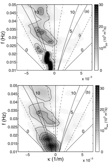
T. H. C. Herbers

Department of Oceanography, Naval Postgraduate School, Monterey, California, USA

Received 5 December 2003; revised 16 August 2004; accepted 18 November 2004; published 4 January 2005. [1] The infragravity wave (periods between roughly 20 and 200 s) energy balance in

shallow, nearshore waters is believed to be effected by generation by groups of sea and swell, dissipation, shoreline reflection, and refractive trapping. Observations obtained with alongshore oriented arrays of current meters or pressure gauges have been previously used to identify concentrations of energy at the frequency-alongshore wavenumbers of refractively trapped edge waves, but seaward and shoreward propagating waves were not differentiated. Surfzone dissipation theoretically limits edge wave growth, and a different analysis (using the approximation of shore-normal propagation) shows that the energy flux of shoreward propagating infragravity waves decreases owing to surfzone dissipation. Here an estimator is developed that yields the alongshore wavenumber-frequency spectra of seaward and shoreward propagating waves, using the WKB approximation and observations from an alongshore-oriented array of pressure and velocity sensors. Example spectra, estimated using data from the spatially sparse and relatively short SandyDuck arrays, suggests that strong dissipation of shoreward propagating infragravity waves occurs over a wide range of alongshore wavenumbers, effectively suppressing the excitation of edge wave modes.

Citation: Sheremet, A., R. T. Guza, and T. H. C. Herbers (2005), A new estimator for directional properties of nearshore waves, J. Geophys. Res.,110, C01001, doi:10.1029/2003JC002236.

1. Introduction

[2] Infragravity waves, with periods (between roughly 20 and 200 s) longer than sea and swell (between about 2 – 20 s), are ubiquitous on ocean shorelines. Generation by groups of sea and swell, dissipation, shoreline reflection, and refractive trapping have all been suggested to contribute significantly to the infragravity energy balance in shallow, nearshore waters [e.g., Munk, 1949; Longuet-Higgins and Stewart, 1962;Gallagher, 1971;Suhayda, 1974;Huntley et al., 1981; Herbers et al., 1995a, 1995b; Ruessink, 1998; Henderson and Bowen, 2002, 2003; Janssen and Battjes, 2003;Battjes et al., 2004]. A new method is presented here for analyzing the wave energy balance using array measure-ments of pressure and velocity.

[3] Some earlier studies of the infragravity energy bal-ance assumed approximately shore-normal propagating long waves. In this approximation, collocated observations of pressure (p) and cross-shore velocity (u) can be com-bined to estimate the time series of sea surface elevation associated with shoreward and seaward propagating waves (h±, respectively) h¼1 2 pu ffiffiffiffiffiffiffiffi h=g p ; ð1Þ

where h is the depth and g is gravitational acceleration [e.g., Guza et al., 1984; Elgar and Guza, 1985; List, 1992]. Frequency spectra of shoreward and seaward directed energy fluxes can be expressed as functions of thep,uauto- and cross-spectra. A case example from the SandyDuck experiment (Figure 1), conducted on a straight, gently sloped beach near Duck, North Carolina, shows the expected significant decrease in shoreward sea-swell energy flux within the surf zone (Figure 2a, x less than 230 m), and low energy levels of seaward 1_{Also at Department of Oceanography and Coastal Sciences, Louisiana}

State University, Baton Rouge, Louisiana, USA. Copyright 2005 by the American Geophysical Union. 0148-0227/05/2003JC002236$09.00

Public reporting burden for the collection of information is estimated to average 1 hour per response, including the time for reviewing instructions, searching existing data sources, gathering and maintaining the data needed, and completing and reviewing the collection of information. Send comments regarding this burden estimate or any other aspect of this collection of information, including suggestions for reducing this burden, to Washington Headquarters Services, Directorate for Information Operations and Reports, 1215 Jefferson Davis Highway, Suite 1204, Arlington VA 22202-4302. Respondents should be aware that notwithstanding any other provision of law, no person shall be subject to a penalty for failing to comply with a collection of information if it does not display a currently valid OMB control number.

1. REPORT DATE

2005 2. REPORT TYPE

3. DATES COVERED

00-00-2005 to 00-00-2005

4. TITLE AND SUBTITLE

A New Estimator for Directional Properties of Nearshore Waves

5a. CONTRACT NUMBER 5b. GRANT NUMBER

5c. PROGRAM ELEMENT NUMBER

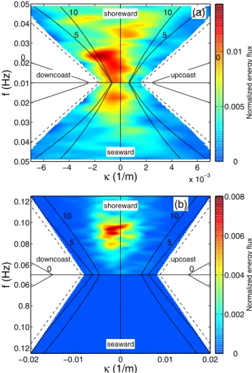
6. AUTHOR(S) 5d. PROJECT NUMBER

5e. TASK NUMBER 5f. WORK UNIT NUMBER 7. PERFORMING ORGANIZATION NAME(S) AND ADDRESS(ES)

Coastal Studies Institute,Louisiana State University,Baton Rouge,LA

8. PERFORMING ORGANIZATION REPORT NUMBER

9. SPONSORING/MONITORING AGENCY NAME(S) AND ADDRESS(ES) 10. SPONSOR/MONITOR’S ACRONYM(S) 11. SPONSOR/MONITOR’S REPORT NUMBER(S)

12. DISTRIBUTION/AVAILABILITY STATEMENT

Approved for public release; distribution unlimited

13. SUPPLEMENTARY NOTES 14. ABSTRACT

15. SUBJECT TERMS

16. SECURITY CLASSIFICATION OF: 17. LIMITATION OF ABSTRACT Same as Report (SAR) 18. NUMBER OF PAGES 11 19a. NAME OF RESPONSIBLE PERSON a. REPORT unclassified b. ABSTRACT unclassified c. THIS PAGE unclassified

Standard Form 298 (Rev. 8-98) Prescribed by ANSI Std Z39-18

propagating sea-swell waves. In contrast, the shoreward infragravity wave energy flux first increases (consistent with trapping and/or generation, Figure 2b) followed by a decrease in the inner surf zone (suggesting dissipation). A significant fraction of the shoreward infragravity energy reaches the shoreline and is strongly reflected, resulting in a mix of progressive and standing waves at all cross-shore locations (Figure 2c).

[4] Cross-shore patterns of energy flux variation qualita-tively similar to Figure 2 are observed often during the SandyDuck experiment [Sheremet et al., 2002]. Phase differences between pressure (or cross-shore velocity) ob-served at different cross-shore locations also suggest that sea-swell waves are predominantly shoreward progressive whereas infragravity waves are a mix of standing and shoreward progressive waves [Henderson and Bowen, 2002;Sheremet et al., 2002].

[5] Alongshore wavenumber-frequency (kf) spectra of p, u, or v (v is the alongshore velocity) often have been estimated using coherent analysis of observations obtained with an alongshore-oriented linear array [e.g., Munk et al., 1964]. The k f spectra of p estimated using the MEM (Maximum Entropy Method, Figure 3a), is elevated at f < 0.02 Hz for k within the theoretical range of low mode (<5) edge waves (Figure 3a). Edge waves, the normal modes of gravity waves undergoing complete, multiple reflections between the shoreline and the turning point (where jkj = kg = f/

ffiffiffiffiffi

gh

p

) have been hypothesized to be

preferentially excited relative tokfmodes that are off the edge wave dispersion curve [Gallagher, 1971]. Indeed, previous observations of alongshore velocity close to the shoreline sometimes show concentrations of energy at the

k f of low mode edge waves [Huntley et al., 1981; Oltman-Shay and Guza, 1987]. Dissipation at edge wave

k f theoretically reduces their resonant excitation [Henderson and Bowen, 2003], and the analysis using individual collocatedp,upairs (Figures 2b and 2c) suggests that a significant fraction of the shoreward propagating infragravity energy flux is dissipated.

[6] Two-dimensional arrays can provide estimates of the seaward and shoreward energy fluxes of directionally spread waves, but most existing methods assume a spatially homogeneous wave field [Elgar et al., 1994;Herbers et al., 1995b]. Inhomogeneity associated with phase coupling of seaward and shoreward propagating waves (standing wave patterns) can be neglected only if the array is located sufficiently far offshore of any reflector (e.g., the shoreline). This condition is often violated in surfzone experiments where measurements are collected within a few hundred meters of the shoreline. Phase-coupling between shoreward progressing and reflected waves is accounted for in the

Figure 1. (top) Plan view of SandyDuck instrument array

[Feddersen et al., 2000; Elgar et al., 2001]. Collocated pressure (p) and horizontal velocity (u, v) sensors are indicated (instruments were occasionally nonfunctional). The Field Research Facility coordinate frame is used, withx and y the cross-shore and alongshore directions. (bottom) Depth relative to MSL versus x is similar in August, September, and November (solid curves). The xorigin is a fixed onshore point, so the location of the mean shoreline varied with tide level and wave conditions.

Figure 2. Results for 10 September 1997, 0100 – 0400 EST

(Eastern Standard Time). The incident sea-swell peak period was about 12 s, with significant height of about 1 m. Assuming near-normal incidence (1), p and u sensors collocated at cross-shore locations along y = 828 m (Figure 1) are used to estimate frequency-band integrated seaward and shoreward energy fluxes for (a) sea swell (0.05 – 0.30 Hz), and (b) infragravity (0.01 – 0.05 Hz) waves. (c) Infragravity flux reflection coefficients (ratio of seaward to shoreward flux). (An erroneous date was given in the caption of Figure 3 [Sheremet et al., 2002]. The data presented in the group of panels on the right of that figure were collected on 12 October 1997, 1300 – 1600 EST.)

estimators of Isobe and Kondo [1984], but this method is designed for two-dimensional arrays of pressure gauges in uniform water depth.

[7] Here a method is developed that yields estimates of

k f spectra of shoreward and seaward energy fluxes in the k f region of (theoretically) refractively trapped infragravity waves. An extension of an existing method for a single p u gauge, the estimator uses the WKB approximation and observations from an alongshore (on a constant depth contour) array ofpugauges (Figure 1). The estimates are independent of phase-coupling between

shoreward and seaward propagating waves. A few exam-ple spectra, estimated using data from the spatially sparse and relatively short SandyDuck arrays, suggest that dis-sipation of shoreward propagating infragravity waves occurs over a wide range of alongshore wavenumbers, including those of (theoretically) refractively trapped edge waves.

2. Cross-Shore Energy Fluxes in Kf Space [8] The net cross-shore flux F of linear waves across a vertical section of unit width, oriented perpendicular to the wave propagation direction, is equal to the time-averaged (overbar), vertically integrated covariance ofpandu[e.g., Stoker, 1947],

F¼ Z 0

h

pudz; ð2Þ

where for the long waves considered here, p and u are independent of the vertical coordinatez.

[9] WithP, U, and V the double Fourier-Stieltjes trans-form from (x, y, t) space to (x, k, f) space, of pressure, cross-shore, and alongshore velocities, for example,

p xð ;y;tÞ ¼ Z1 1 Z1 1 e2piðkyþftÞdP xð ;k;fÞ; ð3Þ

the distributions of the variances and covariance ofp,u, and puinkfspace are

SPPdfdk¼2EhjdPj2i;

SUUdfdk¼2EhjdUj2i;

SPU dfdk¼2E½dPdU*;

ð4Þ

where E [ ] denotes the expected value, and the factor 2 arises from folding negative onto positive frequencies. The

kfspectral densities of pressure and cross-shore velocity (SPP and SUU) are real and positive, whereas the

cross-spectrumSPUis complex.

[10] Thekfspectra (4), that can be estimated with an alongshore array of p u gauges (section 3), can be combined into expressions for the distribution of wave energy and energy flux in the four quadrants defined by the shore-seaward and up-down coast directions. Assume a directionally spread wave field composed of onshore and offshore propagating WKB long waves [e.g.,Herbers et al., 1995a, 1995b;Sheremet et al., 2002],

dP xð ;k;fÞ ¼1 2 Aþðx;k;fÞe iqþðx;k;fÞ h þAðx;k;fÞeiqðx;k;fÞ i ; ð5Þ whereA±are the slowly varying, complex, local amplitude of shoreward (+) and seaward () propagating modes. Phase changes associated with propagation between the array location and the shoreline, and back to the array, are incorporated into the phase functionsq±.

Figure 3. Alongshore wavenumber-frequency (k f)

infragravity pressure spectra SPP, for 10 September 1997

(0100 – 0400 EST), using the alongshore array ofpsensors atx= 260 m (Figure 1) and (a) Maximum Entropy Method [Wu, 1997], and (b) new Hermite expansion method. Solid curves are edge wave dispersion relations for modes 0, 5, and 10, and dashed curves define turning points in the WKB approximation (jkj = kg= f/

ffiffiffiffiffi

gh

p

) that separate oscillatory and exponentially decaying cross-shore variations. The dash-dotted curves k = 2pf2/g separate trapped from leaky waves, assuming deep water offshore. Pressure time series (3 hours long) were sampled at 2 Hz, quadratically detrended, divided into 448-s-long demeaned ensembles with 50% overlap, and each ensemble was tapered with a Hanning window, yielding cross-spectra with about 48 degrees of freedom and frequency resolution of 0.002 Hz.

[11] Using (5) and the WKB relationship between pres-sure and horizontal velocitiesU= (ig/f)@P/@xyields

SPPdkdf ¼E 1 2 jAþj 2 þjAj2 h þ2Re AþA*eiðqþqÞ n oi ; ð6Þ SUUdkdf ¼E C 2 x 2h2 jAþj 2 þjAj2 h 2Re AþA*eiðqþqÞ n oi ; ð7Þ SPU dkdf ¼E jCxj 2h jAþj 2 þjAj2 h 2iIm AþA*eiðqþqÞ n oi ; ð8Þ where the superscript asterisk indicates complex conjugate,

Reand Im are the real and imaginary part of a complex variable, and the (x, k,f) dependence of A,Cx, and q are

dropped for brevity. Cx and Cy are the cross-shore and

alongshore components of the modal phase velocity C, given by the shallow water dispersion relation

C¼ðf=kÞk=k¼pffiffiffiffiffighk=k; ð9Þ where kx and k are the cross-shore and alongshore

components of the wavenumber vector k, and satisfy

jkj2= k2 = k2 + kx2.

[12] Up- and down-coast propagation inS_PPandS_UUare differentiated by the sign of k, but shoreward and seaward propagating energy are not distinguished (SPPandSUUare

symmetric in A+ and A). However, Re{SPU} is

propor-tional to differences in shoreward and seaward energy fluxes (jA+j2 jAj2) (8), and equals the net cross-shore

energy flux density in k f space. The co-spectrum of collocatedpusensors is equal to the cross-shore energy flux at frequency f, integrated over k. The integral of the puco-spectra over allfis equal to the net flux (2).

[13] Combining (6) – (8) yields, at each fandk, the vari-ance density of shoreward and seaward propagating modes,

E¼ E 1 2jAj 2 h i dfdk ¼ 1 4 SPP h Cx j j2Re SPUf g þ h2 C2 x SUU ð10Þ

and the corresponding cross-shore energy fluxes

F¼ h 4 Cx j j h SPP2Re SPUf g þ h Cx j jSUU : ð11Þ

The variance (10) and flux (11) estimates are independent of the phase coupling between shoreward and seaward propagating components. The sense of alongshore and cross-shore propagation is given by the signs of kandF±. For example,F+ withk> 0 corresponds to shoreward and up-coast propagation. Alongshore energy fluxes in k f space can be obtained by multiplying (10) by jCyj. These

results for long waves are readily extended using linear theory for finite depth.

[14] Gravity wave energy flux spectra can be estimated (using (11)) at locations where shear waves are energetic

because shear and gravity wave energies are concentrated in different regions of k f space. Shear waves propagate relatively slowly and satisfyjkj >kg, wherekg= f/

ffiffiffiffiffi

gh

p

is the theoretical maximum alongshore wavenumber for grav-ity waves [e.g., Oltman-Shay et al., 1989; Howd et al., 1991]. In contrast, shear waves degrade estimates of sea-ward and shoresea-ward gravity wave fluxes (1) based on time or frequency domain analysis of collocated p ugauges (cases with energetic shear waves were excluded from Sheremet et al.[2002]).

[15] Waves incident from deep water onto a shelf with plane parallel contours maintain constant k, where 0 <jkj < 2pf2/g. Waves withjkjslightly less than 2pf2/g propagate onto the shelf with highly oblique deep water angles, and waves withk0 are approximately normally incident. If excited in shallow water, waves with jkj < 2pf2/g can radiate (i.e., ‘‘leak’’) energy to deep water, reversing the ray path of waves incident from deep water, and are known as leaky waves [Munk et al., 1964]. Waves with jkj > f2/g cannot propagate in deep water, and if excited in shallow water, may undergo multiple, construc-tive reflections between the shoreline and an offshore turning point, wherek=kg=

ffiffiffiffiffi

gh

p

/f. These are refractively trapped edge waves. Edge waves are trapped (e.g., have a turning point) shoreward of the array ifk> kg. The curves

separating leaky from trapped waves (k = 2pf2/g), and separating edge waves trapped shoreward of the array from motions extending seaward of the array (k = kg), are

shown in Figure 3.

3. Application to Short Arrays

[16] At each frequency, spectral densities inkspace and cross-spectra (as observed with an alongshore array of sensors) form a Fourier pair, for example,

SPPð Þ ¼k Z1 1 XPPð ÞDe2pikDdD; XPPð Þ ¼D Z1 1 SPPð Þke2pikDdk; ð12Þ whereDis the alongshore lag andXis the cross-spectrum. However, because the arrays usually deployed (e.g., Figure 1) are relatively short compared with the alongshore wavelengths of interest, a direct Fourier transform of observed cross-spectra yields S(k) with unacceptably low resolution. For example, in 4-m water depth with f < 0.03 Hz the alongshore wavelength of the shortest free gravity wave (e.g., the maximum gravity wavenumber

k=kg=f/ ffiffiffiffiffi

gh

p

, indicated with a dashed line in Figure 3) is longer than the 200-m alongshore span of the array. (Shorter gravity waves with larger k, for example mode zero, are trapped shoreward of the array.) Thus the lowest Fourier

k band contains the entire range of theoretically possible free gravity wavek, including trapped and ‘‘leaky’’ waves incident from deep water [Munk et al., 1964].

[17] Increased k resolution requires additional assump-tions that essentially extend the array length by extrapolat-ing the observations. Widely used, ‘‘high-resolution’’ spectral estimators such as IMLE (Iterative Maximum Likelihood Estimator [Pawka, 1983]) and MEM (Maximum

Entropy Method, Figure 3a) are constrained to return positive-definiteS(k) and thus are not useful for estimating

Re{SPU}, that can have either sign.

[18] The alternative approach developed here is based on the assumption that the true cross-spectra decay at lags larger than those in the array, and that the true S(k) are smooth. The cross-spectra are expressed as a series of normalized Hermite functions, which form a complete and orthonormal basis [Weaver, 1989;Folland, 1992]. Hermite functionshnof ordernhave a strongly localized oscillatory

domain with nzero crossings separated by turning points from an outer region of rapid exponential decay (Figure 4). In addition to simple recursive properties, Hermite func-tions, like the Gaussian function (the lowest-order Hermite function), are self-reciprocal under the Fourier transform

Z1 1

hnð ÞDe2pikDdD¼ ð iÞnhnð Þk ; ð13Þ

simplifying considerably the procedure for finding solutions that satisfy simultaneously constraints in lag (fit the observed cross-spectra) and k(smoothS(k)) spaces.

[19] Since the estimate for F_± (equation 11) uses only the real part of SPU (SPP and SUU are real), only the

Hermitian part of the observed cross-spectra is needed. The Hermitian part ofX=Co+iQu, whereCoandQuare co- and quad-spectra, are approximated by sums of Her-mite functions, CoðDmÞ ¼ X n cnhnðDm=LÞ þðDmÞ;n¼0;2;. . .;2ðN1Þ QuðDmÞ ¼ X n cnhnðDm=LÞ þðDmÞ;n¼1;3;. . .;2N1; ð14Þ where is the misfit, and L is a scale factor used to nondimensionalize the lag variable of the Hermite func-tions, and the index midentifies the alongshore spatial lag (there areMlags). Even and odd Hermite orders are used to represent the (even) co- and (odd) quad-spectra, and the number Nof even and odd Hermite modes are equal.

[20] The finite number of cross-spectral observations can be fit closely with different sets of coefficientscn(14), and

some fits to the statistically noisy data result in wildly oscillating and nonphysicalS(k). FollowingConstable et al. [1987] andHerbers and Guza[1990], the total ‘‘badness’’ of the solution is minimized by solving

@ @cj aRþ T ¼0; ð15Þ

where the badness (aR+T) is the sum of a measure of the solution roughness aR, and the data misfitTwith the column vector of misfits at different lags and the superscript ( )Tdenotes the transpose. Straightforward algebra yields an analytic expression ((A11) in Appendix A) for the rough-nessR, characterized as the norm of the second derivative of S(k) ((A1) in Appendix A). TheCoorQuspectra observed at M lags are fit with a given tolerance using N Hermite coefficientscnthat simultaneously minimize the roughness

of the estimated S(k) (Appendix B). The contribution of Hermite modento the estimate roughnessRgrows roughly liken2(equation (A12) in Appendix A), so increasing the contribution of higher order Hermite modes improves the fit to the observed cross-spectra (e.g., decreases the misfit variance T), but increases R. Straightforward algebra yields a pair of equations for the coefficientsc, for example, forCo,

HT_HþaR

c¼HT_{Co; ð16Þ}

where c is the column vector (dimension N) of Hermite coefficients, andCois the column vector (dimensionM) of observed co-spectral values (14). The matrixH(dimension NM) has elements

H

½ lm¼hnðDm=LÞ; ð17Þ

where (from (14)) n = 2(l 1) for co-spectra and n = 2l 1 for quad-spectra. The roughness matrix R (dimension N N),

R¼cTRc; ð18Þ

(R is given in (A11)) has elements

R ½ li¼ qk qk4 dn;k4þ qk qk2 dn;k2þ q2 k q2 k2 þð2kþ1Þ2þq 2 kþ2 q2 k dn;kþ þqkþ2 qk dn;kþ2þ qkþ4 qk dn;kþ4; ð19Þ

where qn2 = n!, and for cospectra n = 2(l 1) and k =

2(i1), and for quad-spectran= 2l1 andk= 2i1 (14). [21] Equations (16), (17), and (19) form the basis of the method. Equation (16) can be solved using singular value decomposition methods [Strang, 1988] to obtain the coef-ficients cnof the decomposition (14) of the observedXPP,

XUU, and XPU. From the self-reciprocity (13), the

decom-position coefficients of the corresponding spectra (the Fourier transform of the cross-spectrum 12) are (i)ncn,

so estimates of the corresponding (k f) densities SPP,

SUU and SPU are readily available. For example,

SPUðkLÞ ¼X N1

k¼0

1

ð Þk½c2kh2kðkLÞ þc2kþ1h2kþ1ðkLÞ: ð20Þ

With SPP,SUUandSPUknown, equation (11) provides the

four-quadrant cross-shore fluxes.

[22] The scale factor L (17) maps the dimensional lag space observations into the space of the nondimensional Hermite variable. For each frequency the optimal values of L and the trade-off parameter a(15) are defined as those yielding, with a fixed number of Hermite modes, the Hermite-basedk-spectrum with minimum roughness that fits the observed cross-spectra with a given error (Appendix B). Results are not sensitive to the number of Hermite modes (here,N= 15), nor to details of the procedure for selectingL anda.

4. Results

[23] MEM estimates are positive, so MEM cannot be used to estimateSPU, or energy flux spectra that depend on

SPU (11). MEM and Hermite estimates of SPP are

qualita-tively similar at all frequencies (infragravity frequencies are shown in Figure 3). The cross-spectra associated with both MEM and Hermite estimates fit the observed cross-spectra closely (Figure 5, left), so their differences (Figure 5, right) reflect how each estimator resolves uncertainty (both statis-tical and arising from the limited array length) inherent in the basic cross-spectral observations. The estimates differ most at the lowest frequency (Figure 5b) because the long wavelength motions (Figure 5a) severely limit the array resolution. The MEM estimate is narrower than the Hermite-based estimate, reflecting the different properties of each method: high peak resolution in MEM and estimated smoothness in the present method. The estimate similarity increases at higher frequencies because the shorter wavelengths are better constrained by the obser-vations, decreasing the importance of differences in the estimator extrapolations.

[24] Example full (four-quadrant) cross-shore energy flux density spectra (Figures 6 – 8) are shown at the alongshore array locatedx= 260 m (in about 4-m depth) for three 3-hour runs with much different incident sea-swell significant heights (in 8-m water depth, about 1 km offshore,Hsig,8m=

Figure 5. Comparison of MEM (solid curves) and Hermite (dashed curves) estimators atx= 260 m at

frequencies (a, b) 0.01, (c, d) 0.025, (e, f ) 0.05, (g, h) 0.08 (spectral peak), and (i, j) 0.12 Hz. (left) Estimated pressure co-spectra XPPversus alongshore lagD (observations are shown as circles).

Quad-spectrum estimates show similar features. (right) EstimatedkfspectraSPPof pressure. The spectra are

normalized to unit area, integrated overk. Dashed vertical lines mark the turning-point limits of the WKB validity domain (jkj= f/pffiffiffiffiffigh). Note that thekscales vary by a factor of 10 between Figures 5b and 5j.

0.3, 0.9, and 1.7 m for 15 August, 10 September, and 17 October, respectively (Table 1). The observed cross-shore variation of sea-swell energy fluxes (similar to Figure 2a) suggests that the array at x = 260 m is located many surfzone widths offshore, near the outer edge of the surf-zone, and in the inner surfsurf-zone, respectively. On 15 August and 10 September, wave breaking seaward of the array is minimal, and the wave height observed at the array in 4-m depth Hsig,4m is slightly greater than Hsig,8m, whereas

breaking reduces Hsig,4m on 17 October to 1.1 m, only

slightly larger thanHsig= 1.0 m on 10 September (Table 1).

In all cases, shoreward propagating sea and swell is strongly dissipated in the surfzone shoreward of the array. The seaward swell flux is less than 3% of the seaward sea-swell flux at the array on 10 September and 17 October

(Figures 7b and 8b). Stronger reflection,10%, is observed on 15 August (Figure 6b) with small incident waves at high tide, when the water line intersects a steep portion of the beach face, consistent with previous observations at this site obtained with a two-dimensional array of pressure sensors in 13m water depth [Elgar et al., 1994].

[25] At infragravity frequencies, the flux reflection coef-ficientRig2 (ratio of seaward to shoreward fluxes) is

influ-enced by generation shoreward of the array, as well as dissipation occurring during both propagation and shoreline reflection [Herbers et al., 1995a, 1995b]. If, onshore of the array, generation exceeds dissipation, thenRig2 > 1, whereas

if dissipation exceeds generation,Rig2 < 1.

[26] Estimates of four-quadrant infragravity energy flux allow calculation of the k f distribution of the flux reflection coefficient. To avoid spurious reflection values at k f where fluxes are low and the estimates are inaccurate, and to increase the statistical stability of the estimates, fluxes are integrated over each of the k f regions of elevated shoreward flux. Seaward fluxes are integrated over the same regions of kfspace consistent with the observed specular reflection. For example, on

Figure 7. Cross-shore energy flux density inkfspace

atx= 260 m, for 10 September 1997, 0100 – 0400 EST for (a) infragravity and (b) sea-swell frequencies. Densities are normalized by the total shoreward flux (sea swell and infragravity fluxes are 3.4 105 and 1.4 104 cm3/s, respectively). Figure is same format as Figure 6.

Figure 6. Cross-shore energy flux density inkfspace

at x = 260 m, for 15 August 1997, 0100 – 0400 EST for (a) infragravity and (b) sea-swell frequencies. Edge wave dispersion curves for modes 0, 5, and 10 are solid curves, and dashed lines are the limit of validity for the WKB approximation (jkj= kg=f/

ffiffiffiffiffi

gh

p

). Densities are normalized by the total shoreward flux (sea swell and infragravity fluxes are 2.6 104 and 5.8 102 cm3/s, respectively) so the integrated shoreward flux is 1.0, and the integrated seaward flux isR2. The maximum color scale value is determined by the maximum normalized density. In Figures 6a and 6b, at fixedf, seaward and shoreward fluxes have maxima at similar

10 September, Rig

2

are between about 0.3 and 0.6 for frequency bands centered at f = 0.013, 0.019, 0.028, and 0.040 Hz (Figure 7). Flux spectra at other alongshore arrays also show negligible sea-swell reflection, and suggest specular, partial reflection of infragravity waves.

[27] The other case examples have H_sig,8mabout a factor of 2 larger (17 October) and smaller (15 August) than on 10 September. In all three cases, infragravity wave reflection is specular and incomplete. On 17 October, the large sea-swell waves are closer to normal incidence than on 10 September

(i.e., the energy maxima is closer tok= 0) and so are the infragravity waves (compare Figure 8 with Figure 7). The Rig2 0.5 are similar (Table 1). With the smallest waves

(10 September),Rig2 0.7 is higher, but dissipation is still

significant. Edge wave growth is apparently suppressed by significant dissipation within a wave cycle, supporting earlier work by Henderson and Bowen [2002, 2003]. Results from these case examples and the entire data set will be explored further elsewhere.

5. Discussion

[28] The WKB-based estimator (6 – 8) assumes that grav-ity waves, either leaky or refractively trapped, dominate the motions observed in the bandjkj<kg=f/

ffiffiffiffiffi

gh

p

. In the WKB approximation, observed alongshore velocities are theoret-ically redundant withpandu,

SVV ¼C 2 y h2SPP; SPV ¼ Cy h SPP; SUV ¼ Cy hSPU: ð21Þ

Estimates ofSVVbased directly onv, and onpmeasurements

using (21), are similar (Figures 9a, 9b, 9d, and 9e), as are the corresponding v energy spectra (Figures 9c and 9f, estimated by integrating SVV over k), supporting the

underlying assumptions. Differences are largest at infra-gravity frequencies (Figures 9a and 9b), where the directly measuredSVV(Figure 9a) is less concentrated alongk=kg

than the estimate based on the measured SPP and WKB

theory. The present WKB-based theory is problematic when

k kg and cross-shore flux estimates are not shown near

the dashed curve in Figures 6 – 8. However, directly measured infragravity pressure spectraSPP, estimated

with-out WKB theory, usually have maxima at k < kg and

relatively low energy whenkkg(Figure 3). Considering

all the arrays operational during the three case example runs, the variance with kkgaccounts for an average of

7% and a maximum of 9% of the total pressure variance (integrated overkand infragravity f).

[29] The WKB relationship between p and u (6 – 8), critical to the estimator, is based on the assumption of slowly varying depth, with the wave amplitude given by energy conservation and the wavenumber by constant-depth solutions. The linear shallow water equations relax the slowly varying assumption, and the bottom slope appears explicitly. Comparison of WKB wavenumbers and ampli-tudes with those obtained numerically from the shallow water equations for a normally incident shoreward progres-sive wave (Figure 10) indicates less than 10% error in WKB theory for all frequencies considered here (f > 0.01 Hz)

Figure 8. Cross-shore energy flux density inkfspace

at x = 260 m, for 17 October 1997, 0100 – 0400 EST for (a) infragravity and (b) sea-swell frequencies. Densities are normalized by the total shoreward flux (sea swell and infragravity fluxes are 4.2 105 and 1.8 104 cm3/s, respectively). Figure is same format as Figure 7.

Table 1. Wave Characteristics for the Case Examples, Measured at the FRF Array in 8-m Depth, and in About 4-m Depth atx= 260 ma Run,

Eastern Standard Time

Hsig,8m Sea Swell, m Hsig,4m Sea Swell, m Hsig,4m Infragravity, m urms,4m Sea Swell, m/s urms,4m Infragravity, m/s Rig 2 Infragravity 15 August 1997, 0100 – 0400 0.3 0.3 0.06 0.1 0.03 0.7 10 September 1997, 0100 – 0400 0.9 1.0 0.3 0.4 0.1 0.5 17 October 1997, 0100 – 0400 1.7 1.1 0.3 0.5 0.2 0.5 a

See Figure 1. Estimates of the significant wave heightHsig, root-mean square velocity fluctuationurms, and flux reflection coefficientR2are based on

for x > 210 m, and for f > 0.022 Hz at the shallowest alongshore array (x= 160 m).

6. Summary

[30] A new method for estimating wave energy fluxes from array observations is described. Under the WKB approximation, pressure and cross-shore velocity measured on an alongshore-oriented transect yield the distribution of onshore and offshore energy fluxes in alongshore wave-number-frequency space. Preliminary analysis of data from the spatially sparse and relatively short SandyDuck arrays shows that dissipation of shoreward propagating infragrav-ity waves occurs over a wide range of alongshore wave-numbers, including those of (theoretically) refractively trapped edge waves.

Appendix A: Roughness

[31] We derive an exact analytic expression for the roughness Rof thefkyspectrum S(f,k). The analytical

form greatly simplifies the solution of the equations for the coefficientscn.

[32] The roughness of S(f,k) is [Constable et al., 1987]

R fð Þ ¼ Z1 1 d2_{S fð ;kÞ} dk2 2 dk: ðA1Þ

Hermite functions of modenare [Weaver, 1989]

hnð Þ ¼t 1_{ffiffiffiffiffiffi} 4p p n ept2 d n dtn e 2pt2 ; ðA2Þ

with the first four modes

h0ð Þ ¼t ept 2 ; h1ð Þ ¼t ffiffiffiffiffiffi 4p p t ept2; h2ð Þ ¼t 4pt21 ept2 h3ð Þ ¼t ffiffiffiffiffiffi 4p p t h i3 pffiffiffiffiffiffi4pt ept2 ðA3Þ

and the recursive relation

hnþ1ð Þ ¼t 2 ffiffiffip

p

t hnð Þ t nhn1ð Þt ; ðA4Þ

wherehj= 0,j< 0.

[33] Hermite functions are also solutions of the Sturm-Liouville differential equation

h_n00ð Þ ¼t 2p2pt2ð2nþ1Þhnð Þt; ðA5Þ

where h00_n is the second derivative of Hermite mode n. Combining (A4) and (A5) yields

h_n00¼p hnþ2ð2nþ1Þhnþn nð 1Þhn2

: ðA6Þ

Figure 9. Alongshore velocitykfspectraSVVatx= 260 m for 10 September (estimated using Hermite

transforms) based on (a, d)vcross-spectra, and (b, e)pcross-spectra (WKB theory, SPPCy2/h2, (21)),

for (top) infragravity and (bottom) sea-swell frequencies. Solid curves are edge wave dispersion relations for modes 0, 5, and 10, and dashed curves define turning points in the WKB approximation (jkj = kg= f/

ffiffiffiffiffi

gh

p

). Results are shown for (jkj < f/pffiffiffiffiffigh). (c, f) Alongshore velocity frequency spectra Ev at x= 260 m estimated by integrating (over jkj < f/

ffiffiffiffiffi

gh

p

) SVV (Figures 9a and 9d) and SPPCy2/h2

Using Z1 1 h2ndt¼ n! ffiffiffi 2 p ðA7Þ

to normalize, the set of orthonormal Hermite functions is

hn¼ 4ffiffiffi₂ p ffiffiffiffi n! p hn; with Z1 1 hnð Þthmð Þtdt¼ dm;n; ðA8Þ

where dis the Kronecker symbol.

[34] Using (13), the Fourier transformg(t) of a functionG decomposed into Hermite functions G=Scnhnis

g tð Þ ¼X

1

n¼1

i

ð Þncnhnð Þt: ðA9Þ

The roughness (A1) is

R¼ Z1 1

g00ð Þt ½g00ð Þt *dt; ðA10Þ

where the superscript asterisk denotes complex conjugate. After some straightforward algebra using (A2) – (A6),

R¼p2X n cn qn qn4 cn4 þ qn qn2 cn2 þ q 2 n q2 n2 þð2nþ1Þ2þq 2 nþ2 q2 n cnþ þqnþ2 qn cnþ2þ qnþ4 qn cnþ4 ; ðA11Þ where qn 2

= n!, the range ofn is given by (14), and terms vanish if they containqnorcnwith negativen. For example,

qn=qn4¼ ffiffiffiffiffiffiffiffiffiffiffiffiffiffiffiffiffiffiffiffiffiffiffiffiffiffiffiffiffiffiffiffiffiffiffiffiffiffiffiffiffiffiffiffiffiffi n nð 1Þðn2Þðn3Þ p ; for n4 0; otherwise: 8 < : ðA12Þ

Appendix B: ParametersA and L

[35] The scale factor L (B1) maps the dimensional lag space observations into the nondimensional Hermite vari-able space (14). Optimal values ofLmatch the spatial scales of Hermite functions and the observed cross-spectra, and thus fit the observations efficiently (e.g., using low modes with low roughness). Values ofLthat are too large squeeze the entire lag domain of the observations into a small interval near the Hermite origin, and too small values spread the observed lag domain far out into the Hermite exponen-tial decay region (Figure 4). Here L is related to a fixed point characterizing the Hermite functions, the turning point tT’0.40 of the Gaussianh0(t), and the maximum lagDM,

L¼sDM

tT ; ðB1Þ

where s is the fraction of DM mapped into the Hermite

interval [0, tT]. A typical value of s = 0.4 yields DM/L =

2.5tT’1; that is, in (14) the observed cross-spectra are fit

with Hermite functions spanning the range t 1 (see Figure 4).

[36] For simplicity, for each frequency the optimal values of s (and hence L) and the tradeoff parameter a (15) are defined as those yielding the Hermite-based k-spectrum with minimum roughness and fitting the observed cross-spectra within a given error. More rigorous approaches, based on the statistical confidence level of the fit [Long and Hasselmann, 1979], are more complex and require esti-mates of the error-covariance matrix. Optimal (s,a) values were found for each cross-spectral combination ofpandu, at each array, and each frequency. Large a values have smoothS(k) but large misfit (15). For a givens, the optimal

a(denotedas) is the maximum value ofa(e.g., smoothest

S(k)) for which the misfit is within 1% of the cross-spectral norm. For a given frequency, the optimal (minimum rough-ness) solution is found by searching (s,as) pairs oversin

the interval of [0.1 – 10]. Optimal values of s are usually between 0.1 and 0.6, and are frequency dependent, with the largest values (and hence smallestDM/L) at low frequency

where the observed cross-spectra are most slowly varying (i.e., spatial scales are longest).

Figure 10. Contours of fractional errors in WKB estimates

of (a) amplitude and (b) wavenumber based on comparison with exact solutions to the linear shallow water equations for a shoreward propagating, normally incident wave using (c) depth h versus cross-shore coordinate x observed on 10 September.

[37] Acknowledgments. Funding was provided by the Office of Naval Research, the National Science Foundation, and the National Oceanographic Partnership Program (NOPP) program. Steve Elgar and Britt Raubenheimer contributed substantially to all aspects of the Sandy-Duck field program.

References

Battjes, J. A., H. J. Bakkenes, T. T. Janssen, and A. R. van Dongeren (2004), Shoaling of subharmonic gravity waves,J. Geophys. Res.,109, C02009, doi:10.1029/2003JC001863.

Constable, S., R. L. Parker, and C. Constable (1987), Occam’s inversion: A practical algorithm for generating smooth models from electromagnetic sounding data,Geophysics,52(3), 289 – 300.

Elgar, S., and R. T. Guza (1985), Observations of bispectra of shoaling surface gravity waves,J. Fluid Mech.,161, 425 – 448.

Elgar, S., T. H. C. Herbers, and R. T. Guza (1994), Reflection of ocean surface gravity waves from a natural beach,J. Phys. Oceanogr.,24(7), 1503 – 1511.

Elgar, S., R. T. Guza, W. C. O’Reilly, B. Raubenheimer, and T. H. C. Herbers (2001), Observations of wave energy and directions near a pier, J. Waterw. Port Coastal Ocean Eng.,127, 2 – 6.

Feddersen, F., R. T. Guza, S. Elgar, and T. H. C. Herbers (2000), Velocity moments in alongshore bottom stress parameterizations,J. Geophys. Res.,105, 8673 – 8686.

Folland, G. B. (1992),Fourier Analysis and Its Applications, Wadsworth, Stamford, Conn.

Gallagher, B. (1971), Generation of surf beat by non-linear wave interac-tions,J. Fluid Mech.,49, 1 – 20.

Guza, R. T., E. B. Thornton, and R. A. Holman (1984), Swash on steep and shallow beaches, paper presented at 19th Coastal Engineering Confer-ence, Am. Soc. of Civ. Eng., Houston, Texas.

Henderson, S. M., and A. J. Bowen (2002), Observations of surf beat forcing and dissipation,J. Geophys. Res.,107(C11), 3193, doi:10.1029/ 2000JC000498.

Henderson, S. M., and A. J. Bowen (2003), Simulations of dissipative, shore-oblique infragravity waves,J. Phys. Oceanogr.,33, 1722 – 1732. Herbers, T. H. C., and R. T. Guza (1990), Estimation of directional wave

spectra from multi-component observations, J. Phys. Oceanogr., 20, 1703 – 1724.

Herbers, T. H. C., S. Elgar, and R. T. Guza (1995a), Infragravity frequency (0.005 – 0.05 Hz) motions on the shelf: II. Free waves,J. Phys. Oceanogr., 25, 1063 – 1079.

Herbers, T. H. C., S. Elgar, and R. T. Guza (1995b), Generation and pro-pagation of infragravity waves,J. Geophys. Res.,100, 24,863 – 24,872. Howd, P. A., J. Oltman-Shay, and R. A. Holman (1991), Wave variance

partitioning in the trough of a barred beach,J. Geophys. Res., 96, 12,781 – 12,795.

Huntley, D. A., R. T. Guza, and E. B. Thornton (1981), Field observations of surf beat: 1. Progressive edge waves,J. Geophys. Res.,86, 6451 – 6466. Isobe, M., and K. Kondo (1984), Method for estimating directional wave

spectrum in incident and reflected wave field, paper presented at 19th Coastal Engineering Conference, Am. Soc. of Civ. Eng., Houston, Texas.

Janssen, T., and A. Battjes (2003), Long waves induced by short-wave groups over a sloping bottom, J. Geophys. Res., 108(C8), 3252, doi:10.1029/2002JC001515.

List, J. H. (1992), A model for the generation of two-dimensional surf beat, J. Geophys. Res.,97, 5623 – 5636.

Long, R. B., and K. Hasselmann (1979), A variational technique for extracting directional spectra from multi-component wave data,J. Phys. Oceanogr.,9, 373 – 381.

Longuet-Higgins, M. S., and R. W. Stewart (1962), Radiation stress and mass transport in surface gravity waves with application to ‘‘surf beats,’’ J. Fluid Mech.,13, 481 – 504.

Munk, W. H. (1949), Surf beat,Eos Trans. AGU,30, 849 – 854. Munk, W., F. Snodgrass, and F. Gilbert (1964), Long waves on the

continental shelf: An experiment to separate trapped and leaky modes, J. Fluid Mech.,20, 529 – 553.

Oltman-Shay, J., and R. T. Guza (1987), Infragravity edge wave observa-tions on two California beaches,J. Phys. Oceanogr.,17, 644 – 663. Oltman-Shay, J., P. Howd, and W. Birkemeier (1989), Shear instabilities of

the mean longshore current: 2. Field observations,J. Geophys. Res.,94, 18,031 – 18,042.

Pawka, S. (1983), Island shadows in wave directional spectra,J. Geophys. Res.,88, 2579 – 2591.

Reniers, A., A. van Dongeren, J. Battjes, and E. Thornton (2002), Linear modeling of infragravity waves during Delilah, J. Geophys. Res., 107(C10), 3137, doi:10.1029/2001JC001083.

Ruessink, B. G. (1998), Bound and free infragravity waves in the nearshore zone under breaking and non-breaking conditions,J. Geophys. Res.,103, 12,795 – 12,805.

Sheremet, A., R. T. Guza, S. Elgar, and T. H. C. Herbers (2002), Observations of nearshore infragravity waves: Seaward and shoreward propagating com-ponents,J. Geophys. Res.,107(C8), 3095, doi:10.1029/2001JC000970. Stoker, J. J. (1947),Water Waves, Wiley-Intersc., Hoboken, N. J. Strang, G. (1988),Linear Algebra and Its Applications, 3rd ed., Harcourt

Brace, San Diego, Calif.

Suhayda, J. N. (1974), Standing waves on beaches,J. Geophys. Res.,79, 3065 – 3071.

Van Dongeren, A., A. Reniers, J. Battjes, and I. Svendsen (2003), Numerical modeling of infragravity wave response during DELILAH, J. Geophys. Res., 108(C9), 3288, doi:10.1029/2002JC001332. Weaver, H. J. (1989),Theory of Discrete and Continuous Fourier Analysis,

John Wiley, Hoboken, N. J.

Wu, N. (1997),The Maximum Entropy Method, Springer-Verlag, New York.

R. T. Guza, Integrative Oceanography Division, Scripps Institution of Oceanography, University of California, San Diego, La Jolla, CA 92093-0209, USA. ([email protected])

T. H. C. Herbers, Department of Oceanography, Naval Postgraduate School, Monterey, CA 93943-5122, USA. ([email protected])

A. Sheremet, Coastal Studies Institute, Louisiana State University, Baton Rouge, LA 70803, USA. ([email protected])