Nonlinear Support Vector Machines through
Iterative Majorization and I-Splines
P.J.F. Groenen
∗G. Nalbantov
†J.C. Bioch
∗July 19, 2006
Econometric Institute Report EI 2006-25 Abstract
To minimize the primal support vector machine (SVM) problem, we propose to use iterative majorization. To do so, we propose to use it-erative majorization. To allow for nonlinearity of the predictors, we use (non)monotone spline transformations. An advantage over the usual ker-nel approach in the dual problem is that the variables can be easily inter-preted. We illustrate this with an example from the literature.
Keywords: Support vector machines, Iterative majorization, I-Splines.
1
Introduction
In recent years, support vector machines (SVMs) have become a popular tech-nique to predict two groups out of a set of predictor variables (Vapnik, 2000). This data analysis problem is not new and such data can also be analyzed through alternative techniques such as linear and quadratic discriminant anal-ysis, neural networks, and logistic regression. However, SVMs seem to compare favorably in their prediction quality with respect to competing models. Also, their optimization problem is well defined and can be solved through a quadratic program. Furthermore, the classification rule derived from an SVM is relatively simple and it can be readily applied to new, unseen samples. At the downside, the interpretation in terms of the predictor variables in nonlinear SVM is not always possible. In addition, the usual formulation of an SVM is not easy to grasp.
In this paper, we offer a different way of looking at SVMs that makes the interpretation much easier. First of all, we stick to the primal problem and ∗Econometric Institute, Erasmus University Rotterdam, P.O. Box 1738, 3000 DR Rotter-dam, The [email protected],[email protected]
†ERIM, Erasmus University Rotterdam, P.O. Box 1738, 3000 DR Rotterdam, The [email protected]
formulate the SVM in terms of a loss function that is regularized by a penalty term. From this formulation, it can be seen that SVMs use robustified errors. Then, we propose a new majorization algorithm that minimizes the loss. Finally, we show how nonlinearity can be imposed by using I-Spline transformations.
2
The SVM Loss Function
In many ways, an SVM resembles regression quite closely. Let us first introduce some notation. LetXbe then×m matrix of predictor variables ofnobjects andmvariables. The n×1 vectorycontains the grouping of the objects into two classes, that is, yi = 1 if objecti belongs to class 1 andyi =−1 if object
ibelongs to class−1. Obviously, the labels−1 and 1 to distinguish the classes are unimportant. Letwbe them×1 vector with weights used to make a linear combination of the predictor variables. Then, the predicted valueqi for object
iis
qi=c+x0iw, (1)
wherex0
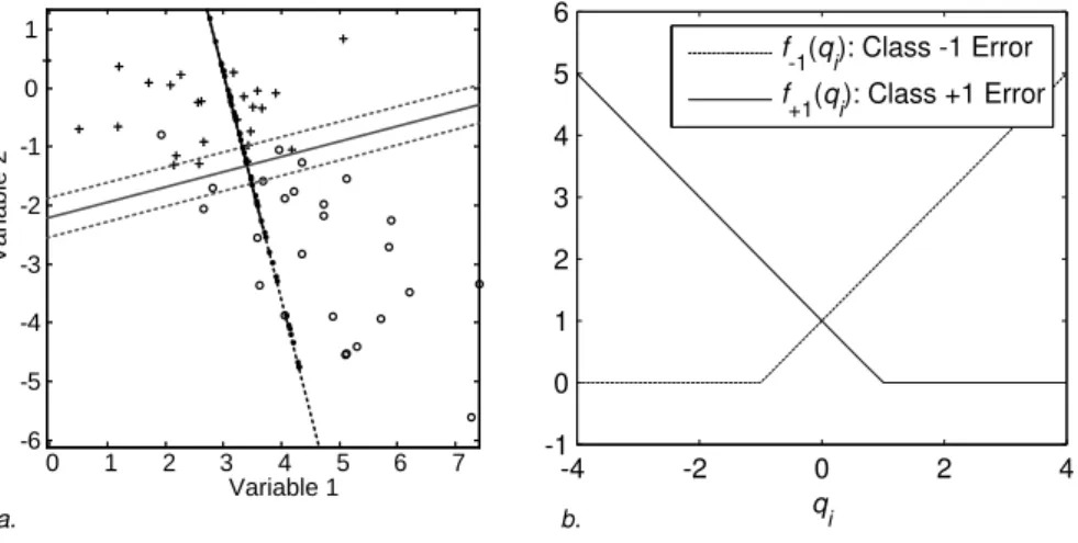
iis rowiofXandcis an intercept. Consider the example in Figure 1a
where for two predictor variables, each rowi is represented by a point labelled ‘+’ for the class 1 and ‘o’ for class−1. Every combination ofw1andw2defines a direction in this scatter plot. Then, each pointican be projected onto this line. The idea of the SVM is to choose this line in such a way that the projections of the class 1 points are well separated from those of class −1 points. The line of separation is orthogonal to the line with projections and the intercept
c determines where exactly it occurs. Note that if w has length 1, that is, kwk= (w0w)1/2= 1, then Figure 1a explains fully the linear combination (1). If w has not length 1, then the scale values along the projection line should be multiplied by kwk. The dotted lines in Figure 1a show all those points that project to the lines atqi =−1 and qi = 1. These dotted lines are called
the margin lines in SVMs. Note that if there are more than two variables the margin lines become hyperplanes. Summarizing, the SVM has three sets of parameters that determines its solution: (1) the regression weights, normalized to have length 1, that is,w/kwk, (2) the length ofw, that is,kwk, and (3) the interceptc.
SVMs count an error as follows. Every object i from class 1 that projects such thatqi≥1 yields a zero error. However, ifqi<1, then the error is linear
with 1−qi. Similarly, objects in class−1 withqi≤ −1 do not contribute to the
error, but those with qi >−1 contribute linearly withqi+ 1. In other words,
objects that project on the wrong side of their margin contribute to the error, whereas objects that project on the correct side of their margin yield zero error. Figure 1b shows the error functions for the two classes.
As the length ofw controls how close the margin lines are to each other, it can be beneficial for the number of errors to choose the largestkwkpossible, so that fewer points contribute to the error. To control the kwk, a penalty term
0 1 2 3 4 5 6 7 -6 -5 -4 -3 -2 -1 0 1 Variable 1 Va ria ble 2 -4 -2 0 2 4 -1 0 1 2 3 4 5 6 q i f -1(qi): Class -1 Error f +1(qi): Class +1 Error b. a.
Figure 1: Panel a Projections of the observations in groups 1 (+) and−1 (o) onto the line given byw1 and w2. Panel b shows the error functionf1(qi) for
class 1 objects (solid line) andf−1(qi) for class−1 objects (dashed line).
that is dependent onkwkis added to the loss function. The penalty term also avoids overfitting of the data.
LetG1and G−1denote the sets of class 1 and −1 objects. Then, the SVM loss function can be written as
LSVM(c,w) = Pi∈G1max(0,1−qi) + P i∈G−1max(0, qi+ 1) + λw 0w = Pi∈G1f1(qi) + P i∈G−1f−1(qi) + λw 0w
= Class 1 errors + Class−1 errors + Penalty for,
nonzerow
(2)
see, for similar expressions, Hastie, Tibshirani, and Friedman (2000) and Vapnik (2000).
Assume that a solution has been found. All the objects i that project on the correct side of their margin, contribute with zero error to the loss. As a consequence, these objects could be removed from the analysis without changing the solution. Therefore, all the objectsithat project at the wrong side of their margin and thus induce error or if an object falls exactly on the margin, then these objects determine the solution. Such objects are called support vectors as they form the fundament of the SVM solution. Note that these objects (the support vectors) are not known in advance so that the analysis needs to be carried out with allnobjects present in the analysis.
What can be seen from (2) is that any error is punished linearly, not quadrat-ically. Thus, SVMs are more robust against outliers than a least-squares loss function. The idea of introducing robustness by absolute errors is not new. For
more information on robust multivariate analysis, we refer to Huber (1981), Vapnik (2000), and Rousseeuw and Leroy (2003).
The SVM literature usually presents the SVM loss function as follows (Burges, 1998): LSVMClas(c,w, ξ) = C X i∈G1 ξi+C X i∈G2 ξi+1 2w 0w, (3) subject to 1 + (c+w0x i)≤ξi fori∈G−1 (4) 1−(c+w0xi)≤ξi fori∈G1 (5) ξi ≥0, (6)
whereCis a nonnegative parameter set by the user to weight the importance of the errors represented by the so-called slack variablesξi. Suppose that objecti
inG1 projects at the right side of its margin, that is,qi =c+w0xi ≥1. As a
consequence, 1−(c+w0x
i)≤0 so that the correspondingξi can be chosen as
0. Ifiprojects on the wrong side of its margin, thenqi=c+w0xi<1 so that
1−(c+w0x
i)>0. Choosingξi= 1−(c+w0xi) gives the smallestξi satisfying
the restrictions in (4), (5), and (6). As a consequence,ξi= max(0,1−qi) and
is a measure of error. A similar derivation can be made for class −1 objects. ChoosingC= (2λ)−1gives LSVMClas(c,w, ξ) = (2λ)−1 X i∈G1 ξi+ X i∈G−1 ξi+ 2λ1 2w 0w = (2λ)−1 X i∈G1 max(0,1−qi) + X i∈G−1 max(0, qi+ 1) +λw0w = (2λ)−1L SVM(c,w).
showing that the two formulations (2) and (3) are exactly the same up to a scaling factor (2λ)−1 and yield the same solution. However, the advantage of (2) is that it can be interpreted as a (robust) error function with a penalty. The quadratic penalty term is used for regularization much in the same way as in ridge regression, that is, to force thewj to be close to zero. The penalty is
particularly useful to avoid overfitting. Furthermore, it can be easily seen that
LSVM(c,w) is a convex function in candw because all three terms are convex incandw. As the function is also bounded below by zero and it is convex, the minimum of LSVM(c,w) is a global one. In fact, (3) allows the problem to be treated as a quadratic program. However, in the next section, we optimize (2) directly by the method of iterative majorization.
3
A Majorizing Algorithm for SVM
In the SVM literature, the dual of (3) is reexpressed as a quadratic program and is solved by special quadratic program solvers. A disadvantage of these solvers is that they may become computationally slow for large number of objects n
(although fast specialized solvers exist). However, here we derive an iterative majorization (IM) algorithm. An advantage of IM algorithms is that each it-eration reduces (2). As this function is convex and IM is a guaranteed descent algorithm, the IM algorithm will stop when the estimates are sufficiently close to the global minimum.
Letf(q) be the function to be minimized. Iterative majorization operates on an auxiliary function, called the majorizing functiong(q,q), that is dependent onqand the previous (known) estimateq. The majorizing functiong(q,q) has to fulfill several requirements: (1) it should touchf at the supporting pointy, that is,f(q) =g(q,q), (2) it should never be belowf, that is, f(q)≤g(q,q), and (3)g(q,q) should be simple, preferably linear or quadratic inq. Letq∗ be
such thatg(q∗,q)≤g(q,q), for example, by finding the minimum of g(q,q).
Because the majorizing function is never below the original function, we obtain the so called sandwich inequality
f(q∗)≤g(q∗,q)≤g(q,q) =f(q)
showing that the update q∗ obtained by minimizing the majorizing function
never increasesf and usually decreases it. More information on iterative ma-jorization can be found in De Leeuw (1994), Heiser (1995), Lange, Hunter, and Yang (2000), Kiers (2002), and Hunter and Lange (2004) and an introduction in Borg and Groenen (2005).
To find an algorithm, we need to find a majorizing function for (2). First, we derive a quadratic majorizing function for each individual error term. Then, we combine the results for all terms and come up with the total majorizing function that is quadratic inc andw so that an update can be readily derived. At the end of this section, we provide the majorization results.
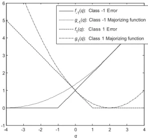
Consider the term f−1(q) = max(0, q+ 1). For notational convenience, we drop the subscripti for the moment. The solid line in Figure 2 showsf−1(q). Because of its shape of a hinge, this function is sometimes referred to as the hinge function. Let q be the known error q of the previous iteration. Then, a majorizing function for f−1(q) is given by g−1(q, q) at the supporting point q = 2. For notational convenience, we refer in the sequel to the majorizing function as g−1(q) without the implicit argument q. We want g−1(q) to be quadratic so that it is of the form g−1(q) = a−1q2 −2b−1q+c−1. To find a−1, b−1, and c−1, we impose two supporting points, one at q and the other at−2−q. These two supporting points are located symmetrically around−1. Note that the hinge function is linear at both supporting points, albeit with different gradients. Becauseg−1(q) is quadratic, the additional requirement that f−1(q)≤g−1(q) is satisfied ifa−1>0 and the derivatives at the two supporting points off−1(q) andg−1(q) are the same. More formally, the requirements are
-4 -3 -2 -1 0 q 1 2 3 4 -1 0 1 2 3 4 5 6 f-1(q): Class -1 Error
g-1(q): Class -1 Majorizing function f1(q): Class 1 Error
g1(q): Class 1 Majorizing function
Figure 2: The error functions of Groups−1 and 1 and their majorizing functions. The supporting point isq= 2. Note that the majorizing function for Group−1 also touches atq=−4 and that of Group 1 also at 0.
that f−1(q) = g−1(q), f0 −1(q) = g−0 1(q), f−1(−2−q) = g−1(−2−q), f0 −1(−2−q) = g−0 1(−2−q), f−1(q) ≤ g−1(q). It can be verified that the choice of
a−1 = 14|q+ 1|−1, (7)
b−1 = −a−1−14, (8)
c−1 = a−1+21+14|q+ 1|, (9)
satisfies all these requirements. Figure 2 shows the majorizing functiong−1(q) with supporting pointsq= 2 orq=−4 as the dotted line.
For Group 1, a similar majorizing function can be found forf1(q) = max(0,1− q). However, in this case, we require equal function values and first derivative atqand at 2−q, that is, symmetric around 1. The requirements are
f1(q) = g1(q), f0 1(q) = g10(q), f1(2−q) = g1(2−q), f0 1(2−q) = g10(2−q), f1(q) ≤ g1(q).
Choosing
a1 = 14|1−q|−1 b1 = a1+14
c1 = a1+12+14|1−q|
satisfies these requirements. The functions f1(q) and g1(q) with supporting pointsq= 2 orq= 0 are plotted in Figure 2.
Note thata−1is not defined ifq=−1. In that case, we choosea−1as a small positive constantδthat is smaller than the convergence criterion²(introduced below). Strictly speaking, the majorization requirements are violated. How-ever, by choosingδsmall enough, the monotone convergence of the sequence of
LSVM(w) will be no problem. The same holds fora1 ifq= 1. Let ai = ½ max(δ, a−1i) ifi∈G−1, max(δ, a1i) ifi∈G1, (10) bi = ½ b−1i ifi∈G−1, b1i ifi∈G1, (11) ci = ½ c−1i ifi∈G−1, c1i ifi∈G1. (12)
Then, summing all the individual terms leads to the majorization inequality
LSVM(c,w) ≤ n X i=1 aiqi2−2 n X i=1 biqi+ n X i=1 ci+λ m X j=1 w2 j. (13)
Becauseqi =c+x0iwi, it is useful to add an extra column of ones as the first
column ofXso thatX becomesn×(m+ 1). Letv0= [cw0] so thatq=Xv.
Now, (2) can be majorized as
LSVM(v) ≤ n X i=1 ai(x0iv)2−2 n X i=1 bix0iv+ n X i=1 ci+λ mX+1 j=2 v2j = v0X0AXv−2v0X0b+c m+λv0Kv = v0(X0AX+λK)v−2v0X0b+c m, (14)
where A is a diagonal matrix with elements ai on the diagonal, bis a vector
with elements bi, and cm =
Pn
i=1ci, and K is the identity matrix except for
element k11 = 0. Differentiation the last line of (14) with respect to v yields the system of equalities linear inv
(X0AX+λK)v=X0b.
The update v+ solves this set of linear equalities, for example, by Gaussian elimination, or, somewhat less efficiently, by
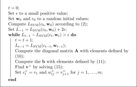
t= 0;
Set²to a small positive value;
Setw0 andc0 to a random initial values; ComputeLSVM(c0,w0) according to (2); SetL−1=LSVM(c0,w0) + 2²;
whileLt−1−LSVM(ct,wt)> ²do
t=t+ 1;
Lt−1=LSVM(ct−1,wt−1);
Compute the diagonal matrixAwith elements defined by (10);
Compute thebwith elements defined by (11); Findv+ by solving (15);
Setc+t =v1 andwtj+ =v+j+1 forj= 1, . . . , m; end
Figure 3: The SVM majorization algorithm.
Because of the substitutionv0 = [c w0], the update of the intercept isc+ =v 1
and w+j = v+j+1 for j = 1, . . . , m. The update v+ forms the heart of the
majorization algorithm for SVMs.
The majorizing algorithm for minimizing the standard SVM in (2) is sum-marized in Figure 3. This algorithm has several advantages. First, it iteratively approaches the global minimum closer in each iteration. In contrast, quadratic programming of the dual problem need to solve the dual problem completely to have the global minimum of the original primal problem. Secondly, the progress can be monitored, for example, in terms of the changes in the number of misclas-sified objects. Thirdly, to reduce the computational time, smart initial estimates ofcandw can be given if they are available, for example, from a previous cross validation run.
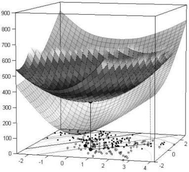
An illustration of the iterative majorization algorithm is given in Figure 4. Here,cis fixed at its optimal value and the minimization is only overw, that is, overw1andw2. Each point in the horizontal plane represents a combination of w1andw2. The majorization function is indeed located above the original func-tion and touches it at the dotted line. Thew1 andw2 where this majorization function finds its minimum,LSVM(c,w) is lower than at the previous estimate, so LSVM(c,w) has decreased. Note that the separation line and the margins corresponding to the current estimates of w1 and w2 are given together with the class 1 points represented as open circles and the class−1 points as closed circles.
Figure 4: Example of the iterative majorization algorithm for SVMs in action wherec is fixed andw1andw2are being optimized. The majorization function touchesLSVM(c,w) at the previous estimates ofw(the dotted line) and a solid line is lowered at the minimum of the majorizing function showing a decrease inLSVM(c,w) as well.
4
Nonlinear SVM
The SVM described so far tries to find a linear combinationq=Xbsuch that negative values are classified into class−1 and positive values into class 1. As a consequence, there is a separation hyperplane of all the points that project such that q= 0. Therefore, the standard SVM has a linear separation hyperplane. To allow for a nonlinear separation plane, the the classical approach is to turn to the dual problem and introduce kernels. By doing so, the relation with the primal problemLSVM(c,w) is lost and the interpretation in terms of the original variables is not always possible anymore.
To cover nonlinearity, we use the optimal scaling ideas from Gifi (1990). In particular, each predictor variable is being transformed. A powerful class of transformations is formed by spline transformation. The advantage of splines
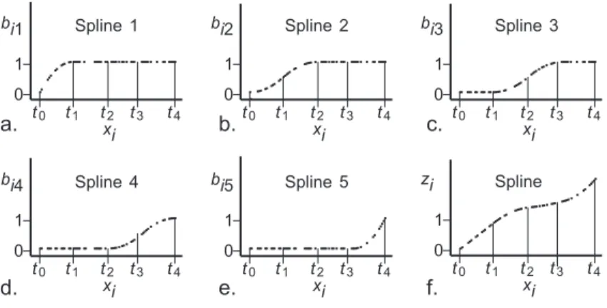
bi 1 0 1 t0 t1 t2 t3 t4 ... ... ... Spline 1 xi xi bi 2 0 1 t0 t1 t2 t3 t4 ..... .. ... Spline 2 xi bi 3 0 1 t0 t1 t2 t3 t4 ... ... ... Spline 3 xi zi 0 1 t0 t1 t2 t3 t4 Spline xi bi4 0 1 t0 t1 t2 t3 t4 ... ... ... Spline 4 xi Spline 5 bi5 0 1 t0 t1 t2 t3 t4 ... ... .... ... ... ... ... a. b. c. d. e. f.
Figure 5: Panels a to e give an example of the columns of the spline basisB. It consists of five columns given the degreed= 2 and the number of interior knots
k= 3. Panel f shows a linear sum of these bases that is the resulting I-Spline transformationzfor a single predictor variablex.
is that they yield transformations that are piecewise polynomial. In addition, the transformation is smooth. Because the resulting transformation consists of polynomials whose coefficients are known, the spline basis values can also be computed for unobserved points. Therefore, the transformed value of test points in can be easily computed.
There are various sorts of spline transformations, but here we choose the I-Spline transformations (see Ramsay, 1988). An example of such a transforma-tion is given in Figure 5f. In this case, the piecewise polynomial consists of four intervals. The boundary points between subsequent intervals are called interior knots tk. The interior knots are chosen such that the number of observations
is about equal in each interval. The degree of the polynomialdin the I-Spline transformation of Figure 5f is 2 so that each piece is quadratic in the original predictor variablexj. Once the number of interior knotskand the degreedare
fixed, each I-Spline transformation can be expressed aszj =Bjwj whereBj is
the so called spline basis ofn×(d+k). For the example transformation in Figure 5f, the columns ofBj are visualized in Figures 5a to 5e. One of the properties
of the I-Spline transformation is that if the weightswjare all positive, then the
transformation is monotone increasing as in our example as in Figure 5f. This property is of use to interpret the solution.
To estimate the transformations in the SVM problem, we simply replaceX
by the matrixB= [B1 B2 . . . Bm], that is, by concatenating the spline bases
Bj, one for each original predictor variablexj. In our example, we havem= 2
variables (x1andx2),d= 2, andk= 3, so thatB1andB2are both matrices of sizen×(d+k) =n×5 andBis of sizen×m(d+k) =n×10. Then, the vector of weightsw0= [w0
1w02 . . . w0m] is of sizem(d+k)×1 and the transformationzj
-2 -1 0 1 2 3 4 -2 -1.5 -1 -0.5 0 0.5 1 1.5 2 2.5 3 x1 x2 -2 -1 0 1 2 3 4 -2 -1.5 -1 -0.5 0 0.5 1 1.5 2 2.5 3 x1 x2
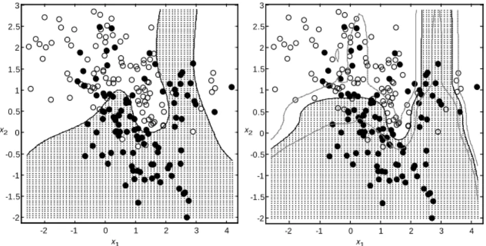
Figure 6: The left panel shows samples from a mixture distribution of two groups (Hastie et al., 2000) and a sample of points of these groups. The line is the optimal Bayes decision boundary. The right panel shows the SVM solution using spline transformations of degree 2 and 5 interior knots,λ=.00316, with an training error rate of .21.
in the decision boundary, we extend the space of predictor variables fromXto the space of the spline bases of all predictor variables and then search through the SVM for a linear separation in this high dimensional space.
Consider the example of a mixture of 20 distributions for two groups given by Hastie et al. (2000) on two variables. The left panel of Figure 6 shows a sample 200 points with 100 in each class. It also shows the optimal Bayes decision boundary. The right panel of Figure 6 shows the results of the SVM with I-Spline transformations of the two predictor variables using k = 5 and d = 2. After cross validation, the best preformingλ=.00316 yielding a training error rate of .21.
Once the SVM is estimated andwis known, the transformationszj=Bjwj
are determined. Thus, each interval of the transformation is in our example with
d= 2 a quadratic function in xj for which the polynomial coefficients can be
derived. As test points, we use a grid in the space of the two predictor variables. Because the polynomial coefficients are known for each interval, we can derive the transformed (interpolated) valuezij of test pointifor eachj and the value
qi =c+
P
jzij where c is the intercept. Ifqi for the test point is positive, we
classify the test pointiin class 1, ifqi<0 in class−1, and ifqi= 0 it is on the
decision boundary. This classification is done for all the test points in the grid, resulting in the reconstructed boundary in the right panel of Figure 6.
I-Splines have the property that for nonnegativewthe transformationzj is
monotone increasing withxj. Let wj+ = max(0,wj) and w−j = min(0,wj) so
-5 0 5 0 5 10 15 20 x1 Positive transformation -5 0 5 -15 -10 -5 0 5 Negative transformation x1 -2 0 2 4 -5 0 5 10 x2 Positive transformation -2 0 2 4 -5 0 5 10 Negative transformation x2 z1+ z1 -z2+ z2
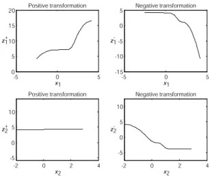
-Figure 7: Spline transformations of the two predictor variables used in the SVM solution in the right panel of Figure 6.
increasing partz+
j =Bjwj+ and a monotone decreasing partz−j =Bjw+j. For
the mixture example, these transformations are shown in Figure 7 for each of the two predictor variables. From this figure, we see that forx1the nonlinearity is caused by the steep transformations of values forx1>1 both for the positive as for the negative part. Forx2, the nonlinearity seems to be caused by only by the negative transformation forx2<1.
5
Conclusions
We have discussed how SVM can be viewed as a the minimization of a robust error function with a regularization penalty. Nonlinearity was introduced by mapping the space of each predictor variable into a higher dimensional space using I-Spline basis. The regularization is needed to avoid overfitting in the case when the number of predictor variables increases or the their respective spline bases become of high rank. The use of I-Spline transformations are useful to allow interpreting the nonlinearity in the prediction. We also provided a new majorization algorithm for the minimization of the primal SVM problem.
There are several open issues and possible extensions. A disadvantage of the I-Spline transformation over the usual kernel approach is that the degree of the spline d and the number of interior knots k need to be set whereas most standard kernels just have a single parameter. We need more numerical experience to study what good ranges for these parameters are.
The present approach can be extended to other error functions as well. Also, there seems to be close relations with the optimal scaling approach taken in multidimensional scaling and by the work of Gifi (1990). We intend to study
these issues in subsequent publications.
References
Borg, I., & Groenen, P. J. F. (2005). Modern multidimensional scaling: Theory
and applications (2nd edition). New York: Springer.
Burges, C. J. C. (1998). A tutorial on support vector machines for pattern recognition. Knowledge Discovery and Data Mining, 2, 121–167.
De Leeuw, J. (1994). Block relaxation algorithms in statistics. In H.-H. Bock, W. Lenski, & M. M. Richter (Eds.),Information systems and data analysis
(pp. 308–324). Berlin: Springer.
Gifi, A. (1990). Nonlinear multivariate analysis. Chichester: Wiley.
Hastie, T., Tibshirani, R., & Friedman, J. (2000). The elements of statistical
learning. New York: Springer.
Heiser, W. J. (1995). Convergent computation by iterative majorization: Theory and applications in multidimensional data analysis. In W. J. Krzanowski (Ed.),Recent advances in descriptive multivariate analysis (pp. 157–189). Oxford: Oxford University Press.
Huber, P. J. (1981). Robust statistics. New York: Wiley.
Hunter, D. R., & Lange, K. (2004). A tutorial on MM algorithms.The American Statistician,39, 30–37.
Kiers, H. A. L. (2002). Setting up alternating least squares and iterative ma-jorization algorithms for solving various matrix optimization problems.
Computational Statistics and Data Analysis,41, 157–170.
Lange, K., Hunter, D. R., & Yang, I. (2000). Optimization transfer using surrogate objective functions. Journal of Computational and Graphical Statistics,9, 1–20.
Ramsay, J. O. (1988). Monotone regression splines in action.Statistical Science,
3(4), 425–461.
Rousseeuw, P. J., & Leroy, A. M. (2003).Robust regression and outlier detection.
New York: Wiley.
Vapnik, V. N. (2000). The nature of statistical learning theory. New York: Springer.