ADAPTIVE BASIS SAMPLING FOR SMOOTHING SPLINES
A Dissertation by NAN ZHANG
Submitted to the Office of Graduate and Professional Studies of Texas A&M University
in partial fulfillment of the requirements for the degree of DOCTOR OF PHILOSOPHY
Chair of Committee, Jianhua Huang Committee Members, Raymond J. Carroll
Mohsen Pourahmadi Joel Zinn
Head of Department, Valen E. Johnson
August 2015
Major Subject: Statistics
ABSTRACT
Smoothing splines provide flexible nonparametric regression estimators. Penal-ized likelihood method is adopted when responses are from exponential families and multivariate models are constructed with certain analysis of variance decomposition. However, the high computational cost of smoothing splines for large data sets has hindered their wide application. We develop a new method, named adaptive ba-sis sampling, for efficient computation of smoothing splines in super-large samples. Generally, a smoothing spline for a regression problem with sample size n can be expressed as a linear combination of n basis functions and its computational com-plexity isO(n3). We achieve a more scalable computation in the multivariate case by evaluating the smoothing spline using a smaller set of basis functions, obtained by an adaptive sampling scheme that uses values of the response variable. Our asymp-totic analysis shows that smoothing splines computed via adaptive basis sampling converge to the true function at the same rate as full basis smoothing splines. We show that the proposed method outperforms a sampling method that does not use the values of response variable by simulation studies, and apply it to several real data examples.
ACKNOWLEDGEMENTS
I would like to express my deepest gratitude to my advisor Jianhua Huang, for his guidance and support throughout my doctoral studies. Professor Huang has been a source of constant personal encouragement and intellectual stimulation not only during the research work but over the five years I have been at Texas A&M. It is my honor to be able to work with him.
My thanks also extend to the other members of my committee, Raymond Carroll, Mohsen Pourahmadi and Joel Zinn, for their interest and insightful comments. I would like to thank Ping Ma for initiating the research projects in this work and our collaboration is a fruitful experience.
I want to thank everyone in the Department of Statistics, including faculty, staff, visitors and my fellow graduate students. I feel fortunate to spend my five years in such a friendly and stimulating environment. In particular, I benefited greatly from many conversations with Anirban and interactions with members in our research group. I am also thankful to my friends outside the department, especially Hancheng, Fan, Bo and Gang. Life out of work is much more colorful with them.
Finally, I dedicate this work to my family: my parents, Dacheng Zhang and Yuexia Sun, and my fianc´ee, Ruoxin Wang, for their sacrifices and devotion. Their unconditional love and endless support have always been my strength.
TABLE OF CONTENTS Page ABSTRACT . . . ii DEDICATION . . . iii ACKNOWLEDGEMENTS . . . iv TABLE OF CONTENTS . . . v
LIST OF FIGURES . . . vii
LIST OF TABLES . . . ix
1. INTRODUCTION . . . 1
1.1 Background . . . 2
1.2 Main contribution . . . 4
2. REGRESSION WITH GAUSSIAN RESPONSES . . . 6
2.1 Introduction . . . 6
2.2 Smoothing splines and computational issues . . . 7
2.3 Sampling of basis functions . . . 10
2.3.1 Uniform sampling of basis functions . . . 10
2.3.2 Adaptive sampling of basis functions . . . 11
2.3.3 Efficient computation . . . 14
2.3.4 Bayesian confidence intervals . . . 16
2.4 Convergence rates for function estimation . . . 17
2.4.1 Regularity conditions . . . 17
2.4.2 Convergence rates . . . 19
2.5 Simulation results . . . 21
2.6 Real data example . . . 26
3. REGRESSION WITH RESPONSES FROM EXPONENTIAL FAMILIES 29 3.1 Introduction . . . 29
3.1.1 Estimating gene expression in RNA-Seq . . . 30 3.1.2 Genome-wide methylation analysis using bisulfite sequencing . 31
3.1.3 Exponential family smoothing spline ANOVA models . . . 32
3.2 Efficient computation of smoothing spline ANOVA models via adap-tive basis selection . . . 34
3.2.1 Penalized likelihood for fitting smoothing spline ANOVA models 35 3.2.2 Adaptive basis selection . . . 39
3.3 Asymptotic analysis . . . 42
3.3.1 Regularity conditions . . . 42
3.3.2 Rate of convergence . . . 44
3.3.3 The dimension of the effective model space . . . 45
3.4 Simulation study . . . 46
3.5 Real examples . . . 49
3.5.1 Modeling the time course gene expression profiles using RNA-Seq 49 3.5.2 Differentially methylated DNA regions in Arabidopsis . . . 54
3.6 Discussion . . . 56
4. PROPERTIES OF ADAPTIVE BASIS SAMPLING AND TECHNICAL PROOFS . . . 57
4.1 Basic theoretical properties of adaptive basis sampling . . . 57
4.2 Technical proofs . . . 60
4.2.1 Ancillary lemmas . . . 61
4.2.2 Proof of main results . . . 61
5. CONCLUSIONS . . . 72
LIST OF FIGURES
FIGURE Page
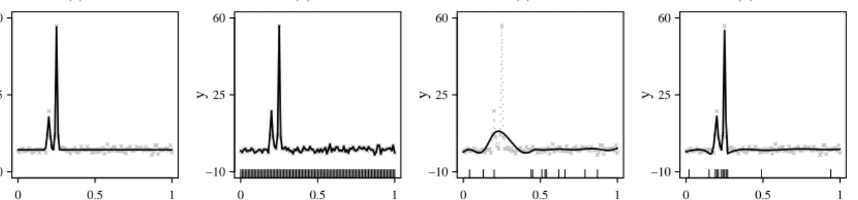
2.1 Toy regression function with two close peaks: (a) true signal (solid line) and 100 observations (gray crosses); (b) smoothing spline fit (solid line) with full basis; (c) smoothing spline fit (solid line) with 12 uniformly sampled basis functions (UBS); (d) smoothing spline fit (solid line) with 12 adaptively sampled basis functions (ABS). In (b)-(d), short vertical lines at the bottom mark the data points cor-responding to the selected basis functions; observations are indicated by gray crosses; true signal is shown as dotted gray lines. . . 11 2.2 Bivariate nonparanormal copula density function. (a): contour plot
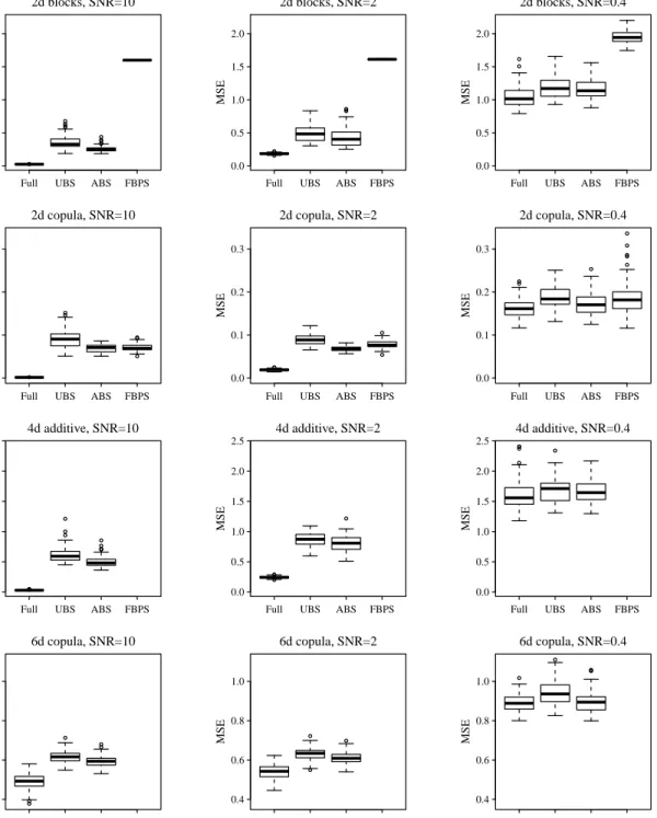
of true function; (b)–(c): contour plots of absolute values of fitting residuals by smoothing splines based on uniform basis sampling (UBS) and adaptive basis sampling (ABS). The sampled basis functions are marked by +’s. . . 13 2.3 Boxplots of the mean squared errors for four multivariate test
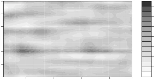
func-tions under three signal-to-noise ratios (SNR) (10,2,0.4), based on 100 simulation runs. Full, UBS and ABS stand for smoothing spline estimators with full basis, uniform basis sampling and adaptive basis sampling. FBPS is fast bivariate P-splines. . . 23 2.4 The estimated image of core-mantle boundary (CMB) region structure
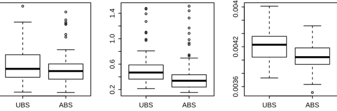
using smoothing spline with adaptive basis sampling. . . 28 3.1 Boxplots of MSE for multivariate simulation studies. Left: bivariate
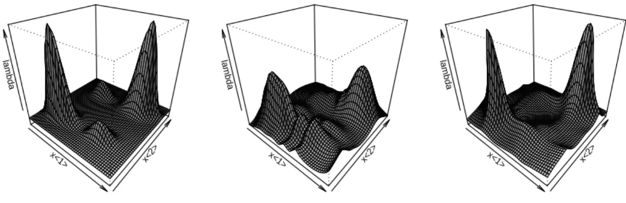
blocks function with negative binomial distribution; middle: bivariate copula density function with Poisson distribution; right: four dimen-sional copula density function with binomial distribution. UBS and ABS stand for smoothing spline ANOVA models estimator under uni-form and adaptive basis sampling strategies. . . 47 3.2 Bivariate blocks function with negative binomial distribution.
Per-spective plots of true probability, fitted values by smoothing splines via uniform basis sampling and adaptive basis sampling. . . 48
3.3 Bivariate copula density function with Poisson distribution. Perspec-tive plots of true mean parameter, fitted values by smoothing splines via uniform basis sampling and adaptive basis sampling. . . 48 3.4 Estimated counts after removing GC bias for two time courses of gene
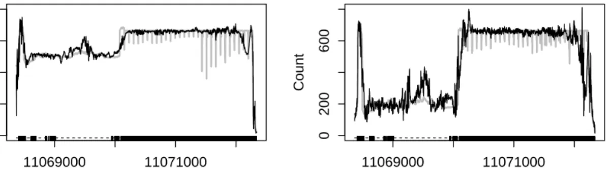
Hsc70-4. Observed counts are in gray line and black line is the esti-mation, the blocks in the bottom are exons. . . 52 3.5 Predicted counts after removing GC bias for two time courses of gene
Ef2b. Observed counts are in gray line and black line is the estimation, the blocks in the bottom are exons. . . 52 3.6 Mapped methylated read counts and fitted methylation level for a
whole genome bisulfite sequencing data of Arabidopsis thaliana. The grey lines at left panels are the mapped methylation read counts for four strains of two generations. The black lines are the fitted methyla-tion levels. The thick bars in x-axises are locamethyla-tion of genes AT2G17540 (left) and AT2G17550 (right) . . . 55
LIST OF TABLES
TABLE Page
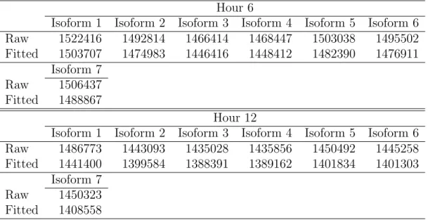
2.1 Means and standard errors (in parentheses) of computational time (in seconds) for four multivariate cases, based on 100 simulation runs. (SNR, signal-to-noise ratio; UBS, uniform basis sampling; ABS, adap-tive basis sampling; FBPS, fast bivariate P-splines.) . . . 25 3.1 Raw read counts and fitted counts for all 7 isoforms of gene Hsc70-4
at Hour 6 and 12. . . 53 3.2 Raw read counts and fitted counts for all 3 isoforms of gene Ef2b at
1. INTRODUCTION
Smoothing splines provide flexible nonparametric regression estimators. Due to several distinguished features, smoothing splines stand out as a popular choice among nonparametric modeling methods (Ruppert et al., 2003). First, it is conceptually simple. Smoothing spline is essentially a set of segmented low degree polynomials connected smoothly at some specified points. Second, its model-fitting is data-driven and does not require manual parameter-tuning. Smoothing spline treats each data point as a node and uses a penalized likelihood to fit the model with regularization parameters tuned by generalized cross-validation (Gu, 2013). Nevertheless, the high computational cost of smoothing splines for large data sets has hindered their wide application. For example, modern biology technologies can sequence tens of millions DNA/cDNA fragments in parallel. After the resulting sequences are mapped to genome, one gets a sequence of short read counts along genome. Smoothing splines have been used extensively for modeling and processing single sequencing sample. However, nonparametric joint modeling of multiple sequencing samples are still lack-ing due to expensive computational cost.
In this dissertation, we develop a new method, named adaptive basis sampling, for efficient computation of smoothing splines in large samples. Such basis sampling scheme makes use of information from response variable and is computationally ef-fective. We consider nonparametric regression with Gaussian and non-Gaussian re-sponses, and present a systematic treatment to analyze the asymptotic properties of the smoothing spline estimator with adaptively selected basis functions.
1.1 Background
To estimate a function of interestηon a generic domain X using stochastic data, one may use the minimizer of the penalized likelihood
L(η|data) +λ J(η), (1.1)
where L(η|data) is usually taken as negative log likelihood of the data and J(η) is a quadratic functional quantifying the roughness of η. The penalty parameter λ controls the trade-off between the goodness-of-fit and smoothness of η. See Wahba (1990), Gu (2013) and Wang (2011) for overviews of this method.
The standard formulation of smoothing splines performs the minimization of (1.1) in a reproducing kernel Hilbert space H ={η : J(η) <∞}, where J(·) is seen as a squared semi-norm. Let NJ ={η :J(η) = 0} be the null space of J(η) and assume
that NJ is a finite dimensional linear subspace of H. Denote by HJ the orthogonal
complement of NJ in H such that H = NJ ⊕ HJ. The reproducing kernel Hilbert
space provides a very general framework for nonparametric regression where the penalty term J(η) can be chosen to serve different purposes. For univariate function estimation on a compact interval X, one can use
J(η) =
Z
X
(η(m))2dx.
In particular, m = 2 corresponds to the commonly-used second derivative penalty and the minimizer of (1.1) is a natural cubic spline. For estimating a multivariate function on a compact domain X ⊂ Rd(d > 1), one can use the thin-plate spline
penalty Jmd(η) = Z · · · Z X X ν1+···+νd=m m! ν1!· · ·νd! ∂mη ∂xν1 1 · · ·∂x νd d 2 dx1· · ·dxd (1.2)
where m is the order of derivatives and d is the number of predictor variables (Duchon, 1977). As a special case, when m= 2 and d= 2 we have
J22(η) = Z Z X ∂2η ∂x2 1 2 + ∂2η ∂x1∂x2 2 + ∂2η ∂x2 2 2 dx1dx2.
See Gu (2013) for details about defining the penalty term and corresponding repro-ducing kernel Hilbert space for modeling a multivariate regression function using smoothing spline analysis of variance models.
Univariate smoothing splines can be computed in O(n) by applying the Reinsch (1967) algorithm. In general, as we shall see in the next chapter, the computational cost of finding the minimizer of (1.1) is in the order of O(n3) and thus is very large for big data sets. To lower the computational cost, over the past decades, there have been efforts to find sparse sets of basis functions to approximate the minimizer of (1.1). Luo and Wahba (1997) and Zhang et al. (2004) applied variable selection techniques, but it is not clear whether the resulting estimators share the good asymptotic properties of standard smoothing splines. Gu and Kim (2002) and Kim and Gu (2004) developed a simple random sampling approach for basis function selection and established a coherent theory for the convergence of their approximated smoothing splines. To overcome the computational burden of smoothing splines, pseudosplines (Hastie, 1996) and penalized splines (Ruppert et al., 2003) have also been proposed. Both use a small number of fixed basis functions to approximate the smoothing splines; they are similar in spirit to Gu and Kim (2002) and Kim and Gu
(2004) but differ in the construction of the basis functions. 1.2 Main contribution
Our adaptive basis sampling method for approximating smoothing splines is an extension of the simple random sampling approach of Gu and Kim (2002) and Kim and Gu (2004). Its novelty is that we select the basis functions according to the slicing along the range of the response variable. These adaptively selected basis functions form a reduced model space, called the effective model space. We compute the approximated smoothing spline estimator in the reduced space to achieve efficient computation. This adaptive sampling strategy differs from all existing methods based on sampling basis functions on the direction of the predictors. It can recover fine details of the response surface better than the simple random sampling scheme.
With the proposed basis sampling method, we achieve a more scalable computa-tion through a sparse approximacomputa-tion of smoothing spline ANOVA models in a lower dimensional effective model space. The asymptotic analysis shows that smoothing spline estimator computed via adaptive basis sampling converges at the same rate as that of full basis smoothing spline estimator. As evident in our simulation and real data analysis studies, smoothing spline ANOVA models approximation via adaptive basis selection provide very accurate estimates.
Chapter 2 is devoted to nonparametric regression with Gaussian responses. Ef-fective methods for smoothing parameter selection and generic algorithms for com-putation are the main topics. It is also focusing on the estimation of multivariate functions with large samples. Compared with other competing methods such as penalized spline, our approach is statistically more efficient according to both sim-ulation study and a read data example on geographical imaging analysis. Chap-ter 3 extends the adaptive basis sampling to a generalized regression problem, where
the response variables come from exponential family distributions. Motivated by two next-generation sequencing data sets, we are particularly interested in modeling counts data and thus responses are assumed to be Poisson, binomial or negative binomial distributed. Chapter 4 studies some theoretical properties of estimators constructed by the adaptive basis sampling method. Proofs of some lemmas and theorems in Chapter 2 and 3 are collected. Since Gaussian distribution is also an exponential family distribution, proofs for Chapter 2 are special cases of those of Chapter 3. We only present the general case.
2. REGRESSION WITH GAUSSIAN RESPONSES
2.1 Introduction Consider the nonparametric regression model
yi =η(xi) +i, i= 1, . . . , n (2.1)
where yi is the ith observation of the response variable, xi is the ith observation
of the predictor variable on the domain X ⊂ Rd (d ≥ 1), η is the nonparametric
function to be estimated, and the i’s are independent and identically distributed
random errors with mean zero and unknown constant variance σ2. A widely used method for estimating the unknown function η in (2.1) is via minimization of the penalized least squares criterion
PLS(η) = 1 n n X i=1 {yi−η(xi)}2+λ J(η), (2.2)
whereJ(η) is a quadratic functional quantifying the roughness ofη. The first term in expression (2.2) discourages lack of fit, and the second term penalizes the roughness ofη. The penalty parameterλcontrols the trade-off between the goodness-of-fit and smoothness ofη. Multivariate penalty parameters can be introduced when estimating a multivariate function, but we focus our presentation on the single penalty case. See Wahba (1990), Gu (2013) and Wang (2011) for overviews of this method, including how to introduce multivariate penalty parameters.
The standard formulation of smoothing splines performs the minimization of (2.2) in a reproducing kernel Hilbert space H ={η :J(η) <∞}, where J(·) is a squared semi-norm. Let NJ = {η : J(η) = 0} be the null space of J(η) and assume that
NJ is a finite dimensional linear subspace of H with basis {ξi :i= 1, . . . , m}, where
m = dim(NJ). Denote byHJ the orthogonal complement of NJ inH such thatH=
NJ ⊕ HJ. Let P be the orthogonal projection operator from H ontoHJ. Then J(·)
is a well-defined squared norm of HJ and for any η ∈ H, J(η) = J(P η) = kP ηk2HJ. With this norm, HJ is also a reproducing kernel Hilbert space, and we denote its
reproducing kernel by RJ(·,·).
In this chapter, we propose an adaptive basis sampling method for approximat-ing smoothapproximat-ing splines. We select the basis functions accordapproximat-ing to the response vari-able. These basis functions form an effective model space. Efficient computation is achieved when we compute the approximated smoothing spline estimator in the effective model space. In addition, we develop an asymptotic theory on the rate of convergence of our approximated smoothing spline estimator. This theory is non-standard because of the response-dependent sampling scheme, and yields conditions on the dimension of the effective model space to warrant the same convergence rate as the regular smoothing spline estimators. Such conditions provide useful practical guidelines for the sample size of the adaptive sampling.
2.2 Smoothing splines and computational issues
We first state the so-called representer theorem (e.g., Wahba, 1990), which de-clares that although the original penalized least squares problem for smoothing splines is formulated in the infinite-dimensional function spaceH={η:J(η)<∞}, the solution lies in a finite-dimensional space. Recall that H has the tensor-sum decomposition H = NJ ⊕ HJ, {ξi}mi=1 spans the null space NJ of the quadratic
functional J, and RJ(·,·) is the reproducing kernel of HJ.
Rn such that the minimizer of (2.2) over H can be represented as η(x) = m X k=1 dkξk(x) + n X i=1 ciRJ(xi, x), x∈ X. (2.3)
Theorem 2.2.1 implies that we need only search for the minimizer of (2.2) over the collection of functions of form (2.3), so the problem reduces to finding the coefficient vectorsdandcthat satisfy a system of linear equations. Letx= (x1, . . . , xn)>be the
vector of observed values of the predictor variable, andy= (y1, . . . , yn)>be the vector
of corresponding observations of the response variable. Let η ={η(x1), . . . , η(xn)}>
denote the n evaluations of η(·) at x, S denote the n×m matrix with the (i, j)th entry ξj(xi), andR denote then×n matrix with the (i, j)th entry RJ(xi, xj). Then
the decomposition (2.3) applied to x yields the system of equations
η=Sd+Rc, (2.4)
and thus the first term on the right-hand side of (2.2) becomes
n−1(y−Sd−Rc)>(y−Sd−Rc). (2.5)
On the other hand, for any function η with the expansion (2.3), the penalty function J(η) in (2.2) can also be written in a matrix form using the reproducing property of RJ(·,·), i.e.,
hRJ(xi,·), RJ(xj,·)iHJ =RJ(xi, xj).
Pn i=1ciRJ(xi,·). Hence J(η) =kP ηk2 HJ = DXn i=1 ciRJ(xi, x), n X i=1 ciRJ(xi, x) E HJ = n X i=1 n X j=1 ciRJ(xi, xj)cj =c>R c. (2.6)
Combining (2.5) and (2.6), we see that the penalized least squares criterion (2.2) is reduced to
PLS(η) = 1
n(y−Sd−Rc) >
(y−Sd−Rc) +λ c>R c. (2.7)
Since PLS(η) is a quadratic form in both d and c, its minimizer has a closed-form expression. Differentiating (2.7) with respect to d and cand setting the derivatives to zero, we obtain the linear system of equations
S>S S>R R>S R>R+nλR d c = S>y R>y . (2.8)
To solve this system, of size m+n, the computational cost is generally of the order O(n3), which can be prohibitive when the sample sizenis large. From Theorem 2.2.1, the number of basis functions used to represent the solution is m+n, which grows with n. While the m basis functions for NJ are needed, it may be not necessary to
use all nbasis functions forHJ. If a smaller number of basis functions can provide a
good approximation of the smoothing spline solution, then a computationally efficient algorithm can be developed to handle cases with large sample size. We discuss two sampling approaches for selecting basis functions in the next section.
2.3 Sampling of basis functions
2.3.1 Uniform sampling of basis functions
We first review an approach of selecting basis functions by randomly sampling the observations of the predictor variable and discuss its limitations, and then present our new sampling approach that involves the response variable.
From the representer theorem, each of the n basis functions for representing the function inHJ is uniquely associated with an observed value of the predictor variable.
Thus a natural idea for selecting the basis functions is through randomly sampling the observed values of the predictor variable. Specifically, we draw a random sample of sizen∗ from the observed predictor values{xi}ni=1, denoted as x∗ = (x∗1, . . . , x∗n∗)>,
and use the corresponding basis functions, {RJ(x∗i, x)}n ∗
i=1, to represent functions in HJ. We then solve the penalized least squares problem in the effective model space
HE = NJ ⊕span{RJ(x∗i, x), i = 1, . . . , n
∗}. When n∗ is much smaller than n, the computational cost can be significantly reduced.
Gu and Kim (2002) and Kim and Gu (2004) proved that this uniform sampling scheme has some nice theoretical properties. Under some reasonable conditions, the smoothing spline estimator computed under this scheme can achieve the same asymptotic convergence rate as the full basis smoothing spline estimator that uses all the basis functions indicated in the representer theorem.
When the number of sampled basis functions increases, the estimator from the uniform sampling strategy will approach the smoothing spline estimator and reveal the underlying true function. However, if constrained by computational resources, one may not sample enough basis functions to achieve a satisfactory result. Figure 2.1 illustrates this with a toy example. The underlying true function is the density function of a two-component mixture of normal distributions. Panel (c) shows the
(a) Truth x y −10 25 60 0 0.5 1 (b) Full x y −10 25 60 0 0.5 1 (c) UBS x y −10 25 60 0 0.5 1 (d) ABS x y −10 25 60 0 0.5 1
Figure 2.1: Toy regression function with two close peaks: (a) true signal (solid line) and 100 observations (gray crosses); (b) smoothing spline fit (solid line) with full basis; (c) smoothing spline fit (solid line) with 12 uniformly sampled basis func-tions (UBS); (d) smoothing spline fit (solid line) with 12 adaptively sampled basis functions (ABS). In (b)-(d), short vertical lines at the bottom mark the data points corresponding to the selected basis functions; observations are indicated by gray crosses; true signal is shown as dotted gray lines.
smoothing spline fit using 12 uniformly sampled basis functions, which does not reveal the two peaks of the mixture components because uniform sampling does not select the basis function corresponding to the point with the largest y-value. Unless the number of basis functions is greatly increased, there is little chance that the estimator can capture this peak.
2.3.2 Adaptive sampling of basis functions
We propose a new sampling scheme to select basis functions which makes use of the observed values of the response variable. This scheme may sample more basis functions in regions where the response function has big changes and sample fewer basis functions where the response surface is relatively flat. We call this new scheme adaptive basis sampling.
samples the basis functions from the collection{RJ(xi,·) :i= 1, . . . , n}as indicated
in the representer theorem. The difference is the way the sampling is performed. In adaptive basis sampling, we first group the xi’s according to the corresponding value
of the response variable, and then draw random samples within each group. The detailed procedure is given below.
1. Divide the range of the responses{yi}ni=1 intoK disjoint intervals, S1, . . ., SK.
Let |Sk| denote the number of observations inSk.
2. For eachSk, consider the collection of all pairs (xi, yi) whereyi ∈Sk, and draw
a random sample of size nk from this collection. Denote the sampled predictor
values by x∗(k) = (x1∗(k), . . . , x∗(nkk)).
3. Combine x∗(1), . . . , x∗(K) together to form a set of sampled predictor values {x∗
1, . . . , x ∗
n∗}. This set has size n∗ =PKk=1nk.
4. Form the effective model space
HE =NJ ⊕span{RJ(x∗j,·), j = 1, . . . , n
∗}.
(2.9)
Minimize the penalized least squares criterion (2.2) over this effective model space.
The first step of the adaptive basis sampling procedure groups together observa-tions with similar response values. It is the same operation as binning when con-structing histograms and slicing in sliced inverse regression (Li, 1991; Cook, 1998). Each set{(xi, yi) :yi ∈Sk}is referred to as a slice of the data. We expect this
(a) Truth −2 −1 0 1 2 −2 −1 0 1 2 x1 x2 0 2 4 + + + + + + + + + + + + + + + + + + + + + + + + + + + + + + + + + + + + + + + + + + + + + + + + + + + + (b) UBS −2 −1 0 1 2 −2 −1 0 1 2 x1 x2 0 1 2 + + + + + + + + + ++ + + + + + + + ++ + + + + + + + + + + + + + ++ + + + + + + + ++ + + + + ++ + + (c) ABS −2 −1 0 1 2 −2 −1 0 1 2 x1 x2 0 1 2
Figure 2.2: Bivariate nonparanormal copula density function. (a): contour plot of true function; (b)–(c): contour plots of absolute values of fitting residuals by smoothing splines based on uniform basis sampling (UBS) and adaptive basis sam-pling (ABS). The sampled basis functions are marked by +’s.
Figure 2.1(d) displays the smoothing spline fit from the adaptive sampling scheme with 12 basis functions. The fit reveals the two peaks of the mixture components well, since basis functions corresponding to the peak points are sampled.
To further illustrate how adaptive basis sampling works and compare it with uniform basis sampling, we considered a two-dimensional example for which the response surface is a bivariate nonparanormal copula density function; see §2.5 for its analytical form. Figure 2.2(a) depicts the contour plot of the true function, showing four peaks: two are significantly higher than the others. Contour plots of absolute values of residuals after smoothing spline fitting, presented in Fig. 2.2(b)-(c), indicate that the estimated two big peaks from adaptive basis sampling are closer to the truth than from uniform basis sampling. That adaptive basis sampling smoothing spline yields a better estimate can be explained by the distribution of
sampled basis functions, also shown in (b) and (c): the basis functions sampled by uniform basis sampling spread over the whole domain while those sampled by adaptive basis sampling are mainly distributed around the four peaks, especially the two significant ones.
In §2.4, we show that the adaptive sampling scheme can achieve the asymptotic rate of convergence of the original smoothing spline estimator, although a much smaller set of basis functions is employed. The theoretical results of Gu and Kim (2002) and Kim and Gu (2004) for uniform sampling cannot be applied to adaptive sampling, because values of the response variable are used in selecting the basis functions.
2.3.3 Efficient computation
We now present the details of the computational algorithm when adaptive basis sampling is used to compute the smoothing spline estimator. Recall that the selected data points are denoted by x∗ = (x∗1, . . . , x∗n∗)>. Under adaptive basis sampling, the
minimizer of (2.2) is approximated by ηA(x) = m X k=1 dkξk(x) + n∗ X j=1 cjRJ(x∗j, x).
We letS denote then×mmatrix with (i, j)th entryξj(xi). LetR∗ be an×n∗ matrix
with the (i, j)th entryRJ(xi, x∗j) andR∗∗ be a n∗×n∗ matrix with the (i, j)th entry
RJ(x∗i, x
∗
j). If we rearrange the original data by putting the selected data points x
∗ at the front, R∗ is just the left part of R while R∗∗ is the top-left corner of R. The evaluations of ηA at locations x, ηA={ηA(x1), . . . , ηA(xn)}>, satisfy
where dA= (d1, . . . , dm)> and cA = (c1, . . . , cn∗)>. Similar to (2.7), we have PLS(ηA) = 1 n(y−SdA−R∗cA) > (y−SdA−R∗cA) +λ c>AR∗∗cA, (2.11)
whose minimizer ( ˆdA,ˆcA) satisfies the linear system of equations S>S S>R∗ R>∗S R∗>R∗+nλR∗∗ dA cA = S>y R>∗y . (2.12)
System (2.12) can be solved using a method described in Golub and Van Loan (1989). First, a pivoted Cholesky decomposition is performed such that the first matrix on the left-hand side of (2.12) equals G>G, where G is an upper triangular matrix. Then, forward and backward substitutions are used to solve the system of equations to obtain the estimated coefficients. However, care should be taken when R∗ is singular, i.e., the bottom diagonal elements of G are zeros. Kim and Gu (2004) suggested replacing those zeros by an appropriate small value δ and proceeding as if R∗ is of full rank.
A standard method for data-driven choice of the penalty parameterλ is to min-imize the generalized cross-validation criterion (Craven and Wahba, 1979). To give a formal definition of this, note that the fitted values ˆy = (ˆηA(x1), . . . ,ηˆA(xn))> can
be obtained from the estimated coefficients as ˆy = SdˆA+R∗ˆcA. In light of (2.12),
ˆ
y=A(λ)y, where A(λ) is the smoothing matrix
A(λ) = (S, R∗) S>S S>R∗ R>∗S R>∗R∗+nλR∗∗ + S> R>∗ , (2.13)
and C+ denotes the Moore–Penrose inverse ofC. The criterion is defined as
GCV(λ) = n
−1y>{I−A(λ)}2y
[n−1tr{I−A(λ)}]2, (2.14) and we minimize it as a function of the penalty parameter λ (Tenorio et al., 2011), using standard nonlinear optimization algorithms. We use the modified Newton algorithm developed by Dennis and Schnabel (1996).
Now we calculate the computational complexity, using the fact that m n∗ n to simplify the expressions. The construction of the linear system (2.12) is of the order O(nn∗2), the Cholesky decomposition takes O(n∗3) flops, the subsequent forward and backward substitutions takeO(n∗2) flops respectively, and the evaluation of (2.14) requires the calculation of tr{A(λ)}, which takesO(nn∗2) flops. The overall computational cost is of the order O(nn∗2).
2.3.4 Bayesian confidence intervals
The efficient computational scheme can also be used to compute Bayesian confi-dence intervals (Wahba, 1983). Bayesian conficonfi-dence intervals have certain across-the-function coverage property (Nychka, 1988). We need modify Wabha’s formulation slightly to take into account the fact that the basis used adaptive sampling is not a full basis.
Analogous to Wahba (1983), we decompose η = η0 +η1, where η0 has a diffuse prior in the space NJ and η1 has an independent Gaussian process prior with mean zero and covariance
E{η1(xk)η1(xl)}=
σ2
nλRJ(xk, x ∗T)R+
∗∗RJ(x∗, xl),
and column vectors RJ(xk, x∗T) = (RJ(xk, x∗1), . . . , RJ(xk, x∗n∗)) and RJ(x∗, xl) =
RJ(xl, x∗T)T.
With the priors forηspecified above, the posterior mean ofη(x) has the following expression,
E{η(x)|y}=ξ(x)>dˆA+r(x)>ˆcA,
whereξ(x) = (ξ1(x), . . . , ξm(x))>is am×1 vector,r(x) =RJ(x∗, x) is an∗×1 vector,
and ˆdA and ˆcA are solutions of (13) in previous section. The posterior variance has
the following expression nλ σ2var{η(x)|y}=r(x) > R+∗∗r(x) +ξ(x)>(S>W∗−1S)−1ξ(x) −2ξ>(S>W∗−1S)−1S>W∗−1R∗R+∗∗r(x) −r(x)>R+∗∗R>∗(W∗−1−W∗−1S(S>W∗−1S)−1S>W∗−1)R∗R+∗∗r(x),
whereW∗ =R∗R+∗∗R>∗+nλ I. Then we construct the 100(1−α)% Bayesian confidence interval as E{η(x)| y} ±Φ−1(1−α/2)[var{η(x) |y}]1/2, where Φ−1(1−α/2) is the 100(1−α/2) percentile of the standard Gaussian distribution.
2.4 Convergence rates for function estimation
2.4.1 Regularity conditions
We first introduce an inner product associated with the marginal density fX(·)
of the predictor variable X. For any g1 and g2 inL2(X), define
V(g1, g2) = hg1, g2i=
Z
X
g1(x)g2(x)fX(x)dx.
The norm induced by this inner product is a weighted version of the L2-norm and the weighting function is the marginal density of the predictor. We define the mean
squared error of the estimator ˆηA in estimating the regression function η as the quadratic functional V(ˆηA−η) = kˆηA−ηk2 =hˆηA−η,ηˆA−ηi= Z X {ˆηA(x)−η(x)}2fX(x)dx.
This is a common measure in studying statistical properties of smoothing splines (e.g., Gu and Qiu, 1994).
In the literature, the convergence rate of smoothing splines is usually character-ized by an eigen-analysis of the penalty functional J with respect to the quadratic functional V. We now state two commonly-used technical conditions (Gu, 2013). A quadratic functional B is said to be completely continuous with respect to another quadratic functional A, if for any > 0, there exists a finite number of linear func-tionals L1, . . . , Lk such thatL1(η) =· · ·=Lk(η) = 0 implies that B(η)6A(η); see
Weinberger (1974, §3.3).
Condition C.1. The functionalV is completely continuous with respect to J. By Theorem 3.1 of Weinberger (1974), Condition C.1 implies that V and J can be simultaneously diagonalized; see, e.g., Silverman (1982) and Gu (2013, §9.1). More precisely, there exist a sequence of eigenfunctionsφν ∈ Hand the associated
nonneg-ative sequence of eigenvaluesρν ↑ ∞such thatV(φν, φµ) =δνµandJ(φν, φµ) = ρνδνµ
where δνµ is the Kronecker delta. Furthermore, any function f satisfying J(f)<∞
can be expressed as a Fourier series expansion f =P
νfνφν, wherefν =V(f, φν). Condition C.2. For some r >1 andβ >0,ρν > βνr for sufficiently large ν.
This condition on the growth rate of the eigenvalues is essentially a requirement on the smoothness ofη ∈ H. For one-dimensional cubic spline smoothing on a compact interval X with J(η) = RX{η00}2, Conditions C.1 and C.2 are satisfied with r = 4
when V(η) is equivalent to the standard L2 norm (Utreras, 1981). For thin-plate splines on a bounded domain of X ∈Rd with the penalty (1.2), Conditions C.1 and
C.2 are satisfied with r = 2m/d. For tensor product smoothing splines with penalty J(η) = Psβ=1θ−1β kPβηk2Hβ, one can prove that Condition C.1 holds using the same argument in Example 9.2 of Gu (2013), and Condition C.2 holds with r = 4−, where >0 (Wahba, 1990).
Condition C.3. For a constant C < ∞, var{φν(X)φµ(X)} ≤C for all ν and µ.
Since φν is an orthonormal system relative to V(·,·), i.e.,
V(φν, φµ) = Z X φν(x)φµ(x)fX(x)dx=δνµ, we have that var{φν(X)φµ(X)}= Z X φ2ν(x)φ2µ(x)fX(x)dx−δνµ.
Thus Condition C.3 is equivalent to the requirement that R
X φ 2
ν(x)φ2µ(x)fX(x)dx is
uniformly bounded for all ν and µ.
2.4.2 Convergence rates
This section presents our main results on convergence rates. All proofs are given in Chapter 4.
In our adaptive sampling scheme, the search for the smoothing spline estimator is restricted to the effective model space HE. We first establish a lemma that justifies
the use of the effective model space. Let H HE denote the orthogonal complement
of HE in the reproducing kernel Hilbert space H.
model space, i.e., h∈ H HE, we have V(h) =op{λJ(h)}.
This result suggests that compared toλJ(h),V(h) is negligible whenhis orthog-onal to HE, and implies that the space orthogonal to the effective model space HE
is effectively suppressed by the penalty λJ(η). Hence, we can capture the essential features of the true function η0 by restricting the estimator to the effective model space HE.
For completeness, we state below a standard result for the convergence rate of smoothing splines (e.g., Theorem 9.17 of Gu, 2013).
Theorem 2.4.1. If P iρ
p
iV(η0, φi)2 <∞ for some p∈[1,2], as λ→0 and nλ2/r →
∞, then (V +λJ)(ˆη−η0) =Op(n−1λ−1/r +λp).
We now present our main result on the convergence rate of smoothing spline estimator based on the proposed adaptive basis sampling scheme.
Theorem 2.4.2. IfP iρ
p
iV(η0, φi)2 <∞for some p∈[1,2], asλ→0andn∗λ2/r →
∞, then (V +λJ)(ˆηA−η0) =Op(n−1λ−1/r+λp). In particular, when λn−r/(pr+1), the estimator achieves the optimal convergence rate,
(V +λJ)(ˆηA−η0) =Op{n−pr/(pr+1)}.
This theorem states that, under regularity conditions, the convergence rate of the smoothing spline estimator using an adaptively sampled basis equals that of the smoothing spline estimator using the full basis indicated by the representer theorem. The parameter p in the condition yields a faster rate of convergence for certain functions: for the roughest η satisfying J(η) < ∞, we have p = 1, whereas for the smoothest η, we have p= 2; see Wahba (1985) for details.
Note that J(η0) = PiρiV(η0, φi)2. When J(η0) < ∞, the condition in Theo-rem 2.4.2 holds with p= 1, and the convergence rate isOp(n−r/(r+1)). Whenη0 is in the Sobolev space Wm,2 on a bounded domain in
Rd, we have r = 2m/d and
theo-rem yields the convergence raten−2m/(2m+d), which is the optimal rate of convergence (Stone, 1982). For the case d = 1, Claeskens et al. (2009) and Wang et al. (2011) showed that penalized splines can also achieve the optimal rate of convergence.
Theorem 2.4.2 helps determine the dimension of the effective model space HE.
With λ n−r/(pr+1), Lemma 2.4.1 and Theorem 2.4.2 require that n∗λ2/r → ∞, which suggests that a suitable choice of n∗ should satisfy n∗ n2/(pr+1)+δ, where δ
is an arbitrary small positive number. For univariate cubic smoothing splines with the penalty J(η) = R01(η00)2, r = 4 and λ n−4/(4p+1), a suitable choice of the dimension of the effective model space is n∗ =n2/(4p+1)+δ, which lies in the interval
(O(n2/9+δ), O(n2/5+δ)) for p taking values in [1,2]. For tensor-product splines, r = 4−, where >0, a suitable choice of the dimension of effective model space isn∗ = n2/(4p+1)+δ, which is roughly in interval (O(n2/9+δ), O(n2/5+δ)). In our simulation study and real data analysis, we take the dimension of the effective model space n∗ to be between 5n2/9 and 20n2/9.
2.5 Simulation results
Using simulated multivariate regression functions, we compared the smoothing spline estimators based on adaptive basis sampling and uniform basis sampling in terms of estimation accuracy and computational time. We also compared adaptive basis sampling with fast bivariate P-splines, an efficient algorithm for bivariate spline smoothing (Xiao et al., 2013).
nonparanormal distribution (Liu et al., 2009) ηcopula(x) = 1 (2π)p/2|Σ|1/2 exp −1 2{f(x)−µ} > Σ−1{f(x)−µ} p Y j=1 |fj0(xj)|, (2.15)
where µ= 0, Σ has ones as diagonal entries, 0.5 as off-diagonal elements, and
fj(x) =αjsign(x)|x|αj, j = 1, . . . , p.
This is essentially a probability density function for a Gaussian copula model. We generated data according to model (2.1) where the predictor variable x was randomly generated from the uniform distribution over the domain of interest. The signal-to-noise ratio, defined as var{η(X)}/σ2, was set to three levels: 10,2,0.4. For each simulation setup, samples of sizen = 1600 were generated. We considered four regression function settings:
1. a bivariate blocks function, ηblocks(xh1i, xh2i) = blocks(xh1i), where blocks( ) is the univariate blocks function used in (Donoho and Johnstone, 1994). It has frequent and irregular abrupt changes in one direction and stays constant in the other. The domain of interest is the unit square;
2. a bivariate copula function, given in (3.10), with p = 2, α1 = 2, α2 = 3. The domain of interest is [−2,2]2;
3. a 4-d additive function,η(x) =ηblocks(xh1i, xh2i) +ηcopula(xh3i, xh4i), whereηblocks and ηcopula are as in setups 1 and 2;
4. a 6-d copula function, the function given in (3.10), with p = 6 and αj = 0.1
Full UBS ABS FBPS 0.0 0.5 1.0 1.5 2.0 2d blocks, SNR=10 MSE
Full UBS ABS FBPS 0.0 0.5 1.0 1.5 2.0 2d blocks, SNR=2 MSE
Full UBS ABS FBPS 0.0 0.5 1.0 1.5 2.0 2d blocks, SNR=0.4 MSE
Full UBS ABS FBPS 0.0 0.1 0.2 0.3 2d copula, SNR=10 MSE
Full UBS ABS FBPS 0.0 0.1 0.2 0.3 2d copula, SNR=2 MSE
Full UBS ABS FBPS 0.0 0.1 0.2 0.3 2d copula, SNR=0.4 MSE
Full UBS ABS FBPS 0.0 0.5 1.0 1.5 2.0 2.5 4d additive, SNR=10 MSE
Full UBS ABS FBPS 0.0 0.5 1.0 1.5 2.0 2.5 4d additive, SNR=2 MSE
Full UBS ABS FBPS 0.0 0.5 1.0 1.5 2.0 2.5 4d additive, SNR=0.4 MSE
Full UBS ABS FBPS 0.4 0.6 0.8 1.0 6d copula, SNR=10 MSE
Full UBS ABS FBPS 0.4 0.6 0.8 1.0 6d copula, SNR=2 MSE
Full UBS ABS FBPS 0.4 0.6 0.8 1.0 6d copula, SNR=0.4 MSE
Figure 2.3: Boxplots of the mean squared errors for four multivariate test functions under three signal-to-noise ratios (SNR) (10,2,0.4), based on 100 simulation runs. Full, UBS and ABS stand for smoothing spline estimators with full basis, uniform basis sampling and adaptive basis sampling. FBPS is fast bivariate P-splines.
For all four settings, we computed the smoothing spline estimator using the full basis, and using the bases chosen by adaptive basis sampling and uniform basis sampling. For adaptive basis sampling, the number of slices was chosen based on the Scott (1992) method and based on the asymptotic results, the dimension of the effective model space was set to be 10n2/9, so n∗ = 52 basis functions were sampled. For a fair comparison, the same number of basis function was used for uniform basis sampling. A thin-plate penalty was used and the penalty parameter λ was selected by minimizing the generalized cross-validation criterion. For cases with dimension higher than two, we assumed a smoothing spline analysis of variance model with second-order interactions to deal with the curse of dimensionality. For the two bivariate setups, we also applied fast bivariate P-splines (Xiao et al., 2013), for which the number of interior knots for each predictor variable was set to be 11, yielding 121 interior knots in total.
To assess the estimation accuracy, we calculated the mean squared error for an es-timator, which is defined asn−1Pni=1{η(xˆ i)−η(xi)}2. Figure 2.3 presents boxplots of
the mean squared errors based on 100 runs for each setup under three signal-to-noise ratios. For all setups, adaptive basis sampling provides more accurate smoothing spline estimation than uniform basis sampling. Both methods yield higher mean squared errors than the full basis smoothing spline, but this is the price paid for efficient computation with large data sets. When the signal-to-noise ratio decreases, the mean squared error for all methods gets larger and the differences among the methods diminish.
Under the two bivariate settings, adaptive basis sampling performs as well as the fast bivariate P-splines of Xiao et al. (2013) for the bivariate copula function and sig-nificantly outperforms it for the bivariate blocks function. The bivariate blocks test function is an extension of the univariate blocks function commonly used to illustrate
univariate spatial adaptive smoothers (Donoho and Johnstone, 1994). However, our proposed method is not designed to achieve spatial adaptivity, since spatial adaptiv-ity requires using location-varying penalty parameters, an idea extensively studied for univariate smoothing splines (Pintore et al., 2006; Liu and Guo, 2010; Wang et al., 2013).
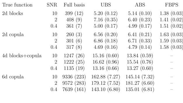
Table 2.1: Means and standard errors (in parentheses) of computational time (in seconds) for four multivariate cases, based on 100 simulation runs. (SNR, signal-to-noise ratio; UBS, uniform basis sampling; ABS, adaptive basis sampling; FBPS, fast bivariate P-splines.)
True function SNR Full basis UBS ABS FBPS
2d blocks 10 399 (12) 5.20 (0.12) 5.14 (0.10) 1.38 (0.03) 2 408 (9) 7.16 (0.35) 6.40 (0.23) 1.41 (0.02) 0.4 361 (7) 5.00 (0.17) 4.99 (0.17) 1.51 (0.02) 2d copula 10 260 (3) 6.56 (0.20) 6.41 (0.21) 1.63 (0.03) 2 301 (6) 6.86 (0.18) 6.71 (0.33) 1.59 (0.03) 0.4 317 (8) 4.69 (0.16) 4.79 (0.14) 1.58 (0.03) 4d blocks+copula 10 1247 (26) 15.16 (0.60) 13.84 (0.59) – 2 1222 (25) 16.62 (0.96) 15.54 (0.76) – 0.4 1135 (19) 13.16 (0.66) 13.27 (0.60) – 6d copula 10 9336 (223) 162.88 (7.27) 145.14 (7.32) – 2 9572 (283) 179.12 (7.52) 181.27 (6.60) – 0.4 7639 (161) 143.10 (6.80) 135.01 (6.81) –
Table 2.1 summarizes the CPU times of all methods based on 100 runs using Intel Xeon 2.90GHz processor with 64GB of DDR3 RAM. The computing time for the full basis smoothing spline estimator is tens or hundreds times more than that for the basis sampling methods, and for the bivariate cases, the fast bivariate P-spline is the fastest in computation.
2.6 Real data example
At a depth of 2890 km in the Earth, the core-mantle boundary separates turbu-lent flow of liquid metals in the outer core from slowly convecting, highly viscous mantle silicates. The core-mantle boundary marks the most dramatic change in dy-namic processes and material properties in our planet, and accurate images of the structure at or near it over large regions are important for our understanding of the geodynamical processes and the thermo-chemical structure of the mantle and mantle-core system.
To accurately image the core-mantle boundary region, Wang et al. (2006) and Ma et al. (2007) developed a generalized Radon transform to construct raw point images, and applied the smoothing spline method to the raw images. In particu-lar, they extracted seismic waves reflected at core-mantle boundary regions from the public data management center of the Incorporated Research Institutions for Seis-mology. The seismic waves extracted were generated by around 1300 earthquakes with magnitude mb >5.2 that occurred between 1988 and 2002, and were recorded at one or more of a total of nearly 1200 stations in central America. Along a 2500 km strip, they then constructed point images of core-mantle boundary regions using a generalized Radon transform. They constructed 163,713 point images at various depths and locations of the strip. At each depth and location, the point images constructed contain many noisy replicates resulting from different reflection angles of the seismic waves, so further statistical analysis is necessary to estimate the true image. In order to be computationally feasible, they estimated the true image using smoothing splines at each location and interpolated the estimated images from all lo-cations to get the three-dimensional image. The image shows peaks of very different magnitudes at several unexpected locations (van der Hilst et al., 2007).
In this section, we apply a smoothing spline with adaptive basis sampling directly to all point images to estimate the three-dimensional image. We let yij denote the
point image at the ith distance, xh1i, and the jth depth, xh2i. We consider the following model for the point images
yij =η(xh1ii, xh2ij) +ij.
Since the sample size is n = 163,713, the regular tensor product smoothing spline is computationally prohibitive. Instead, we apply our cubic tensor product smoothing spline with adaptive basis sampling to the data set with K = 10 slices and let the dimension of the effective model space be n∗ = 155. Define k1(u) =u−0.5,
k2(x) = 1 2{k 2 1(x)− 1 12}, k4(x) = 1 24{k 4 1(x)− k2 1(x) 2 + 7 240},
and R(u1, u2) = k2(u1)k2(u2)−k4(|u1−u2|). The cubic tensor product smoothing spline estimator with adaptive basis sampling has the form
η(x) = 4 X ν=1 dνφν(x) + n∗ X j=1 cjRJ(x∗j, x),
where φ1(x) = 1, φ2(x) = k1(xh1i), φ3(x) =k1(xh2i), φ4(x) = k1(xh1i)k1(xh2i) and
RJ(x, y) =θ1R(xh1i, yh1i) +θ2R(xh2i, yh2i)
+θ3R(xh1i, yh1i)k1(xh2i)k1(yh2i) +θ4R(xh2i, yh2i)k1(xh1i)k1(yh1i) +θ5R(xh1i, yh1i)R(xh2i, yh2i).
The contour plot of the estimated image is provided in Figure 2.4. There, we set the depth of core-mantle boundary (2890 km) as coordinate zero for depth. We can
−30 −20 −10 0 10 20 30 40 500 1000 1500 2000 −200 −100 CMB 100 200 300 400 Distance (km) Depth (km)
Figure 2.4: The estimated image of core-mantle boundary (CMB) region structure using smoothing spline with adaptive basis sampling.
clearly see a peak at depth zero at all distances, which reveals that the core-mantle boundary is a major boundary. It is interesting that we see two disconnected peaks in the depth around 200 km above the core-mantle boundary: one is below and the other is above. We also calculated 95% Bayesian confidence intervals and found them to indicate that these peaks are significantly nonzero. These structures are likely to be the so-calledD00 region, and have also been detected using nonparametric mixed-effect models developed in van der Hilst et al. (2007).
3. REGRESSION WITH RESPONSES FROM EXPONENTIAL FAMILIES
3.1 Introduction
With the rapid development of biotechnologies, second-generation sequencing technologies have become default methods for various genomic and epigenomics anal-ysis, i.e., RNA-seq for gene expression analysis (Mortazavi et al., 2008; Wilhelm et al., 2008; Nagalakshmi et al., 2008), bisulfite sequencing for DNA methylation analysis (Cokus et al., 2008; Lister et al., 2008), and ChIP-seq for genome-wide protein-DNA interaction analysis (Boyer et al., 2005; Johnson et al., 2007; Dixon et al., 2012). Compared to their hybridization-based counterparts, e.g., microarry and ChIP-chip, second generation sequencing technologies offer up to a single-nucleotide resolution signals. In particular, these second-generation sequencing technologies sequence tens of millions of DNA or cDNA fragments in parallel. After mapping the resulting se-quences (short reads) to reference genome, researchers get a sequence of read counts. That is, at each nucleotide position, researchers get a count which stands for the number of reads mapped onto that position. By design, these short read counts reflect the quantity of interests. Statistical modeling and inference are indispensable for analyzing the short read counts to facilitate biological discoveries (Li et al., 2010; Ji et al., 2014). Moreover, as the second-generation sequencing technologies become mature and cost-effective, conducting experiments with samples at multiple condi-tions, and/or of multiple tissue types, and/or at different time points is becoming very common. Since each sequencing sample provides a genome size data, multiple samples give rise to to data of size in tens of millions. The computation of many statistical methods are infeasible to such large sample data. Denote the ith read count by Yi, which associates with some covariates (features)xi, where i= 1, . . . , n.
Two typical examples of research works are given below.
3.1.1 Estimating gene expression in RNA-Seq
In these studies, researchers are interested in measuring the quantities of mR-NAs molecules, i.e., quantifying gene expressions. Since they are more stable and easily degraded, mRNA molecules are shattered and converted into more stable cD-NAs fragments that are short enough suitable for sequencing. The sequenced short fragments are called short reads, which are then aligned to the reference genome to get short-read counts. Finally, gene expressions are estimated based on short-read counts. A simple proposal of estimating gene expression is to average the short-read counts across all nucleotides (within exons) in each gene (normalized by total read counts in the sample) resulting in so-called RPKM (reads per kilobase exon per mil-lion mapped reads) (Cloonan et al., 2008). In this approach, the short-read counts at all nucleotides in a gene are assumed to be a iid sample of a population. How-ever, significant sequencing bias of short-read counts has been observed (Dohm et al., 2008). In particular, short-read counts at a nucleotide position tend to correlate with GC content in the neighborhood of that nucleotide position. Thus appropriate mod-eling the variation of short-read counts within each single gene and the variations among genes across the whole genome is crucial to calculating the gene expressions accurately.
Example 1. Profiling time course gene expression in RNA-Seq. In these studies, gene expressions over a number of time points in a certain biological process are quantified using RNA-seq. After mapping, read counts at each nucleotide position of the whole genome are obtained at each time point. Thus appropriate modeling the variation of short-read counts within each single gene over time while taking into account the GC bias inherited in the RNA-seq technology is crucial to profiling
the gene expressions over the whole time period accurately. In these studies, the response Yi is the short-read count of the ith nucleotide in a gene. Besides time t,
we also have multivariate factor covariate xit = (xhi1ti,· · · , xhiKti), wherexhikti is the GC content in the surrounding k neighborhoods of theith nucleotide in the gene for k = 1, . . . , K. 2
3.1.2 Genome-wide methylation analysis using bisulfite sequencing
DNA methylation is an important epigenetic mechanism that regulates gene ex-pression, cell differentiation and development. It adds a methyl group to a cytosine in CpG dinucleotide (CpG dinucleotide means that a cytosine (C) nucleotide oc-curs next to a guanine (G) nucleotide. The CpG notation is used to distinguish it from the CG base-pairing in DNA double helix). A current technique for measuring DNA methylation levels is bisulfite sequencing. In this technique, DNA is teated with sodium bisulfate, which converts cytosine (C) residues to uracil (U), but leaves methylated cytosine residue unaffected due to the protection of the methyl group. Hence, bisulphite treatment enables changes in the DNA sequence that depend on the methylation status of individual cytosine residues, yielding single nucleotide res-olution information about the methylation status of the DNA sequence (Ji et al., 2014). After sequencing and mapping, the number of short reads mapped onto each CpG site is counted. Thus, bisulfite sequencing data consist of the total number of short reads and methylated reads at each CpG site. Such data allow researchers to estimate methylation proportions at a single-nucleotide resolution.
Example 2. Identifying differentially methylated regions using bisulfite sequencing. In these studies , the methylation levels are measured at two conditions using bisulfite sequencing. The goal is to compare the DNA methylation levels and identify the differentially methylated regions (DMRs). After bisulfite sequencing and mapping,
the number of short reads mapped onto each CpG site is counted. The total number of the mapped reads at the ith position is denoted as Ni, and that of methylated
reads is denoted as Yi. To identify the differentially methylated regions, we have
bivariate covariate xi = (xhi1i, xhi2i) where xhi1i is the genomic location and xhi2i is condition indicator. 2
3.1.3 Exponential family smoothing spline ANOVA models
To provide a rich family of distributions in modeling these data, we assume the conditional distribution ofYi given some covariatexi has a density in the exponential
family with the form
f(Yi|xi) = exp{(Yiη(xi)−b(η(xi)))/a(φ) +c(Yi, φ)}, (3.1)
where i = 1,· · · , n, a > 0, b and c are known functions, η(x) is the regression function to be estimated, and φ is the dispersion parameter, which is assumed to be a constant, either known or considered as a nuisance parameter. Exponential family includes binomial, Poisson, negative binomial, and log normal distributions in a unified framework and is broad enough to cover all practical applications in second-generation sequencing data.
The short-read counts and their derived data from second-generation sequencing techniques are often in drastically different magnitudes at different genomic positions. Versatile nonparametric modeling ofη(xi) in (3.1) provides satisfactory
goodness-of-fit (Zheng et al., 2011; Jaffe et al., 2012). Smoothing splines have been primarily employed as simple smoothing tool to remove noise along genomic positions for single sequencing sample (Kuan et al., 2011; Hansen et al., 2012). When one has sequencing data from two treatment groups as in Example 2, smoothing splines may be applied to short read counts of each individual sample separately to get smoothed profiles
along genome positions. Additional models and methods are then applied to the smoothed sequencing profile to extract signal of interest. In principal, such goal can be achieved through an integrated model and inference strategy via analysis of variance through smoothing spline ANOVA (Gu, 2013).
However, the wide application of smoothing spline ANOVA models in modeling second-generation sequencing data has been hindered due to its expensive compu-tational cost, which is O(n3) where n is sample size. Since the sample size of the second-generation sequencing data is in tens of millions, the computation cost of smoothing spline ANOVA estimates for multivariate x in such super-large samples is prohibitively expensive. Numerous solutions have been proposed in the literature to address the computational issue. For example, hybrid adaptive splines (Luo and Wahba, 1997) integrate a stepwise approach to select nodes and then use the reduced set of nodes to approximate full basis smoothing spline ANOVA models. However, the stepwise nodes selectionper seis computational expensive. The regression splines (Ruppert et al., 2003) take the advantage of closed form solution of smoothing splines and use a small number of nodes to reduce computational cost. The downside of the method is that nodes placement, in general, needs manually conducted, which is in-feasible for genome scale second-generation sequencing data. A recent development along this line of thinking is to use randomly allocated nodes (Gu and Kim, 2002). Albeit it is much simple to implement and faster to compute, the method tends to provide over-smoothed estimates when applied to second-generation sequencing data, and consequently, fails to detect subtle signals.
To surmount these challenges, we develop an adaptive basis selection method for approximating smoothing spline ANOVA models in the exponential family to model second-generation sequencing data. In the proposed method, we evaluate smoothing spline ANOVA models in a lower dimensional effective model space. We construct
the effective model space through an adaptive sampling method via slicing the range of the read counts or the derived data. The sampling strategy and lower effective model space give rise to a more scalable computation for approximating smoothing spline ANOVA models to super-large data, whereas slicing the response provides a representative set of basis functions corresponding different magnitudes of response. The proposed method distinguishes itself from the uniform subsampling approach in selecting smoothing spline basis functions on the direction of the predictors, e.g., Gu and Kim (2002). As evident in our simulation and real data analysis studies, smooth-ing spline ANOVA models approximation via adaptive basis selection provide very accurate estimates. Our symptomatic theory is nonstandard because of the response-dependent sampling scheme. Our asymptotic functional eigenvalue analysis shows the effective model space is rich enough to retain the essential information of true re-gression functions and smoothing spline ANOVA models via adaptive basis selection converge at the same convergence rate of regular smoothing spline ANOVA models. Moreover, our theory provides a practical guidelines for choosing the dimension of the effective model space.
The remainder of the chapter is organized as follows. In Section 3.2, we develop the smoothing spline ANOVA via adaptive basis selection method. The asymptotic analysis is presented in Section 3.3. Simulation and real data analysis follow in Sections 3.4 and 3.5. A few remarks in Section 3.6 conclude the chapter. Proofs of the theorems are collected in Chapter 4.
3.2 Efficient computation of smoothing spline ANOVA models via adaptive basis selection
In this section, we first review the penalized likelihood method for fitting smooth-ing spline ANOVA models and investigate the computation complexity, then develop
the adaptive basis selection method to efficiently approximate the estimator in a low dimensional function space.
3.2.1 Penalized likelihood for fitting smoothing spline ANOVA models
We estimateη by minimizing the penalized likelihood functional
−1 n n X i=1 {Yiη(xi)−b(η(xi))}+ λ 2J(η), (3.2)
where the first term is derived from the negative log likelihood, and J(η) = J(η, η) is a quadratic functional penalizing the roughness ofη. Whenηis a univariate function, a typical choice of J is J(η) = R(η00)2. Other examples of J are given at the end of this subsection. The smoothing parameter λ then controls the trade-off between the goodness-of-fit and smoothness of η.
According to (3.1) we can make distribution assumptions in the afore-mentioned examples.
Example 1 (continued) Profiling time course gene expressions in RNA-Seq. We assume the short-read countY given the covariatexis Poisson distributed, i.e.,Y|x∼ Poisson(λ(x)) with density λ(x)Ye−λ(x)/Y!. This is a special case of exponential family density (3.1) withη(x) = logλ(x),a(φ) = 1,b(η) =eη andc(Y, φ) =−logY!. The Poisson intensity λ(x) is not to be confused with the smoothing parameter λ appearing in (3.2). Besides Poisson distribution, Sun et al. (2015) models the read countY by a negative binomial distribution to account for excessive variation in read counts. In particular,Y|x∼NBinomial(r, p(x)) with density Y+Yr−1p(x)Y(1−p(x))r
such that η(x) = logp(x), a(φ) = 1, b(η) =−rlog(1−eη) and c(Y, φ) = log Y+r−1
Y
as in (3.1). 2
the number of methylated reads Y given covariate x at position is binomial dis-tributed, i.e., Y|x ∼Binomial(N, p(x)) with density NY
p(x)Y(1−p(x))N−Y.
Com-pared with (3.1), η(x) = log{p(x)/(1−p(x))}, a(φ) = 1, b(η) = Nlog(1 +eη) and
c(Y, φ) = log NY. 2
Usually the quadratic functional J(η) is a square semi-norm and the standard formulation of smoothing splines restricts minimizing (3.2) in a reproducing kernel Hilbert space (RKHS) H = {η : J(η) < ∞}. A Hilbert space has a metric and a geometry that facilitate analysis and computation. To prevent interpolation, the null space of J, NJ = {η : J(η) = 0}, is assumed to be a finite dimensional linear
subspace of H with basis {φi: i= 1,· · · , m}. Denote the orthogonal decomposition
of H byNJ ⊕ HJ whereHJ is still a reproducing kernel Hilbert space. Let RJ(x, y)
be the reproducing kernel ofHJ. The representer theorem (Wahba, 1990) shows that
the minimizer of (3.2) in the RKHS H have a simple form
η(x) = m X ν=1 dνφν(x) + n X i=1 ciRJ(xi, x), (3.3)
where coefficients dν and ci are to be estimated from data.
For multivariate x, the smoothing spline analysis of variance (ANOVA) decom-position of a multivariate function η is
η(x) =η0+ d X j=1 ηj(xhji) + d X j=1 d X k=j+1 ηjk(xhji, xhki) +. . .+η1,...,d(xh1i, . . . , xhdi) (3.4)
where the η0 is a constant, theηj’s are the main effects, theηjk’s are the two-way
in-teractions, etc. The identifiability of the terms in (3.4) is ensured by side conditions through averaging operators (Wahba, 1990; Gu, 2013). To use (3.4) for estimat-ing η in (3.2) , we consider ηj ∈ Hhji, where Hhji is an RKHS with tensor sum
decomposition Hhji =H0hji⊕ H1hji, where H0hji is the finite-dimensional “paramet-ric” subspace consisting of parametric functions, and H1hji is the “nonparametric” subspace consisting of smooth functions. The induced tensor product space is
H =⊗dj=1Hhji =⊕S[(⊗j∈SH1hji)⊗(⊗j /∈SH0hji)] =⊕SHS,
where the summation runs over all subsets S ⊆ {1, . . . , d}. The corresponding penalty function J(η) = P
Sθ −1
S JS(ηS) with ηS ∈ HS, θS > 0 are extra smoothing parameters, and JS is the square norm in HS. The subspaces HS form two large subspaces: NJ = {η : J(η) = 0}, which is the null space of J(η), and H NJ with
the reproducing kernel RJ = P
SθSRS where RS is the reproducing kernel in HS. The smoothing spline estimator in such reproducing kernel Hilbert space is called a tensor product smoothing spline.
Example 1 (continued) Profiling time course gene expressions in RNA-Seq. In the functional ANOVA decomposition of η(x), exp{η0} denotes time course gene expression level, all other main effects and interactions are sequencing bias need to be removed. 2
Example 2 (continued) Identifying differentially methylated regions. Applying function ANOVA to η, we can identify significantly different methyaltion profiles over two conditions. 2
In Example 2, we encounter the case where covariates are of mixed types. Con-sider a bivariate functionη(x, τ), wherex∈[0,1] andτ ∈ {1, . . . , t}. A valid decom-position isη(x, τ) =η∅+η1(x) +η2(τ) +η1,2(x, τ),where η∅ is a constant, η1(x) is a function ofx satisfying η1(0) = 0,η2(τ) is a function ofτ satisfying
Pt
τ=1η2(τ) = 0, and η1,2(x, τ) satisfies η1,2(0, τ) = 0, ∀τ, and
Pt
quadratic functional J, one may use J(η) =θ−11 Z 1 0 (d2η1/dx2)2dx+θ−11,2 Z 1 0 t X τ=1 (d2η1,2/dx2)2dx.
The null space NJ has dimension 2t with basis given by
{1, x, I[τ=j]−1/t,(I[τ=j]−1/t)x, j = 1, . . . , t−1}.
Moreover, the reproducing kernel of HJ is
RJ(x1, τ1;x2, τ2) = θ1
Z a
0
(x1−u)+(x2−u)+du+θ1,2(I[τ1=τ2]−1/t) Z a
0
(x1−u)+(x2−u)+du.
General discussion can be found in Chapter 2.4 of Gu (2013).
By standard exponential family theory, E[Y|x] =b0(η(x)) =µ(x) and var[Y|x] = b00(η(x))a(φ) =ν(x)a(φ). When the likelihood function in model (3.2) has a unique minimizer in NJ, the minimizer ˆη of (3.2) uniquely exists. Fixing the smoothing
parameter λ (and ones hidden in J(η), if present), (3.2) may be minimized through the Newton iteration. Write l(η(xi);Yi) =−Yiη(xi) +b(η(xi)), u(η(xi);Yi) =−Yi+
b0(η(xi)), and w(η(xi);Yi) = b00(η(xi)) = ν(xi). The quadratic approximation of
l(η(xi);Yi) at the current estimate ˜η(xi) is seen to be
l(η(xi;Yi)≈l(˜η(xi);Yi)+˜ui(η(xi)−˜η(xi))+ ˜wi(η(xi)−˜η(xi))2/2 = ˜wi( ˜Yi−η(xi))2/2+Ci,
where ˜ui =u(˜η(xi);Yi), ˜wi =w(˜η(xi);Yi), ˜Yi = ˜η(xi)−u˜i/w˜i and Ci is independent
of η(xi). The Newton iteration can thus be performed to penalized weighted least
squares, n X i=1 ˜ wi( ˜Yi−η(xi))2+nλJ(η). (3.5)
Although fast algorithms (Reinsch, 1967) are available whenx is univariate, the computation of (3.5) for multivariate x is at least in the order of O(n3), see Chap-ter 3.4 of Gu (2013). The high computational cost of smoothing splines render its inapplicability in modeling second-generation sequencing data. In our examples, sample sizes are 48,660 and 23,361.
3.2.2 Adaptive basis selection
To alleviate computational cost of smoothing splines, one may restrict the min-imizer of (3.2), equivalently (3.5), in a reduced subspace of H. Such subspace is called an effective model space with two distinguishing features. First, the computa-tional cost in constructing the effective model space is very inexpensive; second, the effective model space retains the essential information of the true functionη. Gu and Kim (2002) and Kim and Gu (2004) developed a simple random sampling approach to select a subset of full basis functions and construct an effective model space. The resulted estimator shares the same asymptotic convergence rates with the estimator constructed with full basis functions. Following this idea, we propose an adaptive basis selection algorithm to construct the effective model space. The intuition is to first produce a crude estimate of the conditional density f(x|y) using a simple slicing technique and then guarantee the most influential basis functions included in the effective model space. In particular, when the underlying function varies signif-icantly in magnitude, the estimates based on such adaptive sampling approach will outperform the the estimates based on uniform random sampling.
Adaptive basis selection algorithm
(1) Divide the range of the responses {Yi}ni=1 into a number of disjoint intervals,
(2) For k = 1, . . . , K, take a random sample x∗(1k), . . . , x∗(nkk) of size nk without
re-placement, from original sample xi with probability |Sk|−1Iyi∈Sk, where |Sk|
is the number of observations in Sk. We denote the combined sample as
x∗1, . . . , x∗n∗ with sample size n∗.
(3) Finally, minimizing criterion (3.2) over
HE =NJ⊕span{RJ(x∗j,·), j = 1, . . . , n
∗}
where HE is referred to as the effective model space. The minimizer then has the expression ˆ ηA(x) = m X i=1 dνφν(x) + n∗ X j=1 cjRJ(x∗j, x) (3.6) where ηˆA(x) is a smoothing spline ANOVA estimate through adaptive basis selection.
When dividing the range of response variable, we need take the specific exponen-tial family into account. In Example 1, responses follow a Poisson distribution and we can apply step (1) directly. However, in Example 2 where Yi follows a binomial
distribution, we instead propose t