observations of a diffusion process
Benjamin Favetto
To cite this version:
Benjamin Favetto. Parameter estimation by contrast minimization for noisy observations of a diffusion process. MAP5 2010-13. 2010. <hal-00493967v2>
HAL Id: hal-00493967
https://hal.archives-ouvertes.fr/hal-00493967v2
Submitted on 31 Dec 2012HAL is a multi-disciplinary open access archive for the deposit and dissemination of sci-entific research documents, whether they are pub-lished or not. The documents may come from teaching and research institutions in France or abroad, or from public or private research centers.
L’archive ouverte pluridisciplinaire HAL, est destin´ee au d´epˆot et `a la diffusion de documents scientifiques de niveau recherche, publi´es ou non, ´emanant des ´etablissements d’enseignement et de recherche fran¸cais ou ´etrangers, des laboratoires publics ou priv´es.
Statistics
Vol. 00, No. 00, December 2011, 1–29
ARTICLE
Parameter estimation by contrast minimization for noisy
observations of a diffusion process
Benjamin Favettoa∗ aUniversit´e Paris Descartes
(v2 released November 2012)
We consider the estimation of unknown parameters in the drift and diffusion coefficients of a one-dimensional ergodic diffusionX when the observationY is a discrete sampling ofX
with an additive noise, at timesiδ, i= 1. . . N. Assuming that the sampling interval tends to 0 while the total length time interval tends to infinity, we prove limit theorems for functionals associated with the observations, based on local means of the sample. We apply these results to obtain a contrast function. The associated minimum contrast estimators are shown to be consistent. Some examples are discussed with numerical simulations.
Keywords:contrast function; diffusion process; hidden Markov models; parametric inference; discrete time noisy observations
AMS Subject Classification: 62M09; 62F12
1. Introduction
Statistical inference for continuous time models based on high frequency data has been the subject of a huge number of recent papers. On one hand, continuous time stochastic processes are increasingly used for modelling purposes. On the other hand, such kind of data is now commonly available in various fields of applications whether in finance or in biology and medicine.
Among continuous time models, one-dimensional diffusion processes have re-ceived a lot of attention. More precisely, let (Xt) be given by the stochastic differ-ential equation:
dXt=b(Xt, κ)dt+σ(Xt, λ)dBt, X0 =η (1)
withB a standard Wiener process andηa random variable independent ofB, and
b(., κ), σ(., λ) real valued functions, defined on R, depending on unknown param-eters (κ, λ) ∈Rd1 ×Rd2. The estimation of θ= (κ, λ) based on a discrete sample
(Xiδ, i ≤ N) with small sampling interval δ has been largely investigated. (see
e.g.[6], [7] for contrast-based estimator of the drift parameter, [22]for maximum likelihood estimator, [8] for the estimation of the diffusion coefficient of multidi-mensional diffusion process, [16] for the case of an ergodic diffusion observed on a long-time interval, [2], [21], [1] . . . )
∗Email: [email protected]
ISSN: 0233-1888 print/ISSN 1029-4910 online c
2011 Taylor & Francis
DOI: 10.1080/0233188YYxxxxxxxx http://www.informaworld.com
In this paper, we suppose that, instead of observing exactlyXiδ, the observation at timeiδ is given by
Yiδ=Xiδ+ρεiδ (2)
with (εiδ, i ≥ 0) a sequence of i.i.d. random variables, satisfying E(εiδ) = 0, E((εiδ)2) = 1, independent of the process (Xt). This kind of model takes into account measurement errors or, in the case of financial data, the so-called mi-crostructure noise. In this context, the estimation of the integrated volatility has been widely investigated (seee.g[23]). Jacodet al. in [15] consider the same kind of observations for δ =δN, over an interval of lengthN δN =t fixed, to estimate
the integrated volatilityR0tσ(Xs, λ)2ds.
From now on, our concern is the joint estimation of θ = (κ, λ) using discrete observations 2 over a long-time interval.
The exact likelihood of (Yiδ, i ≤ N) given by (1)-(2) is generally intractable except for few models (essentially for Gaussian diffusions with additive Gaus-sian noise, see e.g. [3], [17], [5]). For data within a fixed length-time interval (δ=δN = N1,N δN = 1), estimation for a general diffusion with additive Gaussian noise is investigated in [12]. The authors use a contrast method and only diffusion coefficient parameters can be consistently estimated in this case. For the nonpara-metric case, the inference of the drift function and the diffusion coefficient have been studied in [20] and [19].
In this paper, we study observations given by (1)-(2) where δ =δN → 0 while
N δN → ∞, under ergodic properties for the hidden diffusionX and propose con-sistent estimators of both the drift and diffusion coefficient parameters (κ, λ). The noise distribution is unknown, the varianceρ2 of the noise term may be known or unknown and we assume thatρ is fixed.
Our starting idea is to reduce the influence of the noise by splitting the sample into sub-samples and taking empirical means of the sub-samples. More precisely, the sample is split intok blocks of sizep, withN =pk, wherep=pN and k=kN tend to infinity withN. Then, setting ∆N =pNδN where pN and δN are chosen such that ∆N →0, we build the empirical mean of thejth block:
Y•j =X•j+ρεj•, j= 0,1. . . kN −1, (3) where, forZ =Y, X, ε, Z•j = 1 pN pN−1 X i=0 Zj∆N+iδN. (4)
Thus, ∆N defines a coarser sampling interval than δN, still tending to 0 while
N δN =kN∆N → ∞.
Our statistical procedure is based on the kN− sample (Y•j, j = 0. . . kN −1) and follows a scheme analogous to the one in [11]. Hence, the empirical mean
X•j = p1N Ppi=0N−1Xj∆N+iδN of the diffusion is closed to the integrated process
1 ∆N
R(j+1)∆N
j∆N XsdsasδN is sufficiently small. The parameter estimation ofκandλ
based of the observations of an integrated diffusion process has been investigated by Gloter in [9], [10] and [11]. Our approach is based on these considerations.
We study the differences Y•j −Xj∆N (Proposition 3.2) and prove a regression
type relation for the Y•j’s (Proposition 3.4) which is the base of the statistical
the quadratic variation of (Y•j) which hold by setting δN = p−Nα with 1 < α ≤ 2 (Theorems 4.2 and 4.3). We introduce contrasts and prove the consistency of the associated minimum contrast estimators. The study of the asymptotic distributions of the minimum contrast estimators is studied in another paper, as it requires further developments (see [4]).
The paper is organised as follows. In Section 2, notations and assumptions on the model are precised. Section 3 is devoted to the small sample properties of the empirical means sample (Y•j) and Section 4 to uniform convergence in probability
results. In Section 5, we introduce the contrasts and prove the consistency of the estimators. We also deal with the caseρunknown and prove thatρ2can be replaced by an estimator in the contrast formula. Section 6 is devoted to examples and numerical results. For several models, we implement our estimators on simulated data for different choices of (N, δN, pN) and of the noise level. Section 7 contains some concluding remarks. Proofs are gathered in Section 8, and some auxiliary results are recalled in the Appendix.
2. Assumptions and Notations
Consider the one-dimensional stochastic differential equation
dXt=b(Xt, κ0)dt+σ(Xt, λ0)dBt, X0 =η (5)
where B is a standard Brownian motion and η is a real valued random variable independent of B. The functions b(x, κ) and σ(x, λ) are respectively defined on R×Θ1 and R×Θ2 where Θ1 (resp. Θ2) is a compact convex subset of Rd1 (resp.
Rd2). For simplicity of notations, in proofs, we assume thatd
1 =d2 = 1. We denote
by θ0 = (κ0, λ0) the true value of the parameter and assume that θ0 ∈
◦
Θ where Θ = Θ1×Θ2.
From now on, we set b(x) =b(x, κ0) and σ(x) =σ(x, λ0) and make classical
as-sumptions on functionsbandσensuring that (5) admits an unique strong solution (Xt)t≥0, defined on a probability space (Ω,F,P), and that this solution is positive
recurrent onR.
(A1) Functions b and σ belong to C2(R), σ(x) >0 for all x, and there exists c > 0
such that for all x∈R:
|b(x)|+|b0(x)|+|b00(x)| ≤c(1 +|x|), σ(x) +|σ0(x)|+|σ00(x)| ≤c(1 +|x|).
(A2) For x0 ∈ R, let s(x) = exp(−2
Rx
x0
b(u)
σ2(u)du) denote the scale density and m(x) = σ2(x1)s(x) the speed density. Assume
R
−∞s(x)dx =
R+∞
s(x)dx = ∞
and R−∞+∞m(x)dx=M <∞.
(A3) Letν0(dx) = M1 m(x)dx. For all k >0, ν0 admits a finite moment of order k. (A4) For allk >0,supt≥0E(|Xt|k)<∞.
(A5) The common distribution of the random variables εiδN admits a 8th order
mo-ment, and is symmetric.
Assumption(A1) implies that (1) admits a unique strong solution on R. Under
classical ergodic theorem (seee.g.[18]) ∀f ∈L1(dν0), 1 T Z T 0 f(Xs)ds −→ T→∞ν0(f) a.s.
Moreover, under Assumption(A1), for all k≥1, there exists a constantc(k)such that, for allt≥0:
E sup s∈[t,t+1] |Xs|k Gt ! ≤c(k)(1 +|Xt|k). (6)
where Gt = σ(Bs, s ≤ t;η). (See e.g [9]). Furthermore, Assumptions (A1)-(A3) imply(A4) if η has distribution ν0 or η is deterministic (for the latter case, see
[11], Proposition 3). Below, we first assume that the noise level ρ is known and discuss later the case whereρ is unknown.
Define the σ-fields
GN
j =Gj∆N =σ(Bs, s≤j∆N;η), HNj =GjN ∨ ANj ,
AN
j =σ(εk∆N+iδN, i≤pN −1, k≤j−1) =σ(εlδN, l≤j∆N −δN)
(7)
For 0 ≤j ≤kN −1, the random variable Y•j is HNj+1 measurable. We introduce,
for further use, a condition on functionsg:R×Θ−→R:
(C1) The functiong is the restriction of a function defined onR× Owith Oan open neighbourhood of Θ and
∃c >0,∀x∈R sup θ∈Θ
|g(x, θ)| ≤c(1 +|x|).
We need the following statistical assumptions ((A6) is the usual identifiability condition for this problem and(A7)is a smoothness condition for the contrast):
(A6)
σ(x, λ) =σ(x, λ0) ν0 almost everywhere impliesλ=λ0,
b(x, κ) =b(x, κ0) ν0 almost everywhere impliesκ=κ0.
(A7) The partial derivatives∂xb,∂κb,∂xσ,∂λσ,∂xx2 b,∂κκ2 b,∂xκ2 b,∂xxσ,∂λλ2 σand∂xλ2 σ exist, are continuous and satisfy Condition (C1).
3. Small sample properties of the local means sample
In this section, some local properties of the local means are gathered ton enlight first order approximation ofY•j−Xj∆N and Y•j+1−Y•j.
The following random variables appear in the expansions below:
ζj+1,N = 1 pN pN−1 X i=0 Z (j+1)∆N j∆N+iδN dBs, ζj0+2,N = 1 pN pN−1 X i=0 Z (j+1)∆N+iδN (j+1)∆N dBs, (8)
ex-pansions: ξj0+1,N = 1 ∆3N/2 Z (j+2)∆N (j+1)∆N ((j+ 2)∆N −s)dBs, (9) ξ0i+1,j,N = 1 δN3/2 Z j∆N+(i+2)δN j∆N+(i+1)δN (j∆N+ (i+ 2)δN−s)dBs. (10)
Some basic properties of these random variables are summarized in Lemma 8.1 and in Lemma 8.2 in Section 8.
Proposition 3.1 : Let X¯j = ∆−N1
R(j+1)∆N
j∆N Xsds. Under Assumption (A1), we
have ¯ Xj−X•j = p δN 1 pN pN−1 X i=0 σ(Xj∆N+iδN)ξ 0 i,j,N ! +ej,N with (see (7)) ∃c >0, |E(ej,N|HNj )| ≤δNc(1 +|Xj∆N|), E(e2j,N|HNj )≤δN2c(1 +|Xj∆N|4).
The following proposition precises the local asymptotic behaviour of the observa-tion blocks, by a first order comparison betweenY•j andXj∆N. It can be compared
to Proposition 2.2 in [9].
Proposition 3.2 : Under (A1), we have for j≤kN−1,
Y•j−Xj∆N =σ(Xj∆N) p ∆Nξj,N0 +e0j,N+ρεj• (11) with|E(e0j,N|HN j )| ≤c∆N(1 +|Xj∆N|) and E(e0j,N2|HN j )≤c∆2N(1 +|Xj∆N|4), E(e0j,N 4|HN j )≤c∆3N(1 +|Xj∆N|4).
If moreover (A5) holds, for k≤8,
∃c >0,∀j≤kN−1,E |Y•j −Xj∆N|k H N j ≤c∆k/N2(1 +|Xj∆N|k) +ρkE |εj•|k. (12) We deduce:
Corollary 3.3 : Assume (A1) and (A5), and consider f : R2 ×Θ → R such
thatf, ∂xf, ∂xx2 f satisfy (C1). Then
∃c >0,∀j ≥0,∀θ∈Θ, E f(Y•j, θ)−f(Xj∆N, θ) H N j ≤c(∆N(1 +|Xj∆N| 2) +ρ2qE((εj •)4)) (13) and for l= 1,2 E(f(Y•j, θ)−f(Xj∆N, θ))2l H N j ≤c(1 +|Xj∆N|2l+ρ2lE((εj•)2l)) ×(∆lN(1 +|Xj∆N|2l) +ρ2l q E((εj•)4l)). (14)
The following proposition is essential for the limit theorems of Section 4 and for the statistical application.
Proposition 3.4 : Under Assumptions (A1) and (A5), we have
Y•j+1−Y•j−∆Nb(Y•j) =σ(Xj∆N)(ζj+1,N +ζj0+2,N) +τj,N +ρ(εj•+1−εj•)
whereτj,N isHNj+2 mesurable, and there exists a constantc >0 such that
|E(τj,N|HNj )| ≤c∆N(∆N(1 +|Xj∆N|3) +ρ2 q E((εj•)4)), E(τj,N2 |HNj ) +|E(τj,Nζj+1,N|HjN)|+|E(τj,Nζj0+2,N|HNj )| ≤ c∆N(1 +|Xj∆N|2+ρ2E((εj•)2))(∆N(1 +|Xj∆N|4) +ρ2 q E((εj•)4)), E(τj,N4 |HNj )≤c(1 +|Xj∆N|4+ρ4E((εj•)4))(∆4N(1 +|Xj∆N|4) +ρ4 q E((εj•)8)).
Note that, for i= 1,2, by the Rosenthal inequalityρ2i
q E((εj•)4i) =O(ρ 2i pi N ).
3.0.0.1. Remark: . In [9], Theorem 2.3., it is proved that
¯
Xj+1−X¯j−∆Nb( ¯Xj) =
p
∆Nσ(Xj∆N)(ξj,N +ξ0j+1,N) + ¯τj,N
where ¯τj,N satisfies|E(¯τj,N|GjN)| ≤c∆2N(1 +|Xj∆N|3). In Proposition 3.4,
addition-nal terms due to the noise appear.
4. Uniform convergence in probability results
In this section, asymptotic results for functionals of local means are stated. They are involved in the asymptotic study of the minimum contrast estimators described in Section 5.
From now on, f : R × Θ → R denotes a C2 function, such that f, ∂
xf,
∂2
xxf and ∂θf satisfy (C1). The assumptions on asymptotics are denoted (AH) :
(AH) The number of observations N → ∞, with δN → 0, pN → ∞, kN → ∞, ∆N =pNδN →0and N δN =kN∆N → ∞.
The first result is an ergodic theorem for the local means.
Proposition 4.1 : Under Assumptions (A1)-(A5) and (AH), we have
¯ νN(f(., θ)) = 1 kN kN−1 X j=0 f(Y•j, θ)−→ν0(f(., θ)) (15) uniformly in θ, in probability.
Theorem 4.2 : Under Assumptions(A1)-(A5) and(AH), withδN =p−Nα, α∈ (1,2], (∆N =p1N−α) we have ¯ IN(f(., θ)) = 1 kN∆N kN−2 X j=1 f(Y•j−1, θ)(Y•j+1−Y•j −∆Nb(Y•j−1))−→P 0 (16) uniformly in θ.
The late result deals with the quadratic variation of Y•j.
Theorem 4.3 : Assume (A1)-(A5) and (AH). (1) If δN =p−Nα withα∈(1,2)(∆N =p1N−α), then ¯ QN(f(., θ)) = 1 kN∆N kN−2 X j=1 f(Y•j−1, θ)(Y•j+1−Y•j)2 −→P 2 3ν0(f(., θ)σ 2), (17) (2) If δN =p−N2 (∆N = p1N), then ¯ QN(f(., θ))−→P 2 3ν0(f(., θ)σ 2) + 2ρ2ν 0(f(., θ)), (18) uniformly in θ∈Θ.
The proofs of these two last theorems are based on the results of Proposition 3.4 and Lemma A.3 in the Appendix. Theorems 4.2 and 4.3 can be compared tothe following results from [16]:
1 kN∆N kN−1 X j=0 f(Xj∆N, θ)(X(j+1)∆N −Xj∆N −∆Nb(Xj∆N)) =oP(1), (19) 1 kN∆N kN−1 X j=0 f(Xj∆N, θ)(X(j+1)∆N −Xj∆N)2 =ν0(f(., θ)σ2) +oP(1). (20)
Theorem 4.2 gives the analogous result as (19), under the condition δN = p−Nα,
α∈(1,2]and provided that we introduce a lag to avoid correlation terms of order ∆N (if no lag, the limit is not 0, see for instance [11]). Theorem 4.3 underestimates
ν0(f(., θ)σ2)because the variance ofζj+1,N+ζj0+2,N (see Proposition 3.4) is equiv-alent to 23∆N and not to ∆N. ForδN =p−N2, an additional bias appears due to the noise.
5. Estimation by contrast minimization
The main results about minimum contrast estimators using local means are de-scribed here. The contrasts presented in this section are inspired by the works of Kessler (see [16]) and Gloter (see [9] and [11]). They derive from the log-likelihood of independent Gaussian random variables of meanX(j+1)∆N −Xj∆N−
∆Nb(Xj∆N, κ) and variance ∆Nσ
2(X
j∆N, λ) previously used to build a contrast
means (Y•j), mainly justified by the asymptotic behaviour of the quadratic
vari-ation in Theorem 4.3. These constrasts have been modified in [11] to deal with parameter estimation for integrated diffusion processes.
5.1. Definition of the contrasts
Define EN(θ) = kN−2 X j=1 ( 3 2∆N (Y•j+1−Y•j−∆Nb(Y•j−1, κ))2 σ2(Yj−1 • , λ) + log(σ2(Y•j−1, λ)) ) . (21)
WhenδN =p−Nα with α∈(1,2], letcN,ρ(x, λ) =σ2(x, λ) + 3∆
2−α α−1 N ρ2 and define ENρ(θ) = kN−2 X j=1 ( 3 2∆N (Y•j+1−Y•j −∆Nb(Yj −1 • , κ))2 cN,ρ(Y•j−1, λ) + log(cN,ρ(Y•j−1, λ)) ) (22)
We have limN→∞cN,ρ(x, λ) = cρ(x, λ) with cρ(x, λ) = σ2(x, λ) if 1 < α < 2 and
cρ(x, λ) = σ2(x, λ) + 3ρ2 if α = 2. Let ˆθN and ˆθρN be the associated minimum contrast estimators, defined as any solution of
ˆ θN =arginf θ∈Θ EN(θ) and ˆθNρ =arginf θ∈Θ ENρ(θ). (23)
Theorem 5.1 : Assume (A1)-(A7), and consider θˆN and θˆρN defined by (23).
(1) If δN = p−Nα, α ∈ (1,2), the estimator θˆN is consistent: θˆN → θ0 in Pθ0
probability.
(2) If α∈(1,2], the estimatorθˆρN is consistent.
Note that point 1 does not require the knowledge of ρ.
The parameter α links the number of observations pN in a subsample and
the length ∆N in the time-interval of this subsample, as ∆N = pNδN = δ
1−1
α
N .
Tuning α depends on the total number of observations, to deal with a rather large number of observations in each subsample and denoise sufficiently each local mean (See Table 1 in Section 6 for a numerical example).
The limit value α = 2 is determined by the apparition of the variance of the additional noise: there is not enough observations in each subsample to neglectρ2. Hence, the choice of the contrastENρ is motivated by the second result in Theorem 5.1.
5.2. Estimation with unknown observation noise level
Assuming (B1) with unknown ρ, we consider the estimator ρˆ2N =
1 2N
PN−1
i=0 (Y(i+1)δN −YiδN)
2, which is the half of the quadratic variation of the
observations.
Lemma 5.2 : Assume (A1)-(A5) and (B1). Then we have ρˆ2N −→P ρ2, when
N → ∞, with δN →0and N δN → ∞. If, moreover, N δN2 →0,
√
N( ˆρ2N −ρ2)−→L N(0,3ρ4).
The minimum contrast estimator ˆθρˆN
N based on the constrastE
ˆ
ρN
N (θ)satisfies:
Corollary 5.3 : Assume (A1)-(A7), (B1) and δN =pN−α with α ∈(1,2]. The
estimator θˆρˆN
N is consistent.
6. Examples
In this section, simulation results are given for several examples of diffusion models on simulated data.
6.1. Example 1. The Ornstein-Uhlenbeck process
The hidden diffusion solves
dXt=κXtdt+λdBt (24)
withκ <0andλ >0, andX0is deterministic or follows the stationary distribution
ofX. We consider several distributions for the noise.
In this model, we can compute explicitly the estimator ˆθN by minimizing the contrast. With the expressions of∂κEN(θ)and ∂λEN(θ), we find
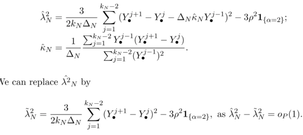
ˆ λ2N = 3 2kN∆N kN−2 X j=1 (Y•j+1−Y•j−∆NκˆNY•j−1)2−3ρ21{α=2}; ˆ κN = 1 ∆N PkN−2 j=1 Y j−1 • (Y•j+1−Y•j) PkN−2 j=1 (Y j−1 • )2 . We can replace ˆλ2 N by ˜ λ2N = 3 2kN∆N kN−2 X j=1 (Y•j+1−Y•j)2−3ρ21{α=2}, as ˆλ2N −λ˜2N =oP(1).
In Tables 1-5, the common distribution of εiδ is N(0,1) and Table 6 presents some results with other distributions. Tables 1, 2 and 3 give mean and variance of ˆθN for different values of δ, α and N (δ = p−α). The values of the parameters are κ0 = −1, λ0 = 1, ρ2 = 0.5. We have used 500 replications, and we give the
empirical mean and variance in parenthesis.
N = 5000, δ= 0.01 (N δ= 50, N δ2= 0.5) κ0=−1, λ0= 1, ρ2= 0.5 α= 1.17(p= 50, k= 100) α= 1.5(p= 22, k= 227) α= 2(p= 10, k= 500) ˆ κN (102 Var) -0.58 (1.53) -0.76 (2.75) -0.82 (3.26) ˆ λ2N (102 Var) 0.76 (1.19) 1.07 (1.25) 0.86 (2.61) Table 1. Influence of the size of blocks on the estimators, Ornstein-Uhlenbeck model.
First, we remark that the empirical variance is larger in the case α = 2than in the other cases. The parameter κ0 is always underestimated, but the estimation
of κ0 is clearly improved as N grows, and δ is close to 0. The estimation of λ0
is better in Table 2 than in Table 1, and similar in Tables 2 and 3. The variance decreases strongly in the caseα= 2.
N = 20000, δ= 0.005 (N δ= 100, N δ2= 0.5) κ 0=−1, λ0= 1, ρ2= 0.5 α= 1.35(p= 50, k= 400) α= 1.5(p= 34, k= 588) α= 2(p= 14, k= 1428) ˆ κN (102 Var) -0.74 (1.08) -0.81 (1.47) -0.87 (1.51) ˆ λ2 N (103 Var) 0.95 (3.87) 1.05 (3.88) 0.92 (11.07) Table 2. Influence of the size of blocks on the estimators, Ornstein-Uhlenbeck model.
N= 100000, δ= 0.001 (N δ= 100, N δ2= 0.1) κ 0=−1, λ0= 1, ρ2= 0.5 α= 1.3(p= 200, k= 500) α= 1.5(p= 100, k= 1000) α= 2(p= 32, k= 3125) ˆ κN (102 Var) -0.81 (1.36) -0.89 (1.49) -0.96 (1.95) ˆ λ2 N (103 Var) 0.90 (2.74) 1.02 (1.99) 0.92 (3.85) Table 3. Influence of the size of blocks on the estimators, Ornstein-Uhlenbeck model.
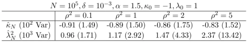
In Table 4, we study the influence of the noise on the estimators, in the case
α = 32. We use 500 replications, with δ = 0.001 and N = 105, and we give the empirical mean and standard deviation in parenthesis.
N = 105, δ= 10−3, α= 1.5, κ0 =−1, λ0 = 1 ρ2 = 0.1 ρ2= 1 ρ2= 2 ρ2 = 5 ˆ κN (102 Var) -0.91 (1.49) -0.89 (1.50) -0.86 (1.75) -0.83 (1.52) ˆ λ2N (103 Var) 0.96 (1.71) 1.17 (2.92) 1.47 (4.33) 2.37 (13.42) Table 4. Influence of the observation noise variance on the estimators, Ornstein-Uhlenbeck model.
A strong bias appears for ˆλN whenρ2is bigger than 1, whereas there are no sig-nificant changes in the estimation of the drift parameterκ0. The empirical variances
for the estimation of λ0 also increases: the presence of noise in the observations
contaminates the estimation of the diffusion coefficient in this case.
In Table 5, we study the influence of the value of the diffusion coefficient on the estimators, in the case α = 32. We use 500 replications, with δ = 0.001 and
N = 105, and we give the empirical mean and variance in parenthesis.
N = 105, δ= 10−3, α= 1.5, κ0=−1, ρ2 = 1 λ20 = 0.1 λ20 = 0.5 λ20= 1 λ20= 2 ˆ κN (102 Var) -0.81 (1.48) -0.87 (1.54) -0.90 (1.64) -0.89 (1.62) ˆ λ2N (103 Var) 0.23 (0.12) 0.58 (0.78) 1.01 (1.95) 2.01 (6.93) Table 5. Influence of the diffusion coefficient on the estimators, Ornstein-Uhlenbeck model.
The smallest value of λ2
0 is overestimated by ˆλ2N, and this result confirms the ones of Table 4 about high levels of noise. For the other values of λ20, no bias is observed.
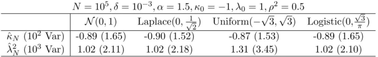
We finally study in Table 6 the influence of the distribution of the errors on the estimators. We choose in this case α = 32, κ0 = −1, λ0 = 1, ρ2 = 0.5 . We use
500 replications, with δ = 0.001 and N = 105, and we give the empirical mean and standard deviation in parenthesis. We make the appropriate corrections on the distributions ofεiδ to have unitary variance.
We observe that, except in the case of a Uniform distribution, the estimators give results close to the Gaussian case. For the case εiδ ∼ Uniform(−
√
3,√3), a significant positive bias is observed, and the variance is larger in this case than in the case of Gaussian distribution.
These simulations point out two facts : first, the value α= 32 for the local mean size parameter appears as a good compromise, with a bias in the estimation of κ
N = 105, δ= 10−3, α= 1.5, κ 0=−1, λ0 = 1, ρ2 = 0.5 N(0,1) Laplace(0,√1 2) Uniform(− √ 3,√3) Logistic(0, √ 3 π ) ˆ κN (102 Var) -0.89 (1.65) -0.90 (1.52) -0.87 (1.53) -0.89 (1.65) ˆ λ2N (103 Var) 1.02 (2.11) 1.02 (2.18) 1.31 (3.45) 1.02 (2.10) Table 6. Influence of the distribution of the noise on the estimation, Ornstein-Uhlenbeck model.
on simulations lower than the variance observed for α = 2. The second remark concerns the number of observations: for N = 5000 observations, κ is underesti-mated, for all the values ofα considered. Thus, the context of high frequency data requires a large number of observations, with a very small discretization step, to be taken into consideration.
6.2. Comparison with a discretely observed Ornstein-Uhlenbeck process
We are interested in the comparison, on simulated datasets, of our method with the methods based on the direct observation of the diffusion at discrete time (see e.g. [7] and [16]). To compare the quality of the noise reduction and its influence on the estimation of the parameters, we compare the results for discrete observations with noise, based on the minimization of the contrast built on the (Y•j) (Tables
1, 2 and 3) with those obtained for the discrete observations without noise, based on the minimization of the contrast built on the (XiδN). In both cases the same
datasets of N observations with a δN-step of discretization are considered. The hidden diffusion (Xt) is an Ornstein-Uhlenbeck process (24). The results based on the direct observations are given in Table 7.
α= 1.5, κ0 =−1, λ0= 1, no noise N = 5.103, δ= 10−2 N = 2.104, δ= 5.10−3 N = 105, δ= 10−3 ˆ κN (Var) -1.04 (0.21) -1.02 (0.13) -1.01 (0.14) ˆ λ2N (Var) 0.99 (1.98×10⁻²) 0.99 (9.80×10⁻³) 1.00 (4.30×10⁻³) Table 7. Parameter estimation with direct observations of the Ornstein-Uhlenbeck model, for several numbers of observations.
The estimation of κ0 is better for a direct observation of the diffusion, but in
this case, the whole set ofN observations is taken into account, whereas the size of the set of local means iskN =N δ
1
α
N.
6.3. Example 2. The Cox-Ingersoll-Ross process
Consider the one-dimensional diffusion process (Cox-Ingersoll-Ross process), solu-tion of
dXt= (κXt+κ0)dt+λ
p
XtdBt, X0=η, (25)
with κ < 0, κ0 ∈R and λ > 0, and η a positive random variable independent of (Bt).
We assume that the observations at time t0 <· · ·< tN are given by
Yti =Xtiexp(εti)
where (εti)is a sequence of independentN(0, ρ
2)random variables. Hence the noise
to have real valued observations. The process Zt = log(Xt) solves the stochastic differential equation dZt= (κ+ (κ0− λ2 2 ) exp(−Zt))dt+λexp(− Zt 2 )dBt. We setκ00=κ0−λ2 2 .
In this case, the scale density iss(x) = exp −2κ λ2e
x−2κ00 λ2 x
and the speed density ism(x) = λ12 exp 2κ00 λ2 + 1 x+2λκ2e x
. Provided κ <0 and 2λκ200 + 1>0,
Assump-tions(A2),(A3)are ensured, and(A4)holds withη ∼ν0. However, Assumption (A1)does not holds, but ˆθN is explicit, and the consistency can be proved directly. Explicit expressions for the estimator ˆθN = (ˆκN,κˆ00N,λˆ2N)are derived: (ˆκN,κˆ00N) is solution of the system
∆NPkj=1N−2exp(Y•j−1) ∆NkN ∆NkN ∆NP kN−2 j=1 exp(−Y j−1 • ) ! ˆ κN ˆ κ00 N = PkN−2 j=1 exp(Y j−1 • )(Y•j+1−Y•j) PkN−2 j=1 (Y j+1 • −Y•j) ! and ˆ λ2N = 3 2kN∆N kN−2 X j=1 exp(Y•j−1)(Y•j+1−Y•j−∆N(ˆκN + ˆκ00Nexp(−Y•j−1)))2.
Recall that the following explicit expressions for the estimator ˜θN = (˜κN,κ˜0N,˜λ2N) are available when the diffusion (Xt) is directly observed ([16]):
∆NPkN−2 j=1 Xj∆N ∆NkN ∆NkN ∆NPkj=1N−2 Xj1∆ N ! ˜ κN ˜ κ0 N = PkN−2 j=1 (X(j+1)∆N −Xj∆N) PkN−2 j=1 1 Xj∆N(X(j+1)∆N −Xj∆N) ! and ˜ λ2N = 1 kN∆N kN−2 X j=1 1 Xj∆N (X(j+1)∆N −Xj∆N −∆N(˜κNXj∆N + ˜κ0N))2.
Simulation results are presented in Table 8 (with noise) and Table 9 (directly observed). For this study, N = 500 trajectories are simulated with parameters
κ0 =−2, κ00 = 3, λ0 = 4, ρ2 = 0.5, and then κ000 = 1. Due to the simulation study
for the Ornstein-Uhlenbeck process, we have chosen the valueα= 32 as local mean size parameter. κ0=−2, κ000 = 1, λ0= 4, ρ2= 0.5, α= 1.5 N = 5.103, δ= 10−2 N = 2.104, δ= 5.10−3 N = 105, δ= 10−3 ˆ κN (102 Var ) -1.43 (6.28) -1.56 (3.14) -1.78 (3.37) ˆ κ00N (102 Var) 0.99 (4.57) 1.03 (2.12) 1.13 (2.44) ˆ λ2N (102 Var) 4.23 (37.61) 4.35 (15.15) 4.40 (8.15) Table 8. Parameter estimation for the Cox-Ingersoll-Ross process with a multiplicative noise for different values ofα.
In Table 8, we observe that κ000 = 1 is well estimated, whereas the estimation of
κ0 is negatively biased. The empirical variance, for ˆκN and ˆκ00N decreases between
N = 5000 and N = 20000observations, but there is no significative improvement betweenN = 20000andN = 100000 observations. For the diffusion parameterλ0,
the estimator ˆλN is positively biased, with a variance decreasing as the number of observations grows.
These results can be compared with the case of direct observations, given in Table 9. κ0 =−2, κ00= 3, λ0= 4, α= 1.5, ρ2 = 0.5 N = 5.103, δ= 10−2 N = 2.104, δ= 5.10−3 N = 105, δ= 10−3 ˆ κN (102 Var ) -2.04 (11.03) -2.03 (6.65) -2.46 (53.45) ˆ κ0N (102 Var) 3.02 (13.47) 3.03 (8.17) 3.45 (65.44) ˆ λ2N (102 Var) 4.11 (0.95) 4.05 (0.20) 4.01 (0.36) Table 9. Parameter estimation for the Cox-Ingersoll-Ross process with direct observations for different values of α.
Notice that there is no bias in the estimation of κ0 and κ00 for N = 5000 and
N = 20000, contrary to the noisy case. Moreover, the estimation of λ2
0 is more
accurate, with a lower empirical variance for ˆλ2N.
7. Concluding remarks
The contrasts presented in this work give associated estimators for parameters involved in a non-Markovian setting: one-dimensional diffusions observed with a noise. The consistency of these minimum contrast estimators is illustrated on sev-eral simulations, and the estimated values are close to the values obtained for a direct observation of the diffusion, without specific assumption on the distribution of the noise. The asymptotic normality is studied in a companion paper [4].
Acknowledgements
The author is greatly indebtful to Valentine Genon-Catalot, his PhD advisor, for her help and her numerous comments, and Adeline Samson for the discussions about the numerical results and her insightful suggestions. He thanks also the anonymous referees for their comments.
8. Proofs
The following lemma, based on elementary computations, is mentioned in [9] and summarize the properties of the random variablesξj,Nandξj0+1,N defined in Section
3.
Lemma 8.1 : The random variables ξj,N and ξ0j+1,N are independent and
gaus-sian; ξj,N is GjN+1 measurable and independent of GjN; ξj0+1,N is GjN+2 measurable
and independent of GN
j+1. We will use the following expectations:
E(ξj,N|GjN) =E(ξj0+1,N|GjN) = 0, E(ξ2 j,N|GjN) =E(ξ0 2 j+1,N|GjN) = 13, E((ξj,N2 −1 3) 2|GN j ) =E((ξ0 2 j+1,N−13) 2|GN j ) = 29, E((ξj,N2 −1 3)ξ 0 j,N|GjN) =E((ξ 02 j+1,N−13)ξ 0 j,N|GjN) = 0, E(ξj,Nξ0j,N|GjN) = 16.
It is useful to introduce the intervals Ij,k,N := Ij,k = [j∆N +kδN, j∆N + (k+ 1)δN), for k = 0, . . . , pN −1, j = 0, . . . , kN −1, which satisfy for all j, if k 6= k0
Ij,k∩Ij,k0 =∅and forj 6=j0 and all k, k0,Ij,k∩Ij0,k0 =∅.
Lemma 8.2 : The random variablesζj+1,N andζj0+1,N areG(j+1)∆N measurable,
ζj0+2,N is independent of G(j+1)∆N, and the following holds:
ζj+1,N = 1 pN pN−1 X k=0 (k+1) Z Ij,k dBs, ζj0+2,N = 1 pN pN−1 X k=0 (pN−1−k) Z Ij+1,k dBs. (26) Moreover, we have E(ζj,N|GjN) = 0, E(ζj0+1,N|GjN) = 0, E(ζj+1,Nζj0+1,N|GjN) = ∆N 6 1− 1 p2N , E((ζj+1,N)2|GjN) = ∆N 1 3+ 1 2pN + 1 6p2 N , E((ζj0+1,N)2|GjN) = ∆N 1 3− 1 2pN + 1 6p2 N .
Proof of Lemma 8.2 Using (8), we can rearrange terms to exhibit non-overlapping intervals, hence conditionally independent variables, and obtain (26). Afterwards, the proof is achieved by elementary computations.2
Proof of Proposition 3.1 First, note that, as (Xt, t ≥ 0) and (εkδN) are
inde-pendent, forl= 1,2,
E(elj,N|Hj,N) =E(elj,N|Gj,N).
Thus we study the expectations givenGj,N. Using ∆N =pNδN yields
Rj,N = ¯Xj−X•j = 1 pN pN−1 X k=0 1 δN Z Ij,k (Xs−Xj∆N+kδN)ds. Then, Rj,N = 1 pN pN−1 X k=0 1 δN Z Ij,k Z s j∆N+kδN (b(Xu)du+σ(Xu)dBu)ds.
By the Fubini theorem, we get
Rj,N = p δN 1 pN pN−1 X k=0 σ(Xj∆N+kδN)ξ 0 k,j,N ! +ej,N whereej,N =αj,N+βj,N, with αj,N = 1 pN pN−1 X k=0 1 δN Z Ij,k (j∆N + (k+ 1)δN−s)(σ(Xs)−σ(Xj∆N+kδN))dBs and βj,N = 1 pN pN−1 X k=0 1 δN Z Ij,k Z s j∆N+kδN b(Xu)duds.
Under Assumption(A1), we have|βj,N| ≤cδN(1 + sups∈[j∆N,(j+1)∆N]|Xs|). And for allp≥0, by (6), E(|βj,N|p|GjN)≤cδ p N(1 +|Xj∆N| p).
AlsoE(αj,N|GjN) = 0, so we get |E(ej,N|GjN)| ≤δNc(1 +|Xj∆N|). Furthermore, we
get with the Jensen inequality, the Ito isometry and the Fubini theorem
E (αj,N)2GjN ≤c 1 pN pN−1 X k=0 Z Ij,k E((σ(Xs)−σ(Xj∆N+kδN)) 2|GN j )ds.
With Proposition A.2 in the Appendix, it comes E
|αj,N|2 GjN ≤ CδN2(1 +
|Xj∆N|4). This implies the result. 2 Proof of Proposition 3.2We have
Y•j−Xj∆N =X•j−X¯j+ ¯Xj −Xj∆N +ρεj•,
whereε•jis independent ofHN
j . Proposition 2.2 in [9] states that, using the random variables (9),
¯
Xj−Xj∆N =σ(Xj∆N)
p
∆Nξj,N0 + ¯ej,N
with |E(¯ej,N|HNj )| = |E(¯ej,N|GjN)| ≤ c∆N(1 + |Xj∆N|) and E(¯e2j,N|HjN) = E(¯e2
j,N|GjN)≤c∆2N(1 +|Xj4∆N|). With Proposition 3.1, settinge0j,N =ej,N + ¯ej,N, we get the first part of Proposition 3.2. Now we need to prove that, for somec >0
E|rj,N|k H N j =E|rj,N|k G N j ≤c(1 +|Xj∆N|k) (27) where rj,N = 1 pN pN−1 X i=0 σ(Xj∆N+iδN)ξ 0 i,j,N
andξ0i,j,N is defined in (10). With elementary computations on conditional expec-tation, we get (see notation (7))
E|rj,N|k G N j ≤ 1 pN pN−1 X i=0 E(|σ(Xj∆N+iδN)| kE(|ξ0 i,j,N|k|Gj∆N+iδN)|G N j ).
Asξi,j,N0 is independent ofGj∆N+iδN,
E|rj,N|k G N j ≤c 1 pN pN−1 X i=0 E(1 +|Xj∆N+iδN| k|GN j )
which implies (27). Finally, E(|εj•|k|HjN) = E(|εj•|k) because εj• is independent of
HN j .2
Proof of Corollary 3.3We have, with Taylor’s formula (order two): Dj :=f(Y•j, θ)−f(Xj∆N, θ) =∂xf(Xj∆N, θ)(Y•j−Xj∆N)+ 1 2∂ 2 xxf(Z, θ)(Y•j−Xj∆N)2
with Z ∈(Y•j, Xj∆N). Then, with the Cauchy Schwarz inequality, using that the
derivatives satisfy (C1), and Proposition 3.2, there exists a constant c > 0 such that, for allθ∈Θ,
|E(Dj|HNj )| ≤c(1 +|Xj∆N|)|E(e0j,N|HNj )| +c(1 +|Xj∆N|+ρ q E((εj•)2)) q E((Y•j−Xj∆N)4|HNj ) ≤c∆N(1 +|Xj∆N|2) +c(1 +|Xj∆N|+ρ q E((εj•)2)) ×(∆N(1 +|Xj∆N|2) +ρ2 q E((εj•)4)).
With Taylor’s formula (order one), there exists a random variable ˜Z ∈(Y•j, Xj∆N)
and a constantc >0 independent of θ such that Dj2 = (∂xf( ˜Z, θ))2(Y•j −Xj∆N)2
and
Dj2≤c(1 + sup s∈[j∆N,(j+1)∆N]
[Xs|2+ρ2|εj•|2)(Y•j−Xj∆N)2.
Using the Cauchy-Schwarz inequality and condition(C1),
E(D2j|HjN)≤c(1 +|Xj∆N|2+ρ2E((εj•)2))(∆N(1 +|Xj∆N|2) +ρ2 q E((εj•)4)). Analogously,D4 j = (∂xf( ˜Z, θ))4(Y•j−Xj∆N)4 and Dj4≤c(1 + sup s∈[j∆N,(j+1)∆N] [Xs|4+ρ4|εj•|4)(Y•j−Xj∆N)4,
withcindependent of θ. Using the Cauchy-Schwarz inequality, it comes
E(D4j|HjN)≤c(1 +|Xj∆N|4+ρ4E((εj•)4))(∆2N(1 +|Xj∆N|4) +ρ4
q
E((εj•)8)). 2
Proof of Proposition 3.4 In this proof, we study all conditional expectation given GN
j as they are identical to conditional expectations given HNj in all the terms involved below. We have
SettingCj =X•j+1−X•j and rearranging terms yields Cj = 1 pN pN−1 X k=0 (X(j+1)∆N+kδN −Xj∆N+kδN) = 1 pN pN−1 X k=0 pN−1 X l=0 Z Ij,k+l dXs = 1 pN pN−1 X k=0 (k+ 1) Z Ij,k dXs+ 1 pN pN−1 X k=0 (pN−k−1) Z Ij+1,k dXs. We use Z Ij,k dXs=b(Xj∆N+kδN)δN+ Z Ij,k (b(Xs)−b(Xj∆N+kδN))ds +σ(Xj∆N+kδN) Z Ij,k dBs+ Z Ij,k (σ(Xs)−σ(Xj∆N+kδN))dBs.
By splitting ∆N into ∆N = (k+ 1)δN + (pN −k−1)δN for all k, we get (see notation 8) Y•j+1−Y•j−∆Nb(Y•j) =Cj −∆Nb(Y•j) +ρ(εj•+1−εj•) =σ(Xj∆N)(ζj+1,N +ζj0+2,N) +τj,N +ρ(εj•+1−εj•) whereτj,N = P4 `=1τ (`) j,N and for`= 1, . . . ,4,τ (`) j,N =r (`) j,N+s (`) j,N with rj,N(1) = 1 pN pN−1 X k=0 (k+ 1)δN(b(Xj∆N+kδN)−b(Y j •)), (28) s(1)j,N = 1 pN pN−1 X k=0 (pN −k−1)δN(b(X(j+1)∆N+kδN)−b(Y j •)), (29) rj,N(2) = 1 pN pN−1 X k=0 (k+ 1)σ(Xj∆N+kδN) Z Ij,k dBs−σ(Xj∆N)ζj+1,N, (30) s(2)j,N = 1 pN pN−1 X k=0 (pN −k−1)σ(X(j+1)∆N+kδN) Z Ij+1,k dBs−σ(Xj∆N)ζj0+2,N,(31) rj,N(3) = 1 pN pN−1 X k=0 (k+ 1) Z Ij,k (b(Xs)−b(Xj∆N+kδN))ds, (32) s(3)j,N = 1 pN pN−1 X k=0 (pN −k−1) Z Ij+1,k (b(Xs)−b(X(j+1)∆N+kδN))ds, (33) rj,N(4) = 1 pN pN−1 X k=0 (k+ 1) Z Ij,k (σ(Xs)−σ(Xj∆N+kδN))dBs, (34) s(4)j,N = 1 pN pN−1 X k=0 (pN −k−1) Z Ij+1,k (σ(Xs)−σ(X(j+1)∆N+kδN))dBs. (35)
We mainly treat the terms r(j,N`) because the others are analogous. We have E(rj,N(`)|GN j ) = 0 and E(s (`) j,N|GjN) = 0 for`= 2,4. Next, |E(r(1)j,N|GjN)| ≤ 1 pN pN−1 X k=0 (k+ 1)δN|E(b(Xj∆N+kδN)−b(Y j •)|GjN)|
We use, fork= 0. . . pN−1and s∈Ij,k, the inequality
|E(b(Xs)−b(Xj∆N+kδN)|G N j )| ≤c∆N(1 +|Xj∆N|3). With (13), it comes|E(rj,N(1)|GN j )| ≤c∆N(∆N(1 +|Xj∆N|2) +ρ2 q E((εj•)4)). Then,
with the Fubini theorem, we derive|E(τj,N(3)|GN
j )| ≤c∆2N(1 +|Xj∆N|3). Hence
|E(τj,N|GjN)| ≤c∆N(∆N(1 +|Xj∆N|3) +ρ2
q
E((εj•)4)).
Now we deal with E((rj,N(1))2|GN
j ). With Proposition 3.3 and the Cauchy-Schwarz inequality, it comes
E((b(Y•j)−b(Xj∆N))2|GjN)≤c(1+|Xj∆N|2+ρ2E((εj•)2))(∆N(1+|Xj∆N|2)+ρ2
q
E((εj•)4)).
Applying the Cauchy-Schwarz inequality, and after elementary computations, we obtain
E((r(1)j,N)2|GjN)≤c∆2N(1 +|Xj∆N|2+ρ2E((εj•)2))(∆N(1 +|Xj∆N|2) +ρ2
q
E((εj•)4)).
With analogous techniques, we have E((τj,N(3))2|GN
j )≤c∆2N sup s∈[j∆N,(j+2)∆N]
E((b(Xs)−b(Xj∆N))2|GjN)
≤c∆3N(1 +|Xj∆N|4).
Using Lemma 8.2, we obtain
r(2)j,N = 1 pN pN−1 X k=0 (k+ 1)(σ(Xj∆N+kδN)−σ(Xj∆N)) Z Ij,k dBs, s(2)j,N = 1 pN pN−1 X k=0 (pN−k−1)(σ(X(j+1)∆N+kδN)−σ(Xj∆N)) Z Ij+1,k dBs. Thusr(2)j,N =Rj(∆Nj+1)∆Nf(s)dBs with f(s) = 1 pN pN−1 X k=0 (k+ 1)(σ(Xj∆N+kδN)−σ(Xj∆N))1Ij,k(s) (36)
With the Ito isometry and the Fubini theorem, we have E((r(2)j,N)2|GjN) = 1 p2N pN−1 X k=0 (k+ 1)2δNE((σ(Xj∆N+kδN)−σ(Xj∆N)) 2|GN j ) ≤c∆2N(1 +|Xj∆N|4)
We use similar techniques withrj,N(4) ands(4)j,N to obtain
E((τj,N(2))2+ (τj,N(4))2|GjN)≤c∆2N(1 +|Xj∆N|4).
Collecting terms, we get the bound forE(τ2
j,N|GNj ).
Now, using (28), (8), Lemma 8.2 and the Cauchy Schwarz inequality we have
|E(r(1)j,Nζj+1,N|GjN)| ≤c∆ 3 2 N q E((b(Xj∆N+kδN)−b(Y j •))2|GjN). Corollary 3.3 implies |E(r(1)j,Nζj+1,N|GjN)| ≤c∆ 3 2 N(1+|Xj∆N|+ρ q E((εj•)2))( p ∆N(1+|Xj∆N|)+ρ(E((εj•)4)) 1 4).
The same inequality holds for E(rj,N(1)ζj0+2,N|GN
j ), E(s (1) j,Nζj+1,N|GNj ) and E(s(1)j,Nζj0+2,N|GN j ). We can write ζj+1,N = R(j+1)∆N j∆N g(s)dBs with g(s) = 1 pN PpN−1 l=0 (l+ 1)1Ij,l(s).
Using (36) and Corollary 3.3, we obtain
|E(rj,N(2)ζj+1,N|GjN)| ≤ 1 p2N pN−1 X k=0 (k+ 1)2δN|E(σ(Xj∆N+kδN)−σ(Xj∆N)|G N j )| ≤c∆N(1 +|Xj∆N|+ρ2E((εj•)2))(∆N(1 +|Xj∆N|2) +ρ2 q E((εj•)4)).
The same inequality holds for|E(r(2)j,Nζj0+2,N|GN j )|.
For rj,N(3) (see (32)), we use the Cauchy Schwarz inequality:
|E(rj,N(3)ζj+1,N|GjN)| ≤ 1 p2N pN−1 X k,l=0 (k+ 1)(l+ 1)δN3/2E sup s∈Ij,k (b(Xs)−b(Xj∆N+kδN)) 2 GjN !12 . Hence |E(rj,N(3)ζj+1,N|GjN)| ≤c∆2N(1 +|Xj∆N|2). FurthermoreE(r(3)j,Nζj0+2,N|GN j ) = 0.
With the Fubini theorem and the Ito isometry, we have
E(rj,N(4)ζj+1,N|GjN) = 1 p2 N pN−1 X k=0 (k+ 1)2 Z Ij,k E(σ(Xs)−σ(Xj∆N+kδN)|G N j )ds
IntroducingLf = σ22f00+bf0 yields σ(Xs)−σ(Xj∆N+kδN) = Z s j∆N+kδN Lσ(Xu)du+1 2 Z s j∆N+kδN σ(Xu)σ0(Xu)dBu. Therefore,|E(σ(Xs)−σ(Xj∆N+kδN)|G N j )| ≤c∆N(1 +|Xj∆N|4) which implies |E(rj,N(4)ζj+1,N|GjN)| ≤c∆2N(1 +|Xj∆N|4). Furthermore E(rj,N(4)ζj0+2,N|GN
j ) = 0. The terms containing s
(3)
j,N and s
(4)
j,N are treated analogously. This gives the bound for |E(τj,Nζj+1,N|GjN)| and
|E(τj,Nζj0+2,N|GjN)|.
Finally, we have to bound the fourth order conditional moment of τj,N. We only study the terms rj,N(2) and rj,N(1). Using (36), the Burkholder - Davies - Gundy inequality and Proposition A.2, we have
E((r(2)j,N)4|GN j )≤cE Z (j+1)∆N j∆N f(s)2ds !2 GN j ≤c∆2NE( sup s∈[j∆N,(j+1)∆N] (σ(Xs)−σ(Xj∆N))4|GjN)≤c∆4N(1 +|Xj∆N|4).
With similar computations, we deriveE((τj,N(2))4+ (τj,N(4))4|GN
j )≤c∆4N(1 +|Xj∆N|4).
Using Proposition 3.3, we get
E((r(1)j,N)4|GjN)≤cδ 4 N pN pN−1 X k=0 (k+ 1)4E((b(Y•j)−b(Xj∆N+kδN)) 4|GN j ) ≤c(1 +|Xj∆N|4+ρ4E((ε•j)4))(∆6N(1 +|Xj∆N|4) +ρ4 q E((εj•)8)).
Analogously, using Proposition A.2, E((rj,N(3))4|GN
j ) ≤ c∆6N(1 +|Xj∆N|4). Finally,
we get the bound forE(τj,N4 |GN j ).2
Proof of Proposition 4.1By Lemma A.1, it is enough to prove theL1 conver-gence to zero of sup θ∈Θ 1 kN kn−1 X j=0 |f(Y•j, θ)−f(Xj∆N, θ)|.
By Taylor expansion and condition (C1)we derive the bound
Aj := sup θ∈Θ
|f(Y•j, θ)−f(Xj∆N, θ)| ≤c(1 +|Xj∆N|+|Y•j|)|Y•j−Xj∆N|.
Hence, the Cauchy Schwarz inequality and Assumption(A2) imply E Aj|HNj ≤c(1 +|Xj∆N|+ρ q E((εj•)2)) r E|Y•j−Xj∆N|2 H N j .
Then, with (12), Assumptions(A5)and(B1), andE((εj•)2) = p1N, the result holds. 2
Proof of Theorem 4.2We have ¯ IN(f(., θ)) = ˜IN(f(., θ)) + 1 kN∆N kN−2 X j=1 f(Y•j−1, θ)∆N(b(Y•j)−b(Y•j−1)), where ˜IN(f(., θ)) = kN∆N1 Pjk=1N−2VjN(θ) with VjN(θ) = f(Y j−1 • , θ)(Y•j+1 −Y•j −
∆Nb(Y•j)). We only need to prove that ˜IN(f(., θ))→0in probability, uniformly in
θ∈Θ, as the second term is oP(1), uniformly in θ. AsVjN(θ) isHNj+2-measurable,
we split the sum into three parts kN−2 X j=1 Vj,N(θ) = X 1≤3j≤kN−2 V3j,N(θ)+ X 1≤3j+1≤kN−2 V3j+1,N(θ)+ X 1≤3j+2≤kN−2 V3j+2,N(θ).
We treat only the sum with indexes multiples of 3 and set:
V3Nj(θ) =v3(1)j,N(θ) +v3(2)j,N(θ) +v3(3)j,N(θ) where
v(1)3j,N(θ) =f(Y•3j−1, θ)σ(X3j∆N)(ζ3j+1,N+ζ30j+2,N),
v(2)3j,N(θ) =f(Y•3j−1, θ)ρ(ε3•j+1−ε3•j),
v3(3)j,N(θ) =f(Y•3j−1, θ)τ3j,N.
In order to prove the pointwise convergence in θ to zero, we use Lemma A.3. As
Y•3j−1, X3j∆N areHN3j-measurables andε
3j+1 • −ε3•j is independent ofHN3j, we have E(v(1)3j,N(θ)|HN 3j) = 0 and E(v (2) 3j,N(θ)|H3Nj) = 0. By Proposition 3.4, |E(τ3j,N|HN3j)| ≤c∆N(1+|X3j∆N|2+ρ2E((ε3•j)2))(∆N(1+|X3j∆N|4)+ρ2 q E((ε3•j)4)).
Using(A4), this implies k 1
N∆N P 1≤3j≤kN−2E(v (3) 3j,N(θ)|H N 3j) =oP(1). We also have to verify for`= 1,2,3, 1 (kN∆N)2 kN−2 X j=1 E((v3(`j,N) (θ))2|HN3j) =oP(1). For`= 1, we have 1 (kN∆N)2 X 1≤3j≤kN−2 E((v3(1)j,N)2(θ)|HN 3j) = 1 (kN∆N)2 X 1≤3j≤kN−2 f(Y•3j−1, θ)2σ(X3j∆N)2E ζ3j+1,N+ζ30j+2,N 2 H N 3j ≤ 1 N δN 2 kN X 1≤3j≤kN−2 f(Y•3j−1, θ)2σ(X3j∆N)2=oP(1).
For`= 2, 1 (kN∆N)2 X 1≤3j≤kN−2 E((v3(2)j,N)2(θ)|HN 3j) = 1 (kN∆N)2 X 1≤3j≤kN−2 f(Y•3j−1, θ)2ρ2E((ε3•j+1−ε3•j)2) = 2ρ 2 N δNpN∆N 1 kN X 1≤3j≤kN−2 f(Y•3j−1, θ)2.
AspN∆N =pN2−α, with 1< α≤2, the above term is oP(1). For `= 3, 1 (kN∆N)2 kN−2 X j=1 E((v(3)3j,N)2(θ)|HN 3j) = 1 kN 1 kN kN−2 X j=1 fθ(Y•3j−1)2 1 ∆2NE(τ 2 j,N|HN3j) =oP(1),
using that, by Proposition 3.4, ∆−N2E(τ2
j,N|HNj ) is OP(1).
To obtain uniformity in θ, we shall use Proposition A.4 and evaluate supN∈NE(supθ∈Θ|∂θI˜N(fθ)|).To study
∂θI˜N(fθ) = 1 kN∆N kN−2 X j=1 ∂θVjN(θ),
we use the same method, split the sum in three parts, and define:
SN(`)(θ) = 1
kN∆N
X
1≤3j≤kN−2
v(3`j,N) (θ).
The sum for `= 3is the simplest. With assumption (C1) for∂θf, we deduce E(sup θ∈Θ |∂θv (3) 3j,N(θ)||H N 3j)≤c(1 +|Y3j −1 • |) q E(τ32j,N|HN 3j). With the Cauchy Schwarz inequality, we have
E(sup θ∈Θ |∂θv3(3)j,N(θ)||HN3j)≤c p ∆N(1 +|Y•3j−1|)(1 +|X3j∆N|+ρ q E((ε3•j)2)) ×(p∆N(1 +|X3j∆N|2) +ρ E ε3•j 4 1 4 ) and with Lemma A.1 and(A4)-(A5), this implies
sup N∈NE
(sup θ∈Θ
|∂θSN(3)(θ)|)<∞.
We cannot use the same method to study SN(`)(θ), ` = 1,2. Instead, we use Theorem 20 in Appendix 1 of [14]: it is enough to show that, for ` = 1,2, there exists two constantsM ≥0 and >0 such that:
∀θ∈Θ,∀N ∈N, E(|SN(`)|2+)≤M
and ∀θ, θ0 ∈Θ,∀N ∈N, DN(θ, θ0)≤M|θ−θ0|2+
(37)
For `= 1, using the Rosenthal inequality for martingales (see [13]), we get, for any >0: E(|SN(1)(θ)|2+)≤ 1 (kN∆N)2+E X 1≤3j≤kN−2 E(v3(1)j,N(θ))2 H N 3j 1+ 2 + 1 (kN∆N)2+ X 1≤3j≤kN−2 E(|v(1)3j,N(θ)|2+) Then it comes: E X 1≤3j≤kN−2 E(v3(1)j,N(θ))2 H N 3j 1+ 2 ≤k 2 N X 1≤3j≤kN−2 E E (v3(1)j,N(θ))2 H N 3j 1+ 2 With E((ζ3j+1,N +ζ30j+2,N)2|H3Nj) = ∆N 1−1 3 p2 N−1 p2 N
, Assumption (A5) and
(C1), we derive sup j,N E E (v(1)3j,N(θ))2 H N 3j 1+ 2 ≤c∆1+ 2 N and sup j,N E v (1) 3j,N(θ) 2+ ≤c∆1+ 2 N . Hence E S (1) N (θ) 2+ ≤c 1 (kN∆N)1+ 2 + 1 (kN∆N)1+ 2 1 k 2 N ! .
The study of DN(θ, θ0) is analogous, so (37) holds. This implies SN(1)(θ) = oP(1) uniformly inθ.
We use similar tools for SN(2). With the Rosenthal inequality, we have
E(|SN(2)(θ)|2+)≤ 1 (kN∆N)2+E X 1≤3j≤kN−2 E(v3(2)j,N(θ))2 H N 3j 1+ 2 + 1 (kN∆N)2+ X 1≤3j≤kN−2 E(|v(2)3j,N(θ)|2+). Hence, with E (v3(2)j,N(θ))2 H N 3j = 2ρ2f(Y•3j−1, θ)2σ(X3j∆N)2E((ε3•j)2) and E((ε3•j)2) = p1 N, and ∆N = p 1−α
N , we obtain (37). Finally ˜IN(fθ) = oP(1), uni-formly inθ.2
3.4, we haveWj,N(θ) =P6i=1w(j,Ni) (θ) with w(1)j,N(θ) =f(Y•j−1, θ)σ(Xj∆N)2(ζj+1,N+ζj0+2,N)2 w(2)j,N(θ) =f(Y•j−1, θ)ρ2(εj•+1−εj•)2 w(3)j,N(θ) =f(Y•j−1, θ)(∆Nb(Y•j) +τj,N)2 wj,N(4)(θ) =f(Y•j−1, θ)2σ(Xj∆N)(ζj+1,N+ζj0+2,N)ρ(εj•+1−εj•) wj,N(5)(θ) =f(Y•j−1, θ)2σ(Xj∆N)(ζj+1,N+ζj0+2,N)(∆Nb(Y•j) +τj,N) w(6)j,N(θ) =f(Y•j−1, θ)2ρ(ε•j+1−εj•)(∆Nb(Y•j) +τj,N), where we recall thatY•j−1, Xj∆N areHNj -measurable and ε
j+1
• −εj• is independent
ofHN
j . Therefore, splitting again into three parts, we consider, for `= 0,1,2,
T`,N(i)(θ) = 1 kN∆N X 1≤3j+`≤kN−2 w3(ij)+`,N(θ) for i= 1, . . . ,6. We start by studyingT0(1),N(θ): E(w(1)3j,N(θ)|HN3j) =f(Y•3j−1, θ)σ(X3j∆N)2∆N 1−1 3 p2N −1 p2N and E((w(1)3j,N(θ))2|H3Nj) = 3f(Y•3j−1, θ)2σ(X3j∆N)4∆2N 2 3+ 1 3p2 N 2 .
Applying Lemma A.3 with Lemma A.1, we get, for all θ, T0(1),N(θ) = 13 × 2 3ν0(f(., θ)σ 2) +o P(1). Thus T0(1),N(θ) +T1(1),N(θ) +T2(1),N(θ) = 2 3ν0(f(., θ)σ 2) +o P(1). Then, we study T0(2),N(θ): E(w(2)3j,N(θ)|H3Nj) =f(Y•3j−1, θ)ρ2E((ε•3j+1−ε3•j)2) = 2f(Y•3j−1, θ)ρ2p−N1 and E((w(2)3j,N(θ))4|H3Nj) =f(Y•3j−1, θ)2ρ4E((ε•3j+1−ε3•j)4) =f(Y•3j−1, θ)2ρ4(12p−N2(1 +o(1))) Recall that ∆N =p1N−α, 1< α≤2. If α <2, with Lemma A.3,T
(2) 0,N =oP(1). But ifα= 2,i.e.∆N = p1 N, and ρ=ρ, we haveT (2) 0,N(θ) = 1 3 ×2ρ 2ν 0(f(., θ)2) +oP(1). and T0(2),N(θ) +T1(2),N(θ) +T2(2),N(θ) = 2ρ2ν0(f(., θ)2) +oP(1).
We easily deduce from Proposition 3.4, Lemma A.3 and Lemma A.1 thatT0(3),N(θ) =
oP(1). ForT0(4),N(θ), we have
E(w(4)3j,N(θ)|HN3j) = 2f(Y•3j−1, θ)σ(X3j∆N)ρE((ζ3j+1,N+ζ30j+2,N)(ε3•j+1−ε3•j)|H3Nj) GivenHN
3j, the random variables (ζ3j+1,N+ζ30j+2,N)and (ε3•j+1−ε3•j)are
indepen-dent, soE(w3(4)j,N(θ)|HN 3j) = 0. Furthermore E((w3(4)j,N(θ))2|HN3j) = 4f(Y•3j−1, θ)2σ(X3j∆N)2ρ2E((ζ3j+1,N+ζ30j+2,N)2(ε3•j+1−ε3•j)2|HN3j) = 8f(Y•3j−1, θ)2σ(X3j∆N)2ρ2∆N 2 3+ 1 3p2 N 1 pN .
Then, with Proposition 3.4, Lemma A.3 and Lemma A.1,T0(4),N(θ) =oP(1). We have
E(w(5)3j,N(θ)|HN
3j) = 2f(Y•3j−1, θ)σ(X3j∆N)E((ζ3j+1,N+ζ30j+2,N)(∆Nb(Y•3j) +τ3j,N)|HN3j). With the Cauchy Schwarz inequality,
|E(w3(5)j,N(θ)|HN3j)| ≤c|f(Y•3j−1, θ)|σ(X3j∆N) p ∆N q E((∆Nb(Y•3j) +τ3j,N)2|HN3j) ≤c|f(Y•3j−1, θ)|σ(X3j∆N) p ∆N q ∆2 NE(b(Y 3j • )2|HNj ) +E(τ32j,N|H3Nj).
Moreover, with the Cauchy Schwarz inequality,
E((w3(5)j,N(θ))2|HN3j) = 4f(Y•3j−1, θ)2σ(X3j∆N)2E((ζ3j+1,N+ζ30j+2,N)2(∆Nb(Y•3j) +τ3j,N)2|H3Nj)
≤cf(Y•3j−1, θ)2σ(X3j∆N)2∆2N
q
E((∆Nb(Y•3j) +τ3j,N)4|HN3j). Then, with Proposition 3.4, Lemma A.3 and Lemma A.1T0(5),N =oP(1).
With some straightforward computations, T3(6)j,N =oP(1).
We prove now uniformity in θin these convergences, using Proposition A.4. For
wj,N(1)(θ), we get E sup θ∈Θ 1 kN∆N kN−2 X j=1 ∂θw (1) j,N(θ) <∞ with E σ(Xj∆N)2(ζj+1,N+ζj0+2,N)2 HNj ≤c∆Nσ(Xj∆N)2.
Proof of Lemma 5.2We have ˆρ2 N−ρ2 =a1,N+a2,N+a3,N where a1,N = ρ2 2N N−1 X i=0 {(ε(i+1)δN −εiδN) 2−2}, a 2,N = 1 2N N−1 X i=0 (X(i+1)δN −XiδN) 2, a3,N = ρ N N−1 X i=0 (X(i+1)δN −XiδN)(ε(i+1)δN −εiδN).
With the usual law of large numbers,a1,N =oP(1). With Proposition A.2,
E(a2,N)≤cδN(1 + sup t≥0E (Xt2)) =δNO(1), E((a2,N)2)≤ cδN N . Hence ˆρN −ρ2 = oP(1). Moreover, √ N a2,N = √ N δNOP(1) and √ N a3,N = √
δNOP(1) tend to 0 as N → ∞ for N δ2N = o(1). To study the main term, let us setui = ρ
2
√
N(ε
2
iδN −1−ε(i−1)δNεiδN)so that √ N a1,N = PN−1 i=1 ui+oP(1). With E(ui|ε`δN, `≤i−1) = 0, N−1 X i=1 E(u2i|ε`δN, `≤i−1) = 3ρ 4+o P(1), E(u4i|ε`δN, `≤i−1) =oP(1),
we conclude by the Central Limit Theorem for martingale arrays.2
Proof of Theorem 5.1. For this proof, recall thatb(.) =b(., κ0),c(.) =c(., λ0)
denote the drift and diffusion coefficients at the true valueθ0.
The steps of the proof of the convergence of ˆθN to θ0 are similar to Section
4 of [16], and we only give details here for the convergence of k1
NEN(θ) and
1
kN∆N(EN(κ, λ)− EN(κ0, λ)).
DeveloppingEN(θ)(see (21)) yields:
EN(θ) =kN 3 2Q¯N( 1 c(., λ)) + ¯νN(log(c(., λ))) +3kN∆N 1 2ν¯N b(., κ)2−2b(., κ)b(., κ0) c(., λ) −I¯N b(., κ) c(., λ) .
Proposition 4.1, Theorem 4.2 and Theorem 4.3 imply thatEN(θ)is the sum of two terms with different rates of convergence. Therefore, to prove consistency of ˆθN, we must proceed in two steps as in [16] and [11]. It is enough to prove that, first,
1 kN EN(θ) −→ N→∞ν0 c(., λ0) c(., λ) + log(c(., λ)) (38)
in probability, uniformly inθ. This will ensure the convergence of ˆλN toλ0 (as in
Theorem 1 of [16]). Second, we prove that 1 kN∆N (EN(κ, λ)− EN(κ0, λ)) −→ N→∞ 3 2ν0 (b(., κ)−b(., κ0)2 c(., λ) (39) in probability, uniformly in θ. Using Theorem 4.2, Theorem 4.3 and Proposition 4.1, with ∆N →0 we obtain (38) and (39).
For the second case, we have kcN,ρ(., λ)−cρ(., λ)k∞= 0 ifα= 2, and kcN,ρ(., λ)−cρ(., λ)k∞≤3∆ 2−α α−1 N ρ 2 ifα∈(1,2).
Then,cN,ρ converges uniformly (in (x, λ)) to cρ. Moreover, by Assumption (A7),
c−1 satisfies (C1). Thus
|cN,ρ(x, λ)−1−cρ(x, λ)−1| ≤ckcN,ρ(., λ)−cρ(., λ)k∞(1 +|x|4)
and
|log(cN,ρ(x, λ))−log(cρ(x, λ))| ≤ckcN,ρ(., λ)−cρ(., λ)k∞(1 +|x|2).
The end of the proof is identical, replacing EN by ENρ and c by cρ in the limits (38)-(39).2
Proof of Corollary 5.3. As formerly, we evaluate
kcN,ρˆN(., λ)−cρ(., λ)k∞≤3∆ 2−α α−1 N |ρ 2−ρˆ2 N|. We conclude using Lemma 5.2.2
References
[1] A¨ıt-Sahalia, Y. (2002). Maximum likelihood estimation of discretely sampled diffusions: a closed-form approximation approach.Econometrica, 70(1):223–262.
[2] Bibby, B. M. and Sørensen, M. (1995). Martingale estimation functions for discretely observed diffusion processes. Bernoulli, 1(1-2):17–39.
[3] Capp´e, O., Moulines, E., and Ryd´en, T. (2005). Inference in hidden Markov models. Springer Series in Statistics. Springer, New York. With Randal Douc’s contributions to Chapter 9 and Christian P. Robert’s to Chapters 6, 7 and 13, With Chapter 14 by Gersende Fort, Philippe Soulier and Moulines, and Chapter 15 by St´ephane Boucheron and Elisabeth Gassiat.
[4] Favetto, B. (2010). Estimating functions for noisy observations of ergodic diffusions. Preprint MAP5 2010-30 available at http://hal.archives-ouvertes.fr/hal-00531096/fr/.
[5] Favetto, B. and Samson, A. (2010). Parameter estimation for a bidimensional partially observed ornstein–uhlenbeck process with biological application. Scandinavian Journal of Statistics, 37(2):200– 220.
[6] Florens-Zmirou, D. (1989). Approximate discrete-time schemes for statistics of diffusion processes.
Statistics, 20(4):547–557.
[7] Genon-Catalot, V. (1990). Maximum contrast estimation for diffusion processes from discrete obser-vations.Statistics, 21(1):99–116.
[8] Genon-Catalot, V. and Jacod, J. (1993). On the estimation of the diffusion coefficient for multi-dimensional diffusion processes. Ann. Inst. H. Poincar´e Probab. Statist., 29(1):119–151.
[9] Gloter, A. (2000). Discrete sampling of an integrated diffusion process and parameter estimation of the diffusion coefficient.ESAIM Probab. Statist., 4:205–227 (electronic).
[10] Gloter, A. (2001). Parameter estimation for a discrete sampling of an integrated Ornstein-Uhlenbeck process.Statistics, 35(3):225–243.
[11] Gloter, A. (2006). Parameter estimation for a discretely observed integrated diffusion process.Scand. J. Statist., 33(1):83–104.
[12] Gloter, A. and Jacod, J. (2001). Diffusions with measurement errors. II. Optimal estimators.ESAIM Probab. Statist., 5:243–260 (electronic).
[13] Hall, P. and Heyde, C. C. (1980). Martingale limit theory and its application. Academic Press Inc. [Harcourt Brace Jovanovich Publishers], New York. Probability and Mathematical Statistics.
[14] Ibragimov, I. A. and Has0minski˘ı, R. Z. (1979). Asimptoticheskaya teoriya otsenivaniya. “Nauka”, Moscow.
[15] Jacod, J., Li, Y., Mykland, P. A., Podolskij, M., and Vetter, M. (2009). Microstructure noise in the continuous case: the pre-averaging approach. Stochastic Process. Appl., 119(7):2249–2276.
[16] Kessler, M. (1997). Estimation of an ergodic diffusion from discrete observations.Scand. J. Statist., 24(2):211–229.
[17] Pedersen, A. (1994). Statistical analysis of gaussian diffusion processes based on incomplete discrete observations.Research Report, Department of Theoretical Statistics, University of Aarhus, 297. [18] Rogers, L. C. G. and Williams, D. (2000). Diffusions, Markov processes, and martingales. Vol. 2.
Cambridge Mathematical Library. Cambridge University Press, Cambridge. Itˆo calculus, Reprint of the second (1994) edition.
[19] Schmisser, E. (2010). Non-parametric estimation of the diffusion coefficient from noisy data. Preprint available at http://hal.archives-ouvertes.fr/hal-00443993/en/.
[20] Schmisser, E. (2011). Nonparametric drift estimation for diffusions from noisy data. Statistics & Decisions, 28(2):119–150.
[21] Sørensen, M. (2009). Efficient estimation for ergodic diffusions sampled at high frequency. Preprint available at http://www.math.ku.dk/˜michael/efficient.pdf.
[22] Yoshida, N. (1992). Estimation for diffusion processes from discrete observation. J. Multivariate Anal., 41(2):220–242.
[23] Zhang, L., Mykland, P. A., and A¨ıt-Sahalia, Y. (2005). A tale of two time scales: determining integrated volatility with noisy high-frequency data.J. Amer. Statist. Assoc., 100(472):1394–1411.
Appendix A. Appendix
The following lemma can be found in [11], and precises a result from [16] :
Lemma A.1 : Assume (A1)-(A3). Let f ∈ C1(R×O), where O is an open
neighbourhood ofΘ, satisfy sup θ∈Θ {|f(x, θ)|+|∂xf(x, θ)|+|∂θf(x, θ)|} ≤C(1 +|x|) then: 1 kN kN−1 X j=0 f(Xj∆N, θ) −→ kN→∞ ν0(f(., θ)) (A1) uniformly in θ, in probability.
The following proposition can be found in [9] and [11], and the numerical constant
cmay varies.
Proposition A.2 : Assume (A1) and let f ∈ C1(R) satisfy: ∃γ ≥0,∃c >0,∀x∈R|f0(x)| ≤c(1 +|x|).
Then for all integerk≥1, there exists c >0 such that, for all j≥0:
E sup s∈[j∆N,(j+1)∆N] |f(Xs)−f(Xj∆N)|k|GjN ! ≤c∆ k 2 N(1 +|Xj∆N|1+k)
In particular, with f(x) =x, we have:
E sup s∈[j∆N,(j+1)∆N] |Xs−Xj∆N|k GjN ! ≤c∆k/N2(1 +|Xj∆N|k).
We also recall the following lemma which is given in [8], setting GN
j =Gj∆N Lemma A.3 : Let χNj , U be random variables, with χNj being GN
j -measurable.
The following two conditions:
PkN−1 j=0 E(χNj |GjN−1) P →U, PkN−1 j=0 E((χNj )2|GjN−1) P →0 implyPkN−1 j=0 χNj P →U.
The following proposition is given in [11], to obtain convergences in probability uniformly inθ.
Proposition A.4 : Let Sn(ω, θ) be a sequence of measurable real valued func-tions defined on Ω×Θ where (Ω,F,P) is a probability space, and Θ is product of compact intervals of Rd1 ×Rd2. We assume that S
n(., θ) converges to zero in
probability for all θ∈Θand that there exists an open neigbourhood of Θon which
Sn(ω, .) is continuously differentiable for all ω ∈Ω. Furthermore, we suppose that supn∈NE(supθ∈Θ|∇θSn(θ)|)<∞. Then
Sn(θ)→0