FERMILAB-PUB-18-680-AE Draft version May 3, 2019
Typeset using LATEXtwocolumnstyle in AASTeX62
Identification of RR Lyrae stars in multiband, sparsely-sampled data from the Dark Energy Survey using template fitting and Random Forest classification
K. M. Stringer,1 J. P. Long,2L. M. Macri,1 J. L. Marshall,1 A. Drlica-Wagner,3C. E. Mart´ınez-V´azquez,4 A. K. Vivas,4K. Bechtol,5, 6 E. Morganson,7, 8 M. Carrasco Kind,7, 8 A. B. Pace,1A. R. Walker,4 C. Nielsen,1, 9
T. S. Li,3E. Rykoff,10, 11 D. Burke,10, 11 A. Carnero Rosell,12, 13 E. Neilsen,3 P. Ferguson,1 S. A. Cantu,1 J. L. Myron,1 L. Strigari,1 A. Farahi,14 F. Paz-Chinch´on,7, 8 D. Tucker,3 Z. Lin,2 D. Hatt,15 J. F. Maner,1 L. Plybon,1 A. H. Riley,1 E. O. Nadler,15 T. M. C. Abbott,4 S. Allam,3J. Annis,3 E. Bertin,16, 17 D. Brooks,18
E. Buckley-Geer,3J. Carretero,19 C. E. Cunha,10 C. B. D’Andrea,20L. N. da Costa,12, 13 J. De Vicente,21 S. Desai,22P. Doel,18 T. F. Eifler,23, 24 B. Flaugher,3 J. Frieman,3, 15 J. Garc´ıa-Bellido,25 E. Gaztanaga,26, 27
D. Gruen,28, 10, 11J. Gschwend,12, 13 G. Gutierrez,3 W. G. Hartley,18, 29 D. L. Hollowood,30B. Hoyle,31, 32 D. J. James,33 K. Kuehn,34N. Kuropatkin,3P. Melchior,35 R. Miquel,36, 19 R. L. C. Ogando,12, 13 A. A. Plazas,24
E. Sanchez,21 B. Santiago,37, 12 V. Scarpine,3 M. Schubnell,38 S. Serrano,26, 27 I. Sevilla-Noarbe,21 M. Smith,39 R. C. Smith,4 M. Soares-Santos,40 F. Sobreira,41, 12 E. Suchyta,42M. E. C. Swanson,7 G. Tarle,38 D. Thomas,43
V. Vikram,44 B. Yanny3 (DES Collaboration)
1George P. and Cynthia W. Mitchell Institute for Fundamental Physics and Astronomy,
Department of Physics and Astronomy, Texas A&M University, College Station, TX 77843, USA
2Department of Statistics, 3143 TAMU, College Station, TX 77843, USA 3Fermi National Accelerator Laboratory, P. O. Box 500, Batavia, IL 60510, USA
4Cerro Tololo Inter-American Observatory, National Optical Astronomy Observatory, Casilla 603, La Serena, Chile 5Wisconsin IceCube Particle Astrophysics Center (WIPAC), Madison, WI 53703, USA
6Department of Physics, University of Wisconsin-Madison, Madison, WI 53706, USA 7National Center for Supercomputing Applications, 1205 West Clark St., Urbana, IL 61801, USA
8Department of Astronomy, University of Illinois, Urbana, IL 61801, USA
9Department of Physics, Purdue University, 1396 Physics Building, West Lafayette, Indiana 47907-1396 10Kavli Institute for Particle Astrophysics & Cosmology, P. O. Box 2450, Stanford University, Stanford, CA 94305, USA
11SLAC National Accelerator Laboratory, Menlo Park, CA 94025, USA
12Laborat´orio Interinstitucional de e-Astronomia - LIneA, Rua Gal. Jos´e Cristino 77, Rio de Janeiro, RJ - 20921-400, Brazil 13Observat´orio Nacional, Rua Gal. Jos´e Cristino 77, Rio de Janeiro, RJ - 20921-400, Brazil
14Department of Physics, Carnegie Mellon University, Pittsburgh, Pennsylvania 15312, USA 15Kavli Institute for Cosmological Physics, University of Chicago, Chicago, IL 60637, USA
16CNRS, UMR 7095, Institut d’Astrophysique de Paris, F-75014, Paris, France
17Sorbonne Universit´es, UPMC Univ Paris 06, UMR 7095, Institut d’Astrophysique de Paris, F-75014, Paris, France 18Department of Physics & Astronomy, University College London, Gower Street, London, WC1E 6BT, UK
19Institut de F´ısica d’Altes Energies (IFAE), The Barcelona Institute of Science and Technology, Campus UAB, 08193 Bellaterra
(Barcelona) Spain
20Department of Physics and Astronomy, University of Pennsylvania, Philadelphia, PA 19104, USA 21Centro de Investigaciones Energ´eticas, Medioambientales y Tecnol´ogicas (CIEMAT), Madrid, Spain
22Department of Physics, IIT Hyderabad, Kandi, Telangana 502285, India
23Department of Astronomy/Steward Observatory, 933 North Cherry Avenue, Tucson, AZ 85721-0065, USA 24Jet Propulsion Laboratory, California Institute of Technology, 4800 Oak Grove Dr., Pasadena, CA 91109, USA
25Instituto de Fisica Teorica UAM/CSIC, Universidad Autonoma de Madrid, 28049 Madrid, Spain 26Institut d’Estudis Espacials de Catalunya (IEEC), 08034 Barcelona, Spain
27Institute of Space Sciences (ICE, CSIC), Campus UAB, Carrer de Can Magrans, s/n, 08193 Barcelona, Spain 28Department of Physics, Stanford University, 382 Via Pueblo Mall, Stanford, CA 94305, USA 29Department of Physics, ETH Zurich, Wolfgang-Pauli-Strasse 16, CH-8093 Zurich, Switzerland
30Santa Cruz Institute for Particle Physics, Santa Cruz, CA 95064, USA
31Max Planck Institute for Extraterrestrial Physics, Giessenbachstrasse, 85748 Garching, Germany
32Universit¨ats-Sternwarte, Fakult¨at f¨ur Physik, Ludwig-Maximilians Universit¨at M¨unchen, Scheinerstr. 1, 81679 M¨unchen, Germany
Corresponding author: Katelyn M. Stringer
33Harvard-Smithsonian Center for Astrophysics, Cambridge, MA 02138, USA 34Australian Astronomical Optics, Macquarie University, North Ryde, NSW 2113, Australia 35Department of Astrophysical Sciences, Princeton University, Peyton Hall, Princeton, NJ 08544, USA
36Instituci´o Catalana de Recerca i Estudis Avan¸cats, E-08010 Barcelona, Spain 37Instituto de F´ısica, UFRGS, Caixa Postal 15051, Porto Alegre, RS - 91501-970, Brazil
38Department of Physics, University of Michigan, Ann Arbor, MI 48109, USA 39School of Physics and Astronomy, University of Southampton, Southampton, SO17 1BJ, UK
40Brandeis University, Physics Department, 415 South Street, Waltham MA 02453
41Instituto de F´ısica Gleb Wataghin, Universidade Estadual de Campinas, 13083-859, Campinas, SP, Brazil 42Computer Science and Mathematics Division, Oak Ridge National Laboratory, Oak Ridge, TN 37831
43Institute of Cosmology and Gravitation, University of Portsmouth, Portsmouth, PO1 3FX, UK 44Argonne National Laboratory, 9700 South Cass Avenue, Lemont, IL 60439, USA
(Accepted April 30, 2019)
Submitted to The Astronomical Journal ABSTRACT
Many studies have shown that RR Lyrae variable stars (RRL) are powerful stellar tracers of Galactic halo structure and satellite galaxies. The Dark Energy Survey (DES), with its deep and wide coverage (g∼23.5 mag in a single exposure; over 5000 deg2) provides a rich opportunity to search for substruc-tures out to the edge of the Milky Way halo. However, the sparse and unevenly sampled multiband light curves from the DES wide-field survey (median 4 observations in each of grizY over the first three years) pose a challenge for traditional techniques used to detect RRL. We present an empirically motivated and computationally efficient template fitting method to identify these variable stars using three years of DES data. When tested on DES light curves of previously classified objects in SDSS stripe 82, our algorithm recovers 89% of RRL periods to within 1% of their true value with 85% purity and 76% completeness. Using this method, we identify 5783 RRL candidates, ∼31% of which are previously undiscovered. This method will be useful for identifying RRL in other sparse multiband data sets.
Keywords: stars: variable stars: RR Lyrae — Galaxy: structure — Galaxy: halo
1. INTRODUCTION
RR Lyrae variable stars (RRL) are old (age > 10 Gyr) horizontal branch stars that pulsate with short pe-riods (0.2 - 1.2 days). They have become one of the most widely used stellar tracers in Milky Way and Lo-cal Group studies. Thanks to the discovery of RR Lyrae itself (Pickering et al. 1901) and the subsequent studies of their pulsation (seeKing & Cox 1968andCatelan & Smith 2015 for a review of the pioneering and current works in this field), these stars have well-understood period-luminosity-metallicity (P-L-Z) relations1 (e.g.,
C´aceres & Catelan 2008; Marconi et al. 2015), mak-ing them excellent distance indicators, especially in the near-infrared bands. This, combined with their bright luminosities (MV ∼0.6) and advanced ages make RRL
well-suited to trace discrete stellar populations (satellite galaxies, star clusters, and streams) within the Milky 1 These are sometimes presented as Period-Luminosity-Color
(P-L-C)relations.
Way halo (e.g., Catelan et al. 2004; Vivas et al. 2004;
C´aceres & Catelan 2008;Sesar et al. 2010;Stetson et al. 2014;Fiorentino et al. 2015).
Locating these stellar populations is crucial for test-ing the ΛCDM hierarchical model, which predicts that the haloes of large galaxies like the Milky Way are formed through the accretion and disruption of lower mass haloes (Bullock & Johnston 2005). Recent re-examinations of these simulations predict that the outer reaches of the stellar halo (d ≥ 100 kpc) are primar-ily composed of the most recently accreted satellites and that thousands of RRL should be present in them (Sanderson et al. 2017). Once satellite galaxies and their disrupted remains are found, their distribution and properties can reveal valuable clues about the formation history, dark matter density profile, and mass of the Milky Way. While these objects are interesting in their own right, the statistical information about this sample is vital to place the Milky Way in a broader cosmological context.
Numerous Milky Way substructures have already been discovered. Eleven “classical” dwarf galaxies were known to orbit the Milky Way before 2005 ( Mc-Connachie 2012)2. Thanks to the advent of wide-field surveys such as the Sloan Digital Sky Survey (SDSS,
York et al. 2000), the Panoramic Survey Telescope and Rapid Response System (Pan-STARRS, Chambers et al. 2016), and the Dark Energy Survey (DES,DES Col-laboration 2016), over 40 new dwarf satellite candidates have been discovered (Willman et al. 2005a,b; Zucker et al. 2006a,b;Belokurov et al. 2006,2007a,2008,2009,
2010;Grillmair 2006,2009;Sakamoto & Hasegawa 2006;
Irwin et al. 2007; Walsh et al. 2007; Kim et al. 2015;
Bechtol et al. 2015;Koposov et al. 2015;Drlica-Wagner et al. 2015; Laevens et al. 2015a,b; Luque et al. 2016;
Torrealba et al. 2016a; Luque et al. 2017; Torrealba et al. 2016b; Koposov et al. 2018; Torrealba et al. 2018b). In addition to galaxies that are still intact, tidal streams, the disrupted remains of satellite galaxies and globular clusters, have been discovered to be prevalent within the Milky Way halo (e.g.,Odenkirchen et al. 2001;Newberg et al. 2002;Belokurov et al. 2006; Bernard et al. 2014;
Koposov et al. 2014; Grillmair & Carlin 2016; Bernard et al. 2016; Balbinot et al. 2016;Shipp et al. 2018; Ma-teu et al. 2018). Besides these, additional large stellar overdensities populate the MW stellar halo with origins still unknown (e.g., Vivas et al. 2001; Newberg et al. 2002; Majewski et al. 2004; Rocha-Pinto et al. 2004;
Sesar et al. 2007;Belokurov et al. 2007b;Sharma et al. 2010; Deason et al. 2014; Li et al. 2016; Pieres et al. 2017;Bergemann et al. 2018;Prudil et al. 2018).
Most of these satellites and streams were discovered as stellar overdensities in photometric catalogs ( Will-man 2010, and references therein). However, this de-tection method is biased against diffuse objects with low surface brightness (µV,0 & 29 mag/arcsec
2 ; Baker & Willman 2015), so an alternative method is needed to locate other faint structures that may have evaded de-tection. RRL are sufficiently rare so as to not randomly form in pairs outside of stellar structures, so searching for groups of spatially close RRL provides an indepen-dent method to detect new structures (Ivezi´c et al. 2004;
Sesar et al. 2014;Baker & Willman 2015; Medina et al. 2017,2018). Indeed, at least one RRL has been found in almost every satellite galaxy with available time series 2 The nature of the Canis Major Overdensity as a satellite
galaxy is in doubt due to a lack of an RRL excess and a potential warp in the Milky Way disk (Mateu et al. 2009).
data3(Boettcher et al. 2013;Vivas et al. 2016; Mart´ınez-V´azquez et al. 2017, and references therein). Thus, iden-tifying RRL in the halo can increase the census of old, metal poor satellite galaxies, streams, and overdensities, and improve our understanding of the Milky Way.
The two most common subtypes of RRL are those pulsating in the fundamental mode, RRab, and those pulsating in the first overtone, RRc. When their light curves are adequately sampled, RRab are easily identi-fied by their short periods (0.4 . P . 1 d), relatively large pulsation amplitudes (0.5 .Ag .1.5 mag), and
a characteristic sawtooth shape. RRc have shorter pe-riods (0.2 . P . 0.45 d), smaller amplitudes (0.2 .
Ag.0.8 mag), more sinusoidal-shaped light curves, and
are generally less numerous than RRab. The fraction of RRab to RRc and the average periods of each are highly dependent on the metallicity of the stellar population in which they formed and is still not fully understood (see
Catelan 2009and references therein.) Most populations of RRL in the Milky Way are commonly subdivided into Oosterhoff I, II, and III groups based on these observa-tional properties (named after the first dichotomy ap-plied to globular clusters byOosterhoff 1939. We refer the interested reader to Table 6 inMart´ınez-V´azquez et al.(2017) for a summary of these properties for a selec-tion of Local Group dwarf galaxies.
Period-finding algorithms have long been used in con-junction with visual inspection to identify RRL from their time series photometry. However, with the dra-matic increases in available data in recent years, the need for automated detection algorithms has grown sig-nificantly. Stetson(1996) made great strides in this re-gard when he introduced an automated method to iden-tify Cepheid variables using template light curves to esti-mate their periods and a scoring system based on calcu-lated variability indices. Recent studies have extended this period-finding technique to multiple filters (Mateu et al. 2012; VanderPlas & Ivezi´c 2015; Mondrik et al. 2015; Saha & Vivas 2017). However, even these algo-rithms suffer in performance when applied to extremely sparsely-sampled data. Hernitschek et al. (2016) and
Sesar et al. (2017) developed separate techniques to identify RRL in the sparsely-sampled multiband Pan-STARRS data (Chambers et al. 2016) and found thou-sands of such variables.
We add to this census by presenting new RRL can-didates discovered in the first three years of the DES data. DES is a five-year multiband (grizY) imaging 3One notable exception is the satellite galaxy candidate Carina
III, which currently has no detected RRL in its vicinity (Torrealba et al. 2018a).
survey using the Dark Energy Camera (Flaugher et al. 2015) on the 4-m Blanco Telescope at Cerro Tololo Inter-American Observatory (CTIO). After the conclusion of its observations, DES will provide a deep (∼ 25 mag in the final coadded images) and wide (∼ 5000 deg2) dataset near the Southern Galactic cap (DES Collabo-ration 2005;Diehl et al. 2016). By the end of the survey, the entire footprint will have been imaged∼10 times in each band. While the main goal of the survey is to bet-ter constrain certain cosmological paramebet-ters, the deep and wide survey data provide an excellent test bed for probing Milky Way substructure with RRL. However, like Pan-STARRS, the DES light curves are multiband and poorly sampled. In this paper, we detail how we overcome these challenges by creating a empirically de-rived light curve template and a computationally effi-cient fitting algorithm to determine periods and other light curve parameters. We use these methods to iden-tify 5783 RRL candidates, 31% of which are new discov-eries, including three with a heliocentric distance>220 kpc. This novel technique will prove useful for other sparsely sampled multiband data sets.
The rest of the paper is organized as follows: §2 de-scribes how we extracted star-like objects from the DES Y3 data release; §3 explains how we rescaled the pho-tometric uncertainties and applied simple metrics to se-lect variable objects; §4 presents the multiband RRL template, its application to DES light curves, and the construction and performance of our random forest clas-sifier; §5 presents our RRL catalog, a comparison to overlapping surveys, and parameter uncertainties; §6
discusses possible biases, the spatial distribution of the candidates, and potential future application for LSST.
2. DATA
2.1. DES Year 3 Quick Release
This work is based on the DES internal Year 3 Quick Release catalog (hereafter Y3Q2), which contains all the single epoch data from years 1-3 that formed the ba-sis for the coadded DES first public data release4(DES Collaboration 2018, hereafter DR1). The Y3Q2 data set was developed in the same manner as the Y2Q1 data release used for the stellar overdensity searches in
Drlica-Wagner et al.(2015) (see their§2.1 for a detailed description of how the Quick Release catalogs were gen-erated), with one major change. Instead of using stellar locus regression (SLR Ivezi´c et al. 2004;MacDonald et al. 2004;High et al. 2009;Gilbank et al. 2011;Desai et al. 2012;Coupon et al. 2012;Kelly et al. 2014) to determine
4https://des.ncsa.illinois.edu/releases/dr1
zeropoints for the absolute photometric calibration, the Y3Q2 release utilizes the Forward Global Calibration Module (FGCM) photometric zeropoints (Burke et al. 2018). Y3Q2 contains single epoch catalogs generated from the reduced FINALCUT DES images ( Morgan-son et al. 2018) and a cross-matched “coadded catalog” generated from these single epoch measurements. This catalog does not contain information from exposures in which an object was not detected at approximately a 5-σ
level. The DES Y3Q2 coadded catalog contains nearly 2.9×10⁸unique objects and spans the entire survey foot-print with S/N ∼ 10 at a median depth of 23.5, 23.3, 22.8, 22.1, and 20.7 mag in grizY, respectively (DES Collaboration 2018).
As DES images are collected, the filter to be used and the location to be imaged are prioritized according to the time of the year, the sky conditions (Moon phase, seeing, weather), and how many times that particular area has already been imaged (Neilsen & Annis 2014) (see Fig. 3 in Diehl et al. 2016). While this strategy ensures uniform depth and the best use of the observing time, objects in the wide-field survey are sampled with a highly unpredictable cadence. In the Y3Q2 data set, individual objects can have from 2 to over 50 observa-tions depending on their location. We ensure that each light curve only contains photometric observations by re-quiring that each observation has a SExtractor warning value FLAG ≤ 4, is sufficiently far away from masked regions in the images (IMAFLAG ISO≤4), and has a zeropoint correction available (FGCM FLAG≤4). Af-ter these cuts, the median number of total observations for a given object is 10, while the median number of observations in each band across the survey region is 4. The effects of the survey coverage and these cuts are discussed more in§6.1.
2.2. Object Selection
We selected our objects using the coadded catalog be-fore examining the time series data, since the former contained most of the information needed to identify candidates (such as the number of times each object was imaged in each band and the star-galaxy classifi-cation). We further restricted the sample to stellar-like objects by following a prescription similar toBechtol et al.(2015), based on the SExtractor (Bertin & Arnouts 1996)spread modelparameter which selects stars well down tor∼23 (Drlica-Wagner et al. 2015). Lastly, we required at least five total observations to be able to search for variability.
We selected objects that are bright enough to be detected in multiple images by requiring the coadded PSF (WAVG MAG PSF) or the aperture magnitudes
Figure 1. Left: Variation of log10(χ2
ν,r) vs. median r magnitude, mr, demonstrating that photometric errors are slightly
overestimated for brighter objects in the DES pipeline. Red points were excluded using an iterative 3-σclipping procedure. The black curve shows the quadratic fit that was used to rescale the errors. Right: Distribution after the photometric errors were rescaled.
in the exposure with the best seeing in that band (MAG AUTO) to be brighter than the median depth of the Y3Q2 single-epoch exposures across the entire sur-vey region (see§2.1). We excluded all objects for which the coadded photometry errors exceed 0.3 mag in each ofgriz to reduce the number of spurious detections.
To ensure that we did not discard stars with miss-ing data in a smiss-ingle band, we considered these quanti-ties separately for each of griz. We did not use the Y data for these initial selections because those exposures are generally taken under worse seeing conditions than the other bands (Diehl et al. 2016) and are thus a poor choice to use for star-galaxy separation. The star-galaxy separation we used performs best inrizdue to the bet-ter seeing conditions for those observations, as discussed in the previous section. Including objects which passed this cut in g likely allowed some extended sources into our sample, which we discuss further in§5.1.
Although RRL have well-characterized colors, we did not employ a color cut in this early stage of the analysis because we did not want to exclude any potential RRL with poor coverage across filters or pulsation phase. Si-multaneous colors were not available for some objects in the DES footprint, so we would have to calculate colors using coadded magnitudes or magnitudes from arbitrary phases in the star’s variation to calculate colors, which would expand the range of possible colors for RRL in our data. The RRL template we describe in §4.1 provides the color information we need to identify RRL candi-dates. In the future, when more epochs of DES data are available, color cuts will be a more reliable RRL indica-tor prior to the template fitting.
In summary, our combined selection criteria were:
• ≥2 observations ing,r,i,orz
• |spread model| ≤(0.003 + spreaderr model) ing,r,i,or z
• (16≤wavg mag psf≤median depth) or (16≤mag auto≤median depth) ing,r,i,orz
• (wavg magerr psf<0.3) or (magerr auto<0.3) ing,r,i,orz
A sample of ∼ 1.5×10⁸ objects passed all of these combined selection criteria. We used their time series data instead of their coadded values for the remainder of our analysis.
3. VARIABILITY ANALYSIS 3.1. Error Rescaling
Photometric uncertainties can have a large impact on the success of our variability classification. We first ac-count for both the photometric uncertainties reported by the DES pipeline and the uncertainties in the FGCM zeropoint solution5 for each exposure by adding them in quadrature. Since photometric uncertainties can be over- or under-estimated for different magnitude ranges (Kaluzny et al. 1998), we calculated the reduced chi-squared statistic, χ2
ν,b, from the median magnitudemb
in a given bandb for each light curve:
χ2ν,b= 1 Nb−1 Nb X 1 (mi,b−mb)2 σ2 i,b . (1)
where Nb is the number of observations for a unique
object in bandb,mi,bis theithobservation in that band,
and σi,b is the photometric uncertainty combined with
the zeropoint uncertainty for that observation. As this statistic measures the goodness-of-fit to a constant value of mb, one would expect χ2ν,b ≈ 1 for a non-variable
source andχ2ν,b>1 for variable sources.
5At the time of this analysis, only a pre-release version of the
FGCM zeropoints was available. A later version of these zero-points was used for other DES Year 3 analyses.
Figure 2. Uncertainties in ther-band magnitudes for the entire survey region after the error rescaling described in §3.1. The dashed black line denotes the median survey depth in this band and the solid black line shows the 3rd degree polynomial fit to the uncertainties.
Since the majority of objects within a given field will have constant (non-varying) light curves, any overall trend of χ2
ν,b vs. magnitude will be indicative of
incor-rect estimations of photometric uncertainty. For ease of calculations, we subdivided the single epoch data by HEALPix (nside=32) (G´orski et al. 2005)6 and filter.
This resulted in 1772 unique DES HEALPix regions. We fit a quadratic function:
log10(χ2ν,b) =c0,b+c1,b(mb−20) +c2,b(mb−20)2 (2)
for each filter b in each of these regions, excluding variables and outliers by applying an iterative 3-σ clip from the median value using thesigma clipfunction in
astropy.stats. We show the initial trend in χ2ν,r for the objects in HEALPix 11678 in ther band in the left portion of Figure 1. We multiplied the reported pho-tometric uncertainties of each object by scaling factors based on the best-fit value of χ2
ν,b for each of its
mag-nitudes in a given band. Once the uncertainties were suitably rescaled, we repeated the calculation to ver-ify that no trends remained. The right portion of Fig-ure1 shows the resulting lack of trend inχ2
ν,r after the
rescaling procedure. Table 1 lists the coefficients used to rescale the errors in each band for this example re-gion (the full version is available online). Figure2shows the final rescaled photometric uncertainties for the en-tire survey region as a function of magnitude for the r band.
3.2. Variability Cuts
Once photometric uncertainties were rescaled, we as-sessed the variability of each light curve using two simple 6 These HEALPix indices are also provided in the DES DR1
products (DES Collaboration 2018).
Table 1. Error rescaling coefficients
for Equation2 HEALPix Bandb c0,b c1,b c2,b g -0.2672 0.0816 -0.0152 r -0.2572 0.0793 -0.0134 11678 i -0.1180 0.0395 -0.0156 z -0.2160 0.0827 -0.0198 Y -0.1942 0.0505 -0.0250 Note—The full version of this table is available
on-line.
metrics. The first wasχ2
ν,b described in §3.1. The
sec-ond was a metric we called “significance”, consisting of a weighted range of the magnitudes in one band that acts as a proxy for light curve amplitude7.
significanceb= (mmax,b−mmin,b) q σ2 max,b+σ 2 min,b (3)
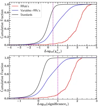
To test the effectiveness of these metrics and deter-mine the threshold values to separate variables from constant stars, we assembled a labeled training set of previously classified objects in SDSS stripe 82 region (hereafter, “S82”). S82 is a ∼ 300 deg2 area spanning 300◦.α.60◦and|δ|.1.25◦that was observed 70-90 times by SDSS in ugriz over a period of 10 years. Nu-merous authors used the resultant well-sampled multi-band light curves to identify thousands of variable stars in the region with high confidence (Ivezi´c et al. 2007;
Sesar et al. 2010;S¨uveges et al. 2012). These labeled ob-jects are extremely useful for studies of variables from both hemispheres thanks to their equatorial location. Although the magnitude range of DES is deeper than that of SDSS, there is sufficient overlap to create a well-populated training set for our study. Using the calibra-tion and variable catalogs from Ivezi´c et al.(2007), we cross-matched 641,710 “standard” (i.e., constant) stars and 16,752 variables in common between SDSS and DES objects. We also identified 296 RRL in common be-tween DES and eitherSesar et al.(2010) orS¨uveges et al. (2012), consisting of 238 and 58 objects of subtype RRab and RRc, respectively.
As an example, we show the cumulative distributions of χ2
ν,b values and “significance” values for the
cross-7 While other metrics such as the Welch-Stetson I Welch & Stetson (1993) and Stetson J (Stetson 1996) indices are widely used and very effective at detecting variability, due to the sparsity of our observations, we chose to use metrics that were agnostic of observation time.
−4 −3 −2 −1 0 1 2 3 4 5 Log10(χ2ν,r) 0.0 0.2 0.4 0.6 0.8 1.0 C um ul at iv e F ra ct io n RRab’s Variables+RRc’s Standards −1 0 1 2 3 Log10(significancer) 0.0 0.2 0.4 0.6 0.8 1.0 C um ul at iv e F ra ct io n
Figure 3. Initial variability metric values for previously
identified objects in S82. Top: Cumulative distribution of log10(χ
2
ν,r). The magenta dashed line denotes the
cho-sen threshold value of 0.5; objects with larger values in any band are considered variable. Bottom: Histogram of log10(significancer). The vertical magenta dashed line
de-notes the chosen threshold value of 1.0; objects with larger values in any band are considered variable. Note that al-though some real RRab are excluded by this cut, most of the non-RRab variables are also excluded.
matched objects in the r band in Figure 3. For both metrics, the threshold values were chosen to minimize the number of non-variable stars that would be sub-ject to subsequent analysis. Any obsub-jects that showed log10(χ2
ν,b) ≥ 0.5 and significance ≥ 1 in any one of
grizY8 were kept for subsequent analysis. When these cuts were applied across all five filter bands, 234 (∼98%) RRab, 57 (∼ 98%) RRc, 5196 (∼ 31%) variable, and 3004 (. 0.05%) standard light curves from S82 met these criteria. These results for our training set are sum-marized in Table 2. Over the entire survey region, ap-proximately∼7×10⁵light curves passed these variabil-ity cuts. We caution that passing this criterion is simply an initial cut and does not imply that these sources are truly variable.
Despite these cuts, a small but non-negligible fraction of the objects identified as “standard” by Ivezi´c et al.
8Unlike the initial cuts we applied to the coadded catalog, we
included theYband in these variability cuts because theY band values were weighted by the photometric uncertainties.
Table 2. Training set of cross-matched S82
objects
SDSS Label Present in DES Passed Cuts
RRab 238 234
RRc 58 57
Variables 16,752 5196
Standards 641,710 3004
Note—Objects were originally identified in
Ivezi´c et al.(2007);Sesar et al.(2010);S¨uveges et al.(2012).
(2007) were still selected. It is possible that some of these objects are truly variable sources that did not dis-play significant changes in the previous studies. Another possibility is erroneous photometry that, while rare, oc-curs sometimes in the Y3Q2 dataset due to incorrectly attributing observations from separate sources to one object or imperfect masking of observations obtained in very poor weather conditions. While these objects may have passed the initial variability cuts, their light curves fit the RRL template poorly, and most of them were re-jected later in our analysis.
All of the selected light curves were corrected for extinction using reddening values from the maps of
Schlegel, Finkbeiner & Davis (1998) multiplied by fil-ter coefficients derived from theFitzpatrick (1999) red-dening law (for RV = 3.1) and the adjustments to the Schlegel, Finkbeiner & Davis(1998) map presented by
Schlafly & Finkbeiner(2011) (see §4.2 in DES Collab-oration (2018) for more details). We then used the extinction-corrected light curves as the input for our template fitting algorithm.
4. CANDIDATE IDENTIFICATION 4.1. RR Lyrae Template
Our current work introduces a novel method of iden-tifying RRab by fitting an empirically derived periodic model to the sparsely sampled multiband light curves. The model has the form:
mb(t) =µ+Mb(ω) +aγb(ωt+φ) (4)
where mb is the measured magnitude in a given band
b at a given time t, µ is the distance modulus, Mb is
the average absolute magnitude in that band,ω= 1/P
is the frequency of the variability (inverse of the period
P), a is the g-band amplitude (the amplitudes of the curves for the other bands are proportional to a), γb
is a periodic shape function, andφ is the phase. Only the four parameters µ, a, ω, φ are estimated during
−0.35 −0.30 −0.25 −0.20 −0.15 −0.10 −0.05 Log10(P) 0.3 0.4 0.5 0.6 0.7 0.8 M b ( P ) g r i z Y
Figure 4. P−Lrelations used in our template fitting
pro-cedure. RRL have nearly constant absolute magnitudes ing
regardless of period. See§4.1for more details.
the fitting process while the forms ofγb andMb(ω) are
fixed. These were derived using well-sampled RRab light curves from S82 (Sesar et al. 2010) and shifted to adjust for slight differences between SDSS and DES filters. A more detailed description of the template construction is included in AppendixA.
Using the same reasoning as Sesar et al. (2017), we chose to exclude RRc from our study because: a) their sinusoidal light curves are difficult to distinguish from light curves from other variable objects such as eclips-ing binaries, b) their small amplitudes would make them difficult to identify in our sparse data, and c) searching over a larger period range to recover their short peri-ods (∼0.3d) would introduce additional common period aliases into our sample. While excluding RRc weakens our sample size for tracing substructure, it is not pro-hibitive since RRc are usually less numerous than RRab. Furthermore, this approach allowed us to use only one generalized RRab shape for our template instead of an ensemble of shapes as inSesar et al.(2017). While they were able to recover a more diverse group of RRL by fit-ting multiple shapes, our approach makes our algorithm more computationally efficient.
The P-L-Z relations were implemented in our tem-plate fitting procedure as P-Lrelations evaluated at a starting metallicity of [Fe/H] = −2.85. However, the values of these offsets between template filter curves were later adjusted to fit the S82 RRL light curves, so this metallicity should not be treated as the true value of the template. Hence, the metallicity value of our tem-plate is somewhat ambiguous. We discuss the effects of the metallicity further in §5.4. The final template P-L relations are shown in Figure 4. More details on how these parameters were derived are presented in Ap-pendixB.
4.2. Template Fitting
In this section, we include a high-level overview of the template fitting procedure. A more detailed description of this process can be found in AppendixC.
To fit the template to a light curve, the algorithm per-forms a grid search over a specified range of frequencies. To prevent misestimated and aliased periods outside of the true range of periods known for RRab, we restricted this range to values corresponding to periods of 0.44 days to 0.89 days following the period-amplitude rela-tion shown in Figure 16 of Sesar et al.(2010). At each frequency gridpoint, the algorithm first calculatesMb(ω)
(see Equation4 and Figure 4) and subtracts these val-ues from the light curve magnitudes in the appropriate band. Then, with the frequency fixed, the model alter-nates between estimating the best-fittingφ using New-ton’s method, and (a, µ) using weighted least squares. The (φ, a, µ) values which minimize the weighted Resid-ual Sum of Squares (RSS) at each frequency gridpoint are chosen as the best-fitting parameters, and act as the starting point for the parameter search at the next gridpoint. The (ω, φ, a, µ) at the global minimum RSS value over the entire frequency grid are chosen as the best-fitting parameters9.
A major strength of this algorithm is that the tem-plate shape is fit simultaneously to the light curve data in all five bands combined. Since there are only four free parameters that must be fit for the entire light curve, unique solutions can be found for sparse light curves with very few measurements in any single band. An ex-ample RSS curve for an RRab from the labeled training set is shown in Figure 5. Because the local minima in the RSS curve are sometimes very close in value, we in-clude the best-fitting values for the top three minima of RSS in our data products for completeness, but do not discuss the results of the 2nd and 3rd minima further in this work.
Our algorithm is also effective at estimating distances. At the best fit parameter estimates, the template fitting algorithm correctly estimated∼81% of the S82 RRL dis-tances to within 3% of the values obtained by Sesar et al.(2010) andS¨uveges et al.(2012) (if available) with an overall standard deviation of 2.8% (see §5.4 for an ex-tended discussion of the uncertainties in distance mod-ulus). The accuracy of the template estimates of both 9 In his study of Cepheid variables,Stetson(1996) also
devel-oped a template fitting method based on least squares. However, instead of using a string-length minimization technique in a single band, we use all the bands simultaneously and used a fixed shape instead of a family of derived template curves calculated for each trial period.
0.5 0.6 0.7 0.8 Period (days) 0 100 200 300 400 RSS
Figure 5. Residual Sum of Squares (RSS) curve for an
RRab originally discovered bySesar et al. (2010). The red arrow denotes the global minimum of the RSS which corre-sponds to the true period of 0.5336 days.
0 250 500 750 1000 MJD - 56250.08 17.5 18.0 18.5 19.0 M ag ni tu de g r i z Y 0.0 0.5 1.0 1.5 2.0 Phase 17.5 18.0 18.5 19.0 M ag ni tu de
Figure 6.Top: Poorly sampled DES light curve of an RRab
originally discovered bySesar et al.(2010) (same star as Fig-ure5). Bottom: Phased light curve of the same source with the period correctly estimated by our algorithm. Note: Pho-tometric uncertainties are smaller than the plotting symbols.
the period and the distance for the training set of RRab light curves is summarized in Table3).
Our algorithm is computationally efficient and only takes ∼3−5 minutes per light curve on an Intel Xeon E5420 processor. The template fitting code returned the estimated parameters of the top three best-fitting templates as well as the features used in the random forest classification detailed in §4.4 and Table 4. The computation time for fitting the template and calculat-ing features for∼7×10⁵ light curves was∼44K CPU
Table 3. Period and distance estimation
accu-racy
Parameter % of RRab within σparameter
1% 3%
∆P /Pprev 88.89 89.74 6.81%
∆D/Dprev 44.64 81.11 2.83%
Note—Pprev and Dprev are the values reported in Sesar et al.(2010) andS¨uveges et al.(2012).
hours. For comparison to a similar analysis, our algo-rithm is>9×faster than the template fitting methods used bySesar et al.(2017), which required∼30 minutes per star.
There are several other well-documented methods available in the literature for identifying RRL in multi-band data (e.g. VanderPlas & Ivezi´c 2015,Hernitschek et al. 2016 and Sesar et al. 2017), which yield excel-lent results for data sets with an average of 35 or more observations per light curve. We present this algo-rithm as an alternative to these other methods for especially sparse multiband data sets (see §5.3 for a discussion of the observational limitations.) The tem-plate and the associated fitting code are available at
https://github.com/longjp/rr-templatesand further de-scribed in AppendixD.
4.3. Feature Selection
While it is possible to identify RRL by visually in-specting their phase-folded light curves, the sheer vol-ume of light curves in our data set makes this classi-fication method unfeasible. Instead, we computed nu-merical features to describe the behavior of the light curves. To assess the specific parameter space occupied by RRab, we compiled a training set consisting of all the cross-matched labeled objects from S82 which passed the initial variability cuts (discussed in§3.2). This left us with a training set of 234 RRab, 57 RRc, 5196 other variable objects, and 3004 “standard” sources. Since we only aimed to identify RRab, we chose a simple identi-fication scheme with two classes: RRab and non-RRab. This resulted in an RRab class with 234 objects and a non-RRab class with 8257 objects.
With the goal of identifying RRab, we chose features which were motivated by how well the light curves fit the RRab template and other observed properties of RRab. As demonstrated in Figure3, RRab have relatively large log10(χ2ν,b) compared to most of the other objects in our
sample. So, to quantify the base variability of the light curve while ignoring spurious signals or missing obser-vations in any particular band, we included the median
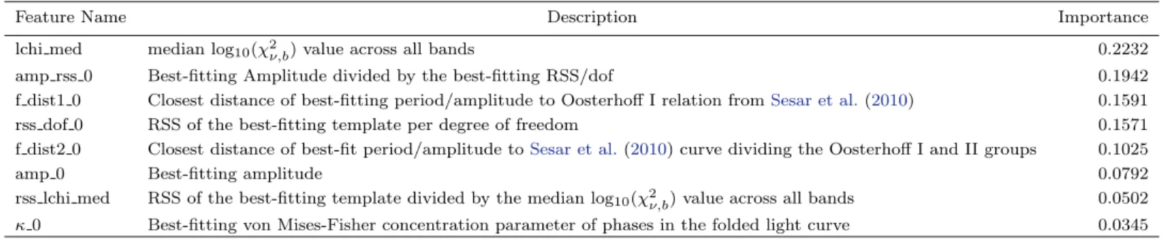
Table 4. Random Forest Features
Feature Name Description Importance
lchi med median log10(χ2ν,b) value across all bands 0.2232
amp rss 0 Best-fitting Amplitude divided by the best-fitting RSS/dof 0.1942
f dist1 0 Closest distance of best-fitting period/amplitude to Oosterhoff I relation fromSesar et al.(2010) 0.1591
rss dof 0 RSS of the best-fitting template per degree of freedom 0.1571
f dist2 0 Closest distance of best-fit period/amplitude toSesar et al.(2010) curve dividing the Oosterhoff I and II groups 0.1025
amp 0 Best-fitting amplitude 0.0792
rss lchi med RSS of the best-fitting template divided by the median log10(χ2ν,b) value across all bands 0.0502
κ0 Best-fitting von Mises-Fisher concentration parameter of phases in the folded light curve 0.0345 Note—All of these feature values for each candidate are included in the electronic version of Table6.
of this value calculated across all five filters as a feature. Additionally, most true RRab should fit the template with small residuals, so we quantified the quality of the best template fits using the RSS per degree of freedom, RSSdof = RSS/(Nobs−4). Then, to amplify the
sepa-ration provided by these two characteristics, we divided the RSSdof by the median log10(χ2ν,b) to form another
feature.
To take advantage of the distinctive amplitude ranges of RRab, we also selected the amplitude of the best-fitting template as a feature. We then created a new fea-ture by dividing this amplitude by the RSSdof, expect-ing that the large amplitudes and excellent template fits of RRab would clearly distinguish them from other ob-jects. We can take advantage of these amplitudes again by evaluating how closely each object matches the ob-servational trends shown by RRab in the first two Oost-erhoff groups (see the introduction for a brief descrip-tion). To measure how closely the objects’ estimated template parameters matched these trends for RRab, we calculated the distance of the object in period-amplitude space from the Oosterhoff I relation measured in Sesar et al.(2010) and their shifted curve which separates the Oosterhoff I and II populations (see their Figure 16 and our Figure12.)
Our last feature attempted to quantify the phase distribution of the observations in each light curve. Period-finding algorithms often recover periods at com-mon aliases, sometimes resulting in light curves with many of their observations clustered near a particular phase. Because light curve phases are periodic, the two-dimensional case of the von Mises-Fisher distribution (Fisher 1953; Jupp & Mardia 1989) is a good approxi-mation. This distribution can be written as:
f(x) =e
κcos(x−µ) 2πI0(κ)
(5)
whereκis the concentration parameter, µis the mean, and I0(κ) is the modified Bessel function of the first kind at order 0. The von-Mises Fisher distribution is akin to a Gaussian distribution wrapped around a cir-cle, where the κparameter is analogous to the inverse of the variance (see§2.2 inSra 2016for a more detailed description). We calculated this concentration param-eter κ for each light curve folded over the best-fitting template period. Light curves with observations highly clustered in phase will have very large values ofκ, aiding in the rejection of objects with aliased periods.
Although our choice of classifier is generally robust against non-informative features, we limited our features to these to make the classifier results easier to interpret. The features are summarized and ranked by their im-portance, or how much they contributed to splitting the data across all the decision trees in our classifier10, in
Table4. These features are shown in Figure7. The de-velopment of additional features to further separate the classes will be explored in future work.
4.4. Random Forest Classifier
To identify likely RRab automatedly and consistently, we trained a random forest classifier (Amit and Geman 1997; Breiman 2001) using these features. The ran-dom forest is a machine learning algorithm that predicts classes for data by combining results from a “forest” of decision trees. Each decision tree consists of a series of nodes where the data is split into subgroups based on the values of a random subset of their features, or characteristics. Before the random forest can make ac-curate predictions, it must be trained to recognize the trends in features that correspond to different classes. Thus, one needs a labeled training set to build the ran-dom forest. Each decision tree uses the labels to build 10 See§1.11.2.5 in thescikit-learndocumentation for more
Figure 7. Features used to identify RRab plotted for the training set. Red points denote previously identified RRab while black X’s are non-RRab. While the RRab clearly oc-cupy a specific region in this feature space, they are not linearly separable.
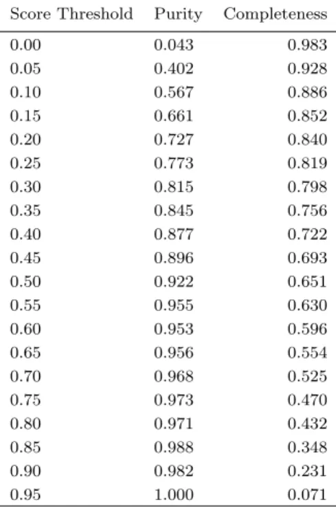
Table 5. Estimated RRab selection
purity & completeness
Score Threshold Purity Completeness
0.00 0.043 0.983 0.05 0.402 0.928 0.10 0.567 0.886 0.15 0.661 0.852 0.20 0.727 0.840 0.25 0.773 0.819 0.30 0.815 0.798 0.35 0.845 0.756 0.40 0.877 0.722 0.45 0.896 0.693 0.50 0.922 0.651 0.55 0.955 0.630 0.60 0.953 0.596 0.65 0.956 0.554 0.70 0.968 0.525 0.75 0.973 0.470 0.80 0.971 0.432 0.85 0.988 0.348 0.90 0.982 0.231 0.95 1.000 0.071
Note—The full version of this table is avail-able in the online data products.
a series of boundaries in feature space that divide the data into their correct classes. Once trained, the ran-dom forest algorithm assigns a score to unlabeled data based on the proportion of trees that identify them as a particular class. Random forest classifiers have been extremely successful in variable star classification (see
Richards et al. 2011 for a comparison with other ma-chine learning techniques), even in the case of sparsely sampled Pan-STARRS PS1 light curves (Hernitschek et al. 2016). Thus, the random forest was a natural choice of classifier for this study.
We created the classifier using the RandomForest
package available in scikit-learn (Pedegrosa et al. 2011). To prevent overfitting to our small training set and ensure repeatability, the classifier contained 500 trees with a maximum depth of 5, and used a random seed of 10.
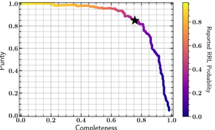
We assessed the performance of our classifier by esti-mating the purity (the percentage of objects classified as RRab that were truly so) and the completeness (the percentage of real RRab that were identified as such) as a function of the class score reported by the random forest. The purity and completeness were estimated us-ing a five-fold cross validation technique, where the data were divided into five test groups and classified based on
0.0 0.2 0.4 0.6 0.8 1.0 Completeness 0.0 0.2 0.4 0.6 0.8 1.0 P ur it y 0.0 0.2 0.4 0.6 0.8 R ep or te d R R L P ro ba bil ity
Figure 8. Purity/Completeness curve for the random forest
classifier trained on cross-matched objects in S82. The black star denotes a classifier-reported score of 0.35, where the purity is ∼85% and the completeness is∼76%. The area under the curve is 0.864.
a classifier trained on the other four groups. The clas-sifier correctly identified 190 of the 234 RRab used to train the random forest as such with a score threshold of
≥35%. As shown in Figure8, defining RRab as objects with a score ≥35% yields a purity of 85% and a com-pleteness of 76%. A common metric used to assess the performance of a classifier is the area under the curve (AUC) shown in Figure 8, which we find to be 0.864. The purity and completeness calculated at other score thresholds are listed in Table 5. We include all other objects with lower scores in our catalog so that other score thresholds can be specified by interested readers. Although an incorrect period estimate led to a worse RSS value for the fit, some RRab with incorrect period estimates were still correctly identified as such by the classifier.
Since our training set was mostly composed of nearby RRab confined to a small region in the survey footprint, it is imperative to assess our classifier performance using other samples of RRL. To this end, we cross-matched our sample with external surveys in §5.2 and applied our method to simulated RRab light curves at fainter magnitudes in§5.3.
5. CATALOG DESCRIPTION 5.1. Visual Validation
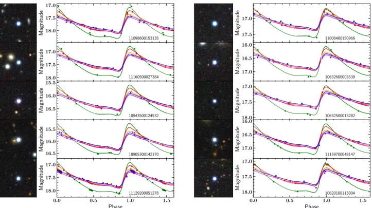
We applied the classifier to the∼7×10⁵objects with template fits and found 8026 RRL candidates with a score≥0.35. Although most of our candidates were in-deed RRL found in other surveys, there were still some non-stellar interlopers in the sample due to the lenient initial cuts on the shape of the photometric point-spread function (§2.2). Thus, we visually inspected all RRab candidate light curves and their DR1 coadded images.
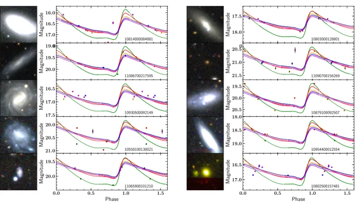
After visually validating the candidates and removing any objects with non-RRL classifications in the Simbad database (Wenger et al. 2000), 1786 objects were dis-carded and 5783 RRL candidates remained in the cat-alog, with the rest too ambiguous to confirm. A sam-ple of visually verified candidates with high (p > 0.94) and low (p < 0.36) classifier scores are shown in Fig-ures9 and 10, respectively. The most typical contami-nants in the sample were extended sources. Given our lenient selection criteria described in§2.2, it is not sur-prising that some of these objects made it into our final sample. Examples of candidates that were re-jected by visual inspection as being extended sources are shown in Figure11. The full catalog of candidates, their best-fit parameters, and their features are available athttps://des.ncsa.illinois.edu/releases/other/y3-rrl. A sample view of this catalog is shown in Table 6. Ap-pendix E contains a detailed description of these data products.
Although the light curves have been visually in-spected, further photometric observations of some ex-tremely poorly sampled candidate light curves would be useful to confirm their classification. One may wish to remove these more uncertain candidates from their anal-ysis by only considering objects with a larger minimum number of observations. Some of these candidates have gaps in observations near their maximum and mini-mum brightness, providing poor constraints on their estimated amplitudes and mean magnitudes. There-fore, we assigned a flag to each object based on how its phase-folded light curve is sampled. An object with fewer than two observations near its minimum bright-ness (0.55≤phase<0.87, which we chose to encompass both the near-constant portion of the light curve where other authors chose their minimum phase (e.g.,Vivas et al. 2017) and the 10% quantile of template magnitudes) will receive a “flag minmax” value of 1, while an ob-ject with<2 observations near its maximum brightness (0.96 ≤phase <1 or 0 ≤ phase<0.05 corresponding to the 90% quantile in template magnitudes) receives a “flag minmax” value of 2. Objects missing observations near both of these receive a flag value of 3.
Figure12shows a Bailey (period-amplitude) diagram of the candidates rejected by the classifier or our visual checks plotted in black, visually accepted candidates shown in red, and ambiguous candidates in blue. We plot the Oosterhoff I (Oosterhoff 1939) relation and the curve dividing groups I and II from (Sesar et al. 2010) which we used in the calculation of our features in solid and dashed black lines. Many of these ambiguous can-didates are likely RRab, but cannot be classified as such with high confidence in this work. Due to the sparse
Phase 17.0 17.5 18.0 Magnitude 11098600153135 17.0 17.5 18.0 Magnitude 11160500027384 15.5 16.0 16.5 Magnitude 10943500124532 15.5 16.0 16.5 Magnitude 10905300142170 0.0 0.5 1.0 1.5 Phase 17.0 17.5 18.0 Magnitude 11129200051278 Phase 17.0 17.5 Magnitude 11006400150966 16.0 16.5 17.0 Magnitude 10632600003539 17.0 17.5 18.0 Magnitude 10632500013282 16.0 16.5 17.0 Magnitude 11159700048147 0.0 0.5 1.0 1.5 Phase 17.0 17.5 18.0 Magnitude 10620100113004
Figure 9. Sample of DES coadded images and representative light curves of visually accepted RRL candidates with classifier
scores exceeding 0.94, labeled with their Y3Q2 ID number. The observations and templates are colored by filter using the same convention as Figure6. 0.0 0.5 1.0 1.5 20.0 20.5 Magnitude 10992600031952 19.0 19.5 20.0 Magnitude 10854400008649 18.5 19.0 Magnitude 11057500021052 21.0 21.5 22.0 Magnitude 10955000103148 0.0 0.5 1.0 1.5 Phase 21.5 22.0 Magnitude 10594600004013 0.0 0.5 1.0 1.5 20.5 21.0 Magnitude 11146900058729 19.0 19.5 20.0 Magnitude 10864400140579 19.0 19.5 Magnitude 11161900945716 20.5 21.0 21.5 Magnitude 10890200083304 0.0 0.5 1.0 1.5 Phase 18.5 19.0 Magnitude 11041500084646
Figure 10. Sample of DES coadded images and representative light curves of visually accepted RRL candidates with classifier
scores below 0.36, labeled with their Y3Q2 ID number. The observations and templates are colored by filter using the same convention as Figure6.
0.0 0.5 1.0 1.5 16.0 16.5 17.0 Magnitude 10814000084881 19.0 19.5 20.0 Magnitude 11086700217595 16.5 17.0 17.5 Magnitude 10930500092149 20.0 20.5 21.0 Magnitude 10558100130021 0.0 0.5 1.0 1.5 Phase 19.5 20.0 Magnitude 11065900101210 0.0 0.5 1.0 1.5 17.5 18.0 Magnitude 10803000128801 20.5 21.0 21.5 Magnitude 11090700156269 19.5 20.0 20.5 Magnitude 10879100092507 18.0 18.5 19.0 Magnitude 10954400012554 0.0 0.5 1.0 1.5 Phase 16.5 17.0 Magnitude 10802500157481
Figure 11. Sample of DES coadded images and representative light curves of visually-rejected candidates (extended sources
or possible supernova) that passed the classifier score threshold, labeled with their Y3Q2 ID number. The observations and templates are colored by filter using the same convention as Figure6.
Table 6. DES RRab Candidates
DES Y3Q2 ID α δ hgi hri hii hzi hYi P Ag µ p
[deg, J2000] [mag] [d] [mag]
11136400113264 0.000107 -59.559187 17.657 17.500 17.547 17.535 17.588 0.6415 0.551 16.90 0.436 10646400013129 0.013042 -2.430057 17.234 17.052 17.099 17.103 17.252 0.4938 1.151 16.66 0.733 11004800140792 0.131498 -41.482218 19.229 19.096 19.125 19.195 19.145 0.5893 1.137 18.69 0.568 11108800089990 0.134204 -54.295118 15.754 15.625 15.557 15.554 15.571 0.6698 0.469 14.97 0.659 10595200009863 0.283437 1.178535 17.986 17.922 17.908 17.868 17.869 0.5480 1.033 16.96 0.886 Note—DES Y3Q2 ID: DES Y3Q2 quick object id number. α: Right Ascension. δ: Declination. hgrizYi: Mean
extinction-corrected magnitude. P: Best-fit period. Ag: Best-fit amplitude in DESg. µ: Best-fit distance modulus.
p: RRab score assigned by the classifier. The full version of this catalog, including feature values and cross matching information, is available in the online data products athttps://des.ncsa.illinois.edu/releases/other/y3-rrl.
nature of our observations, we cannot detect amplitude modulations such as those arising from the Blaˇzko ef-fect (Blaˇzko 1907), although we did recover five out of twelve Blaˇzko RRL previously identified in the Catalina Surveys (Drake et al. 2014,2017).
Figure 12. Bailey diagram of template-estimated
ampli-tudes and periods for objects that passed the initial variabil-ity cuts in black and visually accepted RRab identified by our classifier in red. Ambiguous candidates that could not be visually accepted are plotted in blue. We overplot the Oosterhoff I relation and the curve dividing the Oosterhoff I and II populations fromSesar et al. (2010) in black solid and dashed lines, respectively. The abundance of objects with periods ofP = 0.5 day denotes a common alias of the 1 day rotation period of the Earth.
5.2. Comparison with Overlapping Catalogs The DES footprint has significant overlap with other surveys, such asGaia (Gaia Collaboration et al. 2016), Pan-STARRS (Chambers et al. 2016), the Catalina Sur-veys (Drake et al. 2009), and the Asteroid Terrestrial-impact Last Alert System (ATLAS: Tonry et al. 2018). We used our cross-matches with these external RRab catalogs to independently assess the performance of our algorithm at the different magnitude ranges probed by these surveys. We used the SkyCoord package in
astropy(Astropy Collaboration 2018) to select matches within 100of DES objects while removing duplicates. De-tails for each individual survey are presented in the fol-lowing paragraphs and summarized in Table 7, while Figure13shows the respective overlaps with DES.
Clementini et al.(2018) found over 1.4×10⁵ RRL in GaiaDR2, including∼5×10⁴that were previously un-known. These variables were identified from multiband (G, GBP, GRP) light curves that had at least 12
obser-vations in G (see Figure 10 inHoll et al. 2018). While the Gaia temporal coverage is very uneven, their RRL catalog spans the entire sky (see Figure 26 inClementini et al. 2018) and has high purity (∼91%), making it an excellent independent check of our method at brighter magnitudes. 4609 of theGaiaDR2 RRabs were present
in our initial stellar catalog (§2.2) and 3227 (∼70%) were identified as such. To assess this recovery another way, if we create a purity vs. completeness curve from these cross-matches like the one shown in Figure 8, we find an AUC of 0.727. As we have significantly fewer single-band observations thanGaia DR2, it is not surprising that we do not recover all of their RRab.
We also searched for RRab discovered in Pan-STARRS PS1 by Sesar et al. (2017). Like DES, Pan-STARRS has sparsely-sampled multiband light curves andSesar et al.(2017) employed a similar template fit-ting method to identify these variables. However,Sesar et al.(2017) used the final data release of PS1 with an average of 67 observations per object (compared to our median of 18). We adopted their suggestedab score cut of 0.8 to select only RRab. As Pan-STARRS primarily surveyed the Northern hemisphere, we found just 1021 RRab in our initial stellar catalog, but we identified 805 (∼79%) as such, with an AUC of 0.681. As the Pan-STARRS light curves are the most similar to the DES Y3 ones out of all the external catalogs under consid-eration, our similar classification results show that our approach is similarly effective as the methods used by
Sesar et al.(2017).
The Catalina Surveys RRL catalog (Drake et al. 2013a,b,2014;Torrealba et al. 2015; Drake et al. 2017) is based on a wide-field (26,000 deg2) time series sur-vey that probes the variable sky to a depth of V ∼
19−20 mag. The observations are unfiltered and col-lected in sequences of four images equally spaced over 30 minutes in each pointing (Drake et al. 2009). After sev-eral years of operation, the Catalina Surveys have over 200 observations for most of their variables (Drake et al. 2014), which makes the catalog largely complete. Given the limited magnitude overlap between the Catalina Surveys and DES, we only found 1463 of their 32775 RRab in our initial stellar catalog, but we identified 1185 (∼81%) as such, with an AUC of 0.733.
ATLAS, a planetary defense initiative with a high cadence well suited for variability studies, recently re-leased its first catalog of variable stars (Heinze et al. 2018). Thus far, ATLAS has at least 200 observations across two filters (c, o) over one-fourth of the sky. We select RRab stars from the ATLAS DR1 variable star catalog using the suggested CasJobs query in Appendix 10.2 of Heinze et al. (2018). As ATLAS is based in the Northern hemisphere and quite shallow compared to DES (r≈20 mag), we only have 484 of their 21061 RRab in our initial stellar catalog but identify 391 (∼
81%) as such, with an AUC of 0.635. This recovery rate is quite similar to the ones for Pan-STARRS and the Catalina Surveys.
Table 7. Description of Selected External RRL Catalogs and their Overlap with DES
Survey Area Filters Depth Observational Nobs RRab
[sq deg] cadence total in DES % found
SDSS stripe 82 ∼300 ugriz g≤21 most observed every 2 days 70-90 447 238 75
Gaia DR2 all sky GBP, G, GRP G∼21 uneven, follows Gaia scanning law 12-240 140,000 4609 70 Pan-STARRS PS1 ∼30000 grizY r≤21.5 2 same-band obs. sep. by 25 min ∼67 35,000 1021 79 Catalina Surveys ∼9000 unfiltered V≤19-20 4 obs. within 30 min &200 32,775 1463 81
ATLAS ∼13000 c, o r∼20 4×per night ∼200 21061 484 81
DES single epoch ∼5000 grizY g∼23.5 irregular ∼50∗ 5783 5783 –
Note—The details of DES are listed for comparison. (*): by the end of the survey (Y6)
16 18 20 22 100 101 102 103 N Gaia DR2 16 18 20 22 100 101 102 103 Pan-STARRS PS1 16 18 20 22 DES< r > 100 101 102 103 N Catalina Surveys DR2 16 18 20 22 DES< r > 100 101 102 103 ATLAS DR1
Figure 13. Histograms of magnitudes of RRab stars from external catalogs cross-matched with our DES initial stellar catalog,
as a function of the extinction-corrected weighted average coadded DESr magnitude. Top left: Gaia DR2. Top right: Pan-STARRS PS1. Bottom left: Catalina Surveys DR2. Bottom right: ATLAS. Blue curves show the RRab from each catalog that were present in our sample before applying any cuts, while red curves show those that were identified as RRab in our analysis. Black curves show the distribution of DES RRab candidates and are the same in all panels. The overdensities atr≈18.8 and
r≈21.2 correspond to the LMC outskirts and the Fornax dSph. Our catalog is deeper than the others by∼1,1,2 and 4.5 mag, respectively.
In addition to searching for RRab candidates with pre-vious identifications from the aforementioned wide-field surveys, we also checked for overlaps near the Magellanic Clouds (Soszy´nski et al. 2016), the Fornax dSph (Bersier & Wood 2002), the Sculptor dSph (Mart´ınez-V´azquez et al. 2016), in the General Catalogue of Variable Stars (Samus’ et al. 2017), and in the SIMBAD database (Wenger et al. 2000). To the best of our knowledge, and based on publicly available catalogs, 1795 (nearly 31% of our sample) are newly-discovered RRab candidates. Al-though the external catalogs under consideration are not
complete, the fraction of their RRab recovered by our analysis is consistent with our estimate of∼75% com-pleteness. Our method is just as effective (if not more so) at recovering RRL from sub-optimally sampled data than the methods used in comparable surveys.
Although we recover most of the RRab in the afore-mentioned overlapping catalogs, we can see from the AUC of each of these that there is a marked degra-dation in our algorithm’s performance when applied to light curves outside our S82 training set. Thus, we use their AUC values to construct a confidence interval for
the performance of our classifier. With the AUC of the training set and all four of these external cross-matches, we find a mean AUC of 0.728 with a standard deviation of 0.077. From this, we can determine that our classifi-cation methods have a lower effiency for fainter RRab. Unfortunately, we do not have well-characterized train-ing data in a comparable filter system for fainter RRab, so we tested this with simulated light curves.
5.3. Estimated Recovery Rates and Uncertainties from Simulated Data
To estimate the robustness of our results for the noisier photometry at fainter magnitudes, we followed a method similar toMedina et al.(2018) and applied our method to simulated light curves with known light curve param-eters in the DES filter system. We created the simu-lated light curves by sampling the smoothed templates of Sesar et al. (2010) in gatspy (VanderPlas & Ivezi´c 2015) with the DES cadence from different areas of the survey. We shifted these light curves to various distances by adding the appropriate distance modulus and insert-ing scatter in the observations based on the magnitude-dependent uncertainty relations we found in§3.1(shown in Figure2). AppendixFcontains further details on the construction of these simulated light curves.
Figure14shows the recovery rates of both the classi-fier and the period as a function of magnitude and total number of observations. As expected, the recovery rate of our algorithm decreases significantly with increasing distance modulus. This is mostly due to the larger pho-tometric uncertainties and fewer observations due to the brighter limiting magnitudes for the redder bands (see
§2.1). We see that the accuracy of the period estima-tion decreases following the trend of increasing photo-metric errors shown in Figure14, and dramatically im-proves with increasing total number of observations up to N ∼20. As expected, the RRab classification accu-racy follows a similar trend. We find that our template fitting recovers the true period to within 1% for 95% of the simulated light curves with N=20 observations.
Beyond assessing our classifier performance with these simulated light curves, we can also use them to esti-mate the uncertainties of the best fitting template pa-rameters. To make sure we treat light curves with especially poor phase coverage separately, we divided the simulated light curves into groups based on their “flag minmax” values (described in§5.1). Then, we sub-divided those into bins of two observations and 0.5 mag-nitude wide in N and µ, respectively. In each of these bins, we calculate the fraction of light curves with pe-riod estimates within 1% of their input values for each phase sampling group. To quantify the uncertainty of
Table 8. Coefficients for Parameter Uncertainties
Value p0 p1 p2 p3
σ(∆P /P) 4.8585×10⁻¹ -4.5912×10⁻² 1.5636×10⁻³ -1.7574×10⁻⁵
σ(∆a) 1.5333 -1.5101×10⁻¹ 5.3006×10⁻³ -6.1034×10⁻⁵ Note—The best fit 3rd degree polynomial is of the form σ(Value) =p0+
p1N+p2N2+p3N3.
the period estimates, we calculated the standard devi-ation of ∆P/P = Pest−Ptrue/Ptrue, where the “est”
subscript represents the parameter estimate from the template fitting and “true” represents the input value of the simulated light curve. Likewise, we calculated ∆a=aest−atrueto quantify the uncertainty of the
am-plitude estimates. The number of light curves included in each bin differs widely, so we estimate the spread of these uncertainty values within each subgroup with jackknife resampling. These results are shown in Figure
14.
Other than fluctuations due to the small sample sizes in some of the bins, these values follow expected trends. When there are fewer observations to constrain the pa-rameter values during the template fitting, both the pe-riod and the amplitude are more uncertain, with these values beginning to stabilize around N=20 observations. In distance space, the parameter estimates are generally low until µ≈20, where the brighter detection limits of the redder filters decrease the number of observations in the light curves. We have very few simulated light curves that are missing observations near their maxi-mum only or both their maximaxi-mum and minimaxi-mum (the blue and orange points in Figure14), so we cannot draw any definitive conclusions about the effect of phase sam-pling on the estimation of these parameters. We assign these parameter uncertainties to the real RRab candi-dates based on the best fitting 3rd degree polynomial to the trends in N observations for all simulated light curves. We do not assign uncertainties to objects with
N >43 observations due to a lack of simulated data with
that sampling. We also do not report these uncertainties for objects not identified as RRab by the classifier since these simulated light curves do not accurately represent the behavior of non-RRab. The coefficients of the best fitting polynomials are included in Table8 and the un-certainties are included in the full catalog described in AppendixE.
The uncertainty of the remaining parameter φis sig-nificantly more difficult to constrain. Phases for individ-ual observations in the folded light curves are calculated using phase = (MJD/P) mod 1. Any small offset in
5 10 15 20 25 30 35 40 0.0 0.2 0.4 0.6 0.8 1.0 F ra ct io n R ec ov er ed by C la ss ifi er Well sampled Missing obs near min Missing obs near max Missing obs near both
15 16 17 18 19 20 21 22 0.0 0.2 0.4 0.6 0.8 1.0 F ra ct io n R ec ov er ed by C la ss ifi er 5 10 15 20 25 30 35 40 0.0 0.2 0.4 0.6 0.8 1.0 F ra ct io n w it hi n 1% in P 15 16 17 18 19 20 21 22 0.0 0.2 0.4 0.6 0.8 1.0 5 10 15 20 25 30 35 40 0.0 0.1 0.2 0.3 0.4 σ (∆ P / P ) 15 16 17 18 19 20 21 22 0.0 0.1 0.2 0.3 0.4 5 10 15 20 25 30 35 40 N observations 0.0 0.5 1.0 σ (∆ a ) 15 16 17 18 19 20 21 22 µ 0.0 0.5 1.0
Figure 14. Recovery rates and parameter uncertainties as a function of the number of observations in the light curves and
distance modulusµ. Colored points denote the behavior of the recovery fractions or parameter offsets for light curves with the phase sampling flags described in §5.1. Uncertainties on these values were estimated using jackknife resampling. The black points in the upper right corner of the bottom panels show the representative width of the bins in each column. Dashed grey lines show the best fitting 3rd degree polynomial to the trends shown by the combined simulated data used to assign uncertainties in the RRab catalog. The coefficients for these fits are listed in Table8. First row: Fraction of simulated RRab light curves which received a classifier score ≥0.35. Second row: Fraction of estimated periods within 1% of the true input values. Third row: Standard deviation of the percent difference in period. Bottom row: Standard deviation of the offset in amplitude. Note: