(Article begins on next page)
The Harvard community has made this article openly available.
Please share how this access benefits you. Your story matters.
Citation
Liublinska, Viktoriia. 2013. Sensitivity Analyses in Empirical
Studies Plagued with Missing Data. Doctoral dissertation, Harvard
University.
Accessed
April 17, 2018 4:06:29 PM EDTCitable Link
http://nrs.harvard.edu/urn-3:HUL.InstRepos:11124841
Terms of Use
This article was downloaded from Harvard University's DASH
repository, and is made available under the terms and conditions
applicable to Other Posted Material, as set forth at
http://nrs.harvard.edu/urn-3:HUL.InstRepos:dash.current.terms-of-use#LAA
A dissertation presented by
Viktoriia Liublinska to
The Department of Statistics in partial fulfillment of the requirements
for the degree of Doctor of Philosophy in the subject of Statistics Harvard University Cambridge, Massachusetts April 2013
Sensitivity Analyses in Empirical Studies Plagued with
Missing Data
Abstract
Analyses of data with missing values often require assumptions about missingness mechanisms that cannot be assessed empirically, highlighting the need for sensitiv-ity analyses. However, universal recommendations for reporting missing data and conducting sensitivity analyses in empirical studies are scarce. Both steps are often neglected by practitioners due to the lack of clear guidelines for summarizing missing data and systematic explorations of alternative assumptions, as well as the typical attendant complexity of missing not at random (MNAR) models.
We propose graphical displays that help visualize and systematize the results of sensitivity analyses, building upon the idea of “tipping-point” analysis for experi-ments with dichotomous treatment. The resulting “enhanced tipping-point displays” (ETP) are convenient summaries of conclusions drawn from using different modeling assumptions about the missingness mechanisms, applicable to a broad range of out-come distributions. We also describe a systematic way of exploring MNAR models using ETP displays, based on a pattern-mixture factorization of the outcome distri-bution, and present a set of sensitivity parameters that arises naturally from such a factorization. The primary goal of the displays is to make formal sensitivity analyses more comprehensible to practitioners, thereby helping them assess the robustness of experiments’ conclusions. We also present an example of a recent use of ETP displays
The last part of the dissertation demonstrates another method of sensitivity anal-ysis in the same clinical trial. The trial is complicated by missingness in outcomes “due to death”, and we address this issue by employing Rubin Causal Model and principal stratification. We propose an improved method to estimate the joint poste-rior distribution of estimands of interest using a Hamiltonian Monte Carlo algorithm and demonstrate its superiority for this problem to the standard Metropolis-Hastings algorithm.
The proposed methods of sensitivity analyses provide new collections of useful tools for the analysis of data sets plagued with missing values.
Title Page . . . i
Abstract . . . iii
Table of Contents . . . v
Acknowledgments . . . vii
1 Missing Data in Empirical Studies 1 1.1 Missing Data Mechanisms . . . 1
1.2 Parameter Estimation with Incomplete Data . . . 6
1.3 Standards of Missing Data Reporting . . . 11
1.3.1 Important Missing Data Summaries . . . 14
1.3.2 Assessing the Overlap Between Respondents and Nonrespondents 17 2 Sensitivity Analysis for Partially Missing Binary Outcomes in a Clin-ical Trial with Two Arms 22 2.1 Introduction . . . 22
2.2 Sensitivity Analyses for Studies with Missing Data. . . 26
2.3 Enhanced Tipping-Point Displays for Studies with a Binary Outcome 28 2.3.1 Simulated Example with a Binary Outcome . . . 33
2.3.2 Real-data Example . . . 40
2.4 Discussion . . . 61
3 Sensitivity Analysis using Enhanced Tipping-Point Displays for Stud-ies with a Dichotomous Treatment and Partially Missing Outcomes. 63 3.1 Introduction . . . 63
3.2 General Framework for ETP Displays . . . 65
3.2.1 Example with a Continuous Outcome . . . 67
3.3 Exploring MNAR models with ETP displays . . . 74
3.4 Software for ETP Displays . . . 82
3.5 Discussion . . . 83
ies with Missing Data 84
4.1 Introduction . . . 84
4.2 Description of the Clinical Trial . . . 88
4.3 Application of Principal Stratification to the Clinical Trial . . . 89
4.3.1 Notation and Identification of Principal Strata . . . 89
4.3.2 Assumptions and Estimands of Interest . . . 92
4.3.3 Model Specifications for Potential Outcomes and Principal Strata Membership . . . 97
4.4 Application of HMC Method to PS Computations . . . 102
4.4.1 General Overview . . . 102
4.4.2 Example 1: Canvassing and Voter Turnout . . . 104
4.4.3 Example 2: Influenza Vaccination and Flu . . . 106
4.5 Results and Discussion . . . 109
5 Conclusion 112 A Missing Data Handling 114 A.1 Violation of Distinctness Under MAR . . . 114
B ETP Displays 117 B.1 Minimal Sufficiency for EF and NEF . . . 117
B.2 Approximate Degrees of Freedom . . . 120
C HMC Algorithm for PS Framework 122 C.1 Bayesian Updating for PS Framework with HMC Steps . . . 122
C.2 Data and Models for Example 1 . . . 126
C.3 Data and Models for Example 2 . . . 129
I would like to express my sincere appreciation to my principal advisor and men-tor, Professor Donald B. Rubin, for the guidance and advice that he has given me throughout my PhD program. During our extended conversations I learned a lot about the art of balancing rigor and pragmatism in real-world problems, guided by statistical intuition. It enabled me to grow and mature as a statistician.
I also thank Roee Gutman for helpful discussions and for assisting in the imple-mentation of the data imputation procedure, Soteira, Inc. for permission to use their data, and Arman Sabbaghi for the assistance with the implementation of the HMC algorithm. I am very grateful to Dr. Gregory Campbell for pointing us to the origi-nal publication on related tipping-point aorigi-nalyses, and for serving on my dissertation committee and providing insightful comments.
My gratitude goes out to Professor Xiao-Li Meng for his mentorship, endless enthusiasm and continuous supply of innovative ideas and new opportunities for his students. I enjoyed being part of the Happy Team and I took away a lot from this experience. I thank Professor Carl Morris for advising me during the earlier years of my PhD program and helping me refine my research skills, and Professor Joe Blitzstein for being an incredible pedagogy mentor. I thank the entire Department of Statistics for creating an welcoming, but challenging, atmosphere that helped me develop as a researcher and as a teacher.
Lastly, I would like to give thanks to my wonderful fianc´e, Yves Rene Chretien, for supporting and inspiring me on my PhD journey.
Missing Data in Empirical Studies
The best solution to handle missing data is to have none.
- R.A. Fisher
1.1
Missing Data Mechanisms
When Ronald A. Fisher and Jerzy Neyman were laying the foundation of modern Statistics at the beginning of the 20’th century, the problem of missing data naturally emerged from the applied work conducted by researchers in various fields. One of the first published methods to account for missing observations was developed for field experiments inAllan and Wishart(1930). It was later generalized inYates(1933) and is now regarded as a classical method of handling missing data using ANOVA (Little and Rubin 2002, p. 28). M’Kendrick (1925) studied numerous medical data and, when calculating the infection rate in the population, proposed a method to solve the issue with unobserved exposure indicator. His approach was later recognized to be a
values, the EM algorithm (Dempster et al. 1977; Meng 1997). Wilks (1932) was the first to formally employ method of maximum likelihood, introduced by R. A. Fisher a decade earlier, to provide inference on population parameters in a bivariate normal setting with missing observations.
R. A. Fisher, the greatest statistician of his time, was undoubtedly right by imply-ing that the most effort should be devoted to prevention of missimply-ing data. However, it is almost inevitable that the issue will come up in applications, and most data analysis procedures are not designed to handle it. The problem of non-random at-trition and nonresponse1 in survey research as well as missing data in randomized experiments has been widely addressed in the literature (Rubin 1987; Schafer 1997; Little and Rubin 2002; Allison 2001; McKnight 2007). Nevertheless, up until a half a century later, missing values in applied work were handled primarily by editing or case deletion (Schafer and Graham 2002). Only with the formalization of a frame-work of inference from incomplete data developed in Rubin (1976), the research of methods to handle missing data began to gain momentum.
Missing data pose a major problem for experiments as well as observational stud-ies. If proper randomization was performed, the presence of missing data jeopardizes the original balance of the design and may lead to invalid inferences if not handled properly. Observational studies also suffer from missing data in covariates that are believed to be important in predicting the treatment and outcome, or in the out-come itself, especially if the missing data mechanism is unknown, which is usually
1Here and throughout the article we assume item nonresponse, implying that some information
about each missing unit is available.
decreased generalizability of findings, and biased parameter estimates.
Here we adopt a standard approach to define and classify missing data. A value is consideredmissing if it is potentially observable and meaningful for analysis, although not available in the data set at hand. With N units in the dataset, let XXX = (xik) =
(XXX1, XXX2, . . . , XXXK) be theNxK matrix of baseline variables (covariates, orpredictors),
and let YYY = (yij) = (YYY1, YYY2, . . . , YYYJ) be the NxJ matrix of outcome measures (or dependent variables). It is important to distinguish missingness in baseline predictors and in outcomes because it may have to be handled differently (Little 1992; Moons et al. 2006; Newgard and Haukoos 2008).
We define a matrix of missingness indicators for the outcomes, DDDY = (dij), such
that dij = 1 if unit i is missing the jth outcome. Analogously, a matrix of
miss-ingness indicators for the baseline variables is defined as DDDX = (dik), and we let
DDD = (DDDX, DDDY). The paramount idea introduced in Rubin (1976) suggests that we
need to regard the dij as random variables, and offers a straightforward way to define
missing data mechanisms through distributions on thedij.
Let a set YYYobs = {yij | dij = 0} contain the observed values among the
out-comes, and a set YYYmis contain the missing elements of the matrix YYY, such that
YYY = (YYYobs, YYYmis); note thatYYYobs andYYYmis are not matrices, but rather collections of
elements of the matrixYYY, where, formally, the setsobs and misare functions ofDDDY.
Analogous sets can be defined for the matrix of baseline variables,XXX = (XXXobs, XXXmis).
Also, letf(DDD|XXX, YYY;φφφ) be the conditional distribution of missingness indicators given all data values, observed and missing, and unknown vector-parameter φφφ.
for each possible value ofφφφ,
f(DDD |XXX, YYY;φφφ) =f(DDD |φφφ) for allDDD,XXX, andYYY.
In other words, in a simple case with one vector of outcomes and no predictors (K = 1 and J = 0), missing values can be viewed as randomly deleted. However, in higher dimensions, K > 1 or J >0, or both, it is allowed for the missingness indicators to interact, though independently from the data.
It is rarely the case that the MCAR assumption holds in practice. One scenario where the MCAR assumption is plausible is when the data were deliberately not collected, or missing by design (Rubin 1987). The less restrictive missing at random
(MAR) assumption holds if, for each possible value ofφφφ,
f(DDD |XXX, YYY;φφφ) =f(DDD |XXXobs, YYYobs;φφφ) for the observedDDD,XXXobs, andYYYobs,
and for all XXXmis and YYYmis, i.e., if the distribution of missingness indicators depends
only on the observed covariate and outcome values. Although this is how MAR assumption was defined originally in Rubin (1976) for the purpose of Bayesian or direct-likelihood inference, it is sometimes mistakenly employed for sampling distri-bution (or frequentist) inference based on a large-sample theory, e.g., constructing confidence intervals (seeHeitjan and Basu 1996).
A stochastic generalization of MAR that allows to utilize frequentist inference, called a “MAR mechanism” in Little and Rubin(1987), was formally called missing
is true:
f(DDD |XXX, YYY;φφφ) = f(DDD |XXXobs, YYYobs;φφφ) for all DDD,XXX andYYY ,
and for each possible value of φφφ. In other words, the missingness should depend on the observed data only, and it should hold for all realizations of the missing-data pattern DDD and random variables XXX and YYY, not just for the observed ones. This condition requires analysts to consider a hypothetical missingness mechanism even in cases when all values in the data were observed, as long as some of them could potentially have been missing. However, MAR would hold if, for units with covariate or outcome missingness depending on the underlying values, all values were observed in a current realization. In addition, Little (1995) introduced the term covariate-dependent (CD) missingness for situations with no missingness in predictors (XXX =
XXXobs). CD missingness is a special case of MAAR when the missingness mechanism
depends only on predictors and not on the outcomes, i.e.,
f(DDD |XXXobs, YYY;φφφ) = f(DDD |XXXobs;φφφ) for allDDD,XXXobs andYYY,
for each possible value ofφφφ. In fact, this assumption is the one most commonly used in practice, although many studies erroneously report using MAR assumption.
Assume that the joint distribution of outcomes YYY and predictors XXX has a prob-ability model f(YYY , XXX | θθθ), governed by unknown vector-parameter θθθ, and suppose we are interested in estimating θθθ. The missing data are said to be ignorable for the purpose of likelihood-based inference forθθθif MAR is satisfied and parametersφφφcarry
2002). The term “ignorable” comes from the fact that f(DDD | XXXobs, YYYobs;φφφ) may be
“ignored” (or dropped) from the likelihood without altering the likelihood function (or posterior distribution) ofθθθ.
If either the distinctness ofφφφandθθθor MAR is not met, missing data are considered
nonignorable. Violation of distinctness is less consequential than violation of MAR, because the likelihood-based inference will still produce consistent, although generally inefficient, estimates, whereas, violation of MAR is often critical (see Appendix A.1
for an example of nonignorable MAR mechanism). If the missingness mechanism does not satisfy MAR, it is regarded as missing not at random (MNAR). Analysis of data with MNAR missingness requires specifying a full-data likelihood f(YYY , DDD, XXX | θθθ, φφφ), including a model for the missingness mechanismf(DDD |XXX, YYY;φφφ), in order to produce a generally valid likelihood-based inference. In practice, these models require making assumptions about the distribution of missing values that often cannot be assessed empirically, and, therefore, the obtained results should be subjected to sensitivity analyses.
1.2
Parameter Estimation with Incomplete Data
The most basic approach to handle data with missing values is complete-case (listwise deletion) or available-case (pairwise deletion) analysis. However, quite a few research articles were written about the shortcomings of this approach (e.g., Rubin
2I.e., are in disjoint parameter spaces; the concept can be extended to Bayesian inference by
requiring two vector-parameters,θθθ andφφφ, to be a priori independent.
2006; Carpenter and Kenward 2008; Liublinska and Rubin 2012).
Many superior methods were developed during a second half of the 20th century. One class of methods utilizes the idea introduced by Horvitz and Thompson (1952), which suggests weighting responses by inverse-probability of observation to produce unbiased estimate of population averages (?Little and Rubin 2002, section 3.3). One can think of this procedure as a reconstruction of the population of interest, with each weight corresponding to an approximate number of units in the population that the observed response represents.
The Horvitz-Thompson estimator was originally proposed for analysis of surveys with sampling weights set in advance and the estimator is most efficient when the true weights are known. However, in observational studies it is largely impossible to know the missingness mechanism exactly and weighting methods require modeling response probabilities using available covariates. Estimates based on weighting responses by the estimated propensity to respond can be very unstable; they rely heavily on the validity of the proposed propensity model. In addition, if very few respondents are similar to nonrespondents, they would have a disproportionately large effect on the estimate, resulting in large uncertainty bounds. Inference from this class of methods is mainly focused on marginal population characteristics, e.g., average response, al-though it can be extended to consistently estimate parameters from the conditional distribution f(YYY | XXX;θθθ) (Robins et al. 1994, 1995). In addition, by incorporating a model for the response itself, doubly-robust estimators can be constructed (see ?, for an extensive review).
data have been developed over the last several decades. One is based on specifying full (or observed) likelihood of the data and performing MLE estimation using various maximization methods, including expectation-maximization (EM) (Dempster et al. 1977), Newton-Raphson, or scoring algorithms. A Bayesian analog of this estimation approach extends the model by adding a prior component for parameters θθθ and φφφ,
p(θθθ, φφφ), and estimating their joint posterior distributionp(θθθ, φφφ|YYY , XXX, DDD) (Tanner and Wong 1987).
The full-likelihood approach is quite complex analytically and computationally; it requires joint parametric modeling of the data-generating process and, sometimes, the missing data mechanism too. In the EM algorithm, the M-step may be hard to formulate and the convergence to the maximum can be particularly slow if the fraction of missing information is large. However, if the model is specified correctly, MLE estimate has attractive large-sample properties, including consistency, asymptotic normality and asymptotic efficiency.
Another class of methods recommends imputing each missing response. Then, any quantity of interest from the conditional (and marginal) distribution of the response can be easily obtained from a resulting rectangular dataset. Imputation methods can be classified into model-based and hot-deck. The former class utilizes the relationship between the response and available covariates. Consequently, the estimates strongly depend on the accuracy of the model. The hot-deck class offers procedures to match the respondents and nonrespondents and impute the missing responses by drawing from a “donor pool” of units with observed responses (e.g., exact matching, predictive
etc.). Note that all these methods require substantial overlap between respondent’s and nonrespondent’s covariates, a problem that we cover in details in Section 1.3.2
below.
Some imputation methods involve producing single imputation for each missing value, e.g., mean substitution, regression substitution, worst-case substitution, last observation carried forward (LOCF). Although there are settings where these methods will result in valid inferences, they require strict assumptions that are, often, unre-alistic (Little and Rubin 1987, 2002; Rubin and Schenker 1991; Little 1992; Schafer 1997, 1999; Donders et al. 2006).
A more general imputation approach that has been gaining momentum over the last decade is multiple imputation (MI, Rubin 1987), i.e., creating multiple com-pleted datasets by imputing missing values from their posterior predictive distribution
f(YYYmis, XXXmis | YYYobs, XXXobs;θθθ, φφφ). If the data (YYY , XXX) are jointly normally distributed,
the posterior predictive distribution for missing values is easily derived. However, often it is too difficult to obtain f(YYYmis, XXXmis |YYYobs, XXXobs;θθθ, φφφ) in a closed traceable
form and a convenient algorithm was developed to provide a way to approximate the posterior predictive distribution for missing values without the need to put a model on a full joint distribution ofYYY,XXX andDDD. The algorithm consists of iterating a sequence of univariate regression models for imputation (Raghunathan et al. 2002), also known as “multivariate imputation by chained equations” (MICE, Rubin 2003; Buuren van and Groothuis-Oudshoorn 2011;Buuren 2012). It involves performing univariate im-putations iteratively, each time fitting a model to a variable with missing values,
values is conditioned on in subsequent iterations, and the procedure cycles though all variables with missing values until the convergence of the sampling distribution of imputed variables is achieved.
The advantage of MI is that it enables practitioners to use widely-available complete-data methods on each imputed complete-dataset separately and incorporate the uncertainty due to the presence of missing data by pooling the results using Rubin’s Combining Rules (Rubin 2004). More important, this method is very suitable for performing sensitivity analyses, because one can use multiple models to generate imputations and compare conclusions across the models. In Section 3.3 we show how MI can be utilized to explore the consequences of alternative assumptions about the missing data mechanism.
Despite a plethora of available methods to produce valid inference for incomplete data, to this day, very few empirical studies acknowledge this issues and, even less, handle it properly. As we show next, there are no agreed upon guidelines on reporting the amount and the characteristics of missing data in a study, and the decision to report them is usually made at the practitioner’s discretion. As a result, even when study reports indicate that some data are missing, most of them do not discuss assumptions that were made regarding the missing data or missingness mechanisms, nor do they include any sensitivity analyses.
A major breakthrough was made in the ways missing data are handled in empirical studies due to the effort of many outstanding statisticians to study and explain the extent of the issue to practitioners. It is now a common knowledge that reporting the presence of missing data is necessary, although still seldom done in practice, and an increasing number of studies attempt to employ the methods described in Section 1.2 to account for the missingness. However, there are very few explicit reporting guidelines, approved and agreed upon in statistical community, available for analysts who work on studies with missing data. This shortcoming results in lack of structure in reporting practices observed throughout the literature. The danger is that haphazard and fragmented description of missing data may result in a false assurance in study’s conclusion.
Several revealing surveys of articles in empirical research journals were conducted in recent years. Their objective was to study missing data prevalence, reporting, and handling practices, and their conclusions were worrisome, but promising. For in-stance, White et al.(2011) reviewed randomized controlled trials published in major medical journals in 2001. Out of 71 trials that were surveyed, 89% reported having partly missing outcome data. Among those, 65% performed complete case analysis, most of the rest performed single imputation, and only 21% conducted some sensi-tivity analysis. Klebanoff and Cole (2008) and Mackinnon (2010) focused on studies that used MI and concluded that, although MI is becoming more common in med-ical studies, clear guidelines of reporting MI procedure should be developed. Other surveys of clinical studies (Burton and Altman 2004; Aylward et al. 2010) reported
The situation is more alarming in social sciences. Bodner (2006) reported that, in a random sample (N = 181) of empirical studies taken from almost 36,000 articles identified in PsycINFO database (that contains studies in social and behavioral sci-ence research) in 1999, two-thirds either did not have missing data or failed to report them completely. Among the rest, only half explicitly discussed missing data in the text, and a vast majority (97%) did not account for them in any way (i.e., used either complete-case or available-case analysis). See also Jelicic et al. (2009) for a review of similar studies.
Another article Peugh and Enders (2004) provided a much larger methodological review of missing-data reporting practices in 23 applied educational and psychological journals published in 1999 and 2003 (around 1,500 articles in total). The findings for 1999 were consistent with the ones reported inBodner(2006), i.e., “details concerning missing data were seldom reported” and methods used to address the issue were rudimentary. Conclusions from articles published in 2003 were more optimistic: half of studies had some indication of the presence of missing data and most of those explicitly discussed the problem in the text. The authors attribute this improvement to a previously published report by the American Psychological Association (APA) Task Force on Statistical Inference (Wilkinson 1999), which provided many important guidelines on current practices of data analysis. However, a thorough review of the report identified only one sentence that touches upon the missing data issue: “Before presenting results, report complications, protocol violations, and other unanticipated events in data collection. These include missing data, attrition, and nonresponse”.
The most complete and up-to-date report on the issue of prevention and treatment of missing data (focusing on clinical trials) was assembled by the National Academy of Sciences at the request of the U.S. FDA (NRC-Panel 2010). Although the authors gave full and detailed account of modern techniques for handling missing data, sur-prisingly little attention was devoted to standardizing their reporting. Evidently, it reflects lack of research in this area, as authors themselves admitted the need for more standardized documentation and analysis of the reasons for missing data (NRC-Panel 2010, p.112).
Current industry standards of reporting randomized trials (Schulz et al. 2010) re-quire researchers to disclose the number of excluded participants after randomization and the reasons for the exclusion, without any more details. Below we demonstrate that further analysis of characteristics of the study participants with missing obser-vations, as well as the exact time of their dropout, may be crucial in assessing the appropriateness of chosen missing-data techniques, including checking if the required assumptions are scientifically justifiable.
A unique report that provides a more rigorous treatment of the process of missing data exploration was issued by the European Medicines Evaluation Agency (EMEA, CHMP 2010). This report emphasizes the importance of a thorough discussion of the amount, reasons, timing, and pattern of missing data, and possible implications of having it. Although many crucial reporting elements were emphasized, the practical advice was still sparse. Next we discuss some elements mentioned in guidelines issued by EMEA, expand upon them and present formal and graphical methods that can be
1.3.1
Important Missing Data Summaries
Every report that documents an empirical study usually contains a section on data description. It is crucial for the information about missing observations to become an essential part of this section. Below we list several recommendations on the most important components that must not be omitted from the report, with brief reasoning.
Missingness rates. The basic statistics that provide initial idea of the amount of missingness are proportions of missing values observed in each variable (possibly by treatment arm, if applicable). In fact, missing data indicators may be considered as additional outcomes, especially if missingness rates are substantially different across treatment arms. For example, in a clinical trial setting, they may be a proxy for patient’s tolerance levels and treatment preference. Rates that are much higher than the difference in success rates between treatment groups may lead to a rejection of the trial by the FDA (NRC-Panel 2010).
Reasons for missingness. This information should play a major role in assessing and justifying assumptions about missing data employed in a study. Attention should be paid to reasons that relate missingness mechanism to the unobserved data. For example, survey participants refusing to respond due to the sensitive nature of the question (e.g., if some answer choices are controversial), patient dropout initiated by an adverse side effect of a new drug, or measurement censoring due to malfunction of a measuring device. These are just a few situations where the assumption of ignorable missing data would be inappropriate.
MCAR or MAR assumptions, however it will not be sufficient to validate either of them. In general, it is difficult to fully justify ignorability assumption using available data only (Rubin 1976). It was shown that models based on MAR and MNAR as-sumptions could have comparable fits to the observed data but substantially different predictions for the missing part (Molenberghs et al. 1999). The decision for or against ignorability should be made after acquiring a sufficient understanding of the scientific aspect of the problem and consulting with collaborators acquainted with the field.
Studying times of dropout and reasons for it in randomized studies also helps to understand the missing data pattern. Committee of Health and Medicinal Products (CHMP 2010) recommended ways of summarizing the pattern of drop-outs using graphical displays. In longitudinal studies, Kaplan−Meier plots can be used to compare the time to withdrawal between each treatment group, possibly grouped by reasons. The authors also emphasized that baseline and post-baseline characteristics of subjects who discontinued and who completed the trial should be compared. This important detail is being overlooked in virtually every empirical study and we discuss it in details below.
Differences in baseline characteristics. BothCHMP(2010) andBurzykowski et al.(2010) briefly mentioned the importance of checking for any differences observed between respondents and nonrespondents, and here we elaborate on it and provide some practical advice. Peugh and Enders (2004) reported small but positive shift in the prevalence of testing MCAR assumption in 2003 sample of studies compared to the 1999 one. In fact, this is the only assumption that can be tested explicitly, even
differences observed between respondents and nonrespondents within any treatment group immediately exclude MCAR assumption. Besides, the size of the difference alerts us about a potential extrapolation that may take place if the inference is drawn for all subjects, including the nonrespondents, especially if the procedure relies on the observed data only. In the following section we describe a set of analytic and graphical methods for comparing various characteristics of respondents and nonrespondents and reporting found imbalances.
The above list is not exhaustive and there may be other study-specific informa-tion crucial to disclose. However, it contains some of the most important components that help to choose the appropriate way to handle missing data. In addition to the initial summaries, the detailed description of methods used to address missing-ness should be included in the analysis section,along with assumptions that were employed, their justification and appropriate references.
Finally, every reviewed guideline especially stressed the significance of performing sensitivity analyses that assess the impact of missing data on reported estimates and conclusions. In Chapters 2 and 3 we propose a convenient model-based procedure for conducing sensitivity analyses in studies with two treatment arms, incorporating graphical displays.
respondents
Here we focus on one of the most informative, but rarely studied, features of units in a study with missing data, namely, the extent to which the units with and without missing data look alike. Most software packages that perform missing data imputation automatically do not alert a user if the characteristics of respondents and nonrespondents are very dissimilar. Moreover, hardly any article that discusses meth-ods of addressing missing data issues stresses the necessity of measuring the overlap between the characteristics of missing and observed units before conducting the anal-ysis. However, if there is little overlap then the inference will require extrapolation.
For simplicity, we assume that there is no missing data in covariates (XXX =XXXobs,
DDD = DDDX) and that the outcome is univariate (J = 1, extensions to incomplete
multivariate outcomes are discussed as well). Suppose that units are independent and exchangeable, which allows us to drop the index “i”, i= 1, . . . , N, and that f(xxx |ννν) is the joint probability distribution of covariates for each unit, whereννν is a vector of parameters. We showed in Section 1.1 that, by definition, MCAR assumption holds if the distribution of the missingness indicator d does not depend on any observed data, i.e., f(d |xxx;ννν) =f(d |ννν). Therefore, it follows that
f(xxx | d;ννν) =f(xxx, d|ννν)/f(d |ννν)
=f(d |xxx;ννν)f(xxx | ν)/f(d |ννν) =f(xxx|ννν).
same as the one for respondents, f(xxx | d= 0;ννν). This fact can be used to construct a wide variety of tests and graphical summaries to verify the MCAR assumption. Moreover, even if we conclude that the MCAR assumption is not justified, the results of these tests can help us to assess the amount of extrapolation that will occur if MAR (or MNAR) assumption is used instead. For example, in Section2.3.2we present data from a randomized clinical trial, where some groups of subjects with missing outcomes did not resemble any of the subjects with fully observed outcomes. We used these discrepancies to conduct further sensitivity analyses of the study’s conclusions. Next, we describe several analytical and graphical methods that can be used to quantify and qualify the overlap between respondents and nonrespondents.
Analytical methods. A straightforward way of comparing units with and with-out missing with-outcomes consists of comparing the distribution of fully-observed covari-ates one at a time as well as their two-way interactions (or any other function of
xxx). Standard tests, such as t-test for means or z-test for proportions,F-test for vari-ances, and Kolmogorov-Smirnov test for empirical distributions, can be used in any combination, depending on the distributions of covariates under consideration.
The next step is to consider summaries based on all covariates for respondents and nonrespondents, comparing features of their joint distributions. For instance, for a subset of covariates whose joint distribution resembles a Multivariate Normal distribution we can calculate the Mahalanobis distance between the group means,
H2 = (¯xxx1−xx¯x0) 0
ˆ
C−1(¯xxx1−xxx¯0),
respondents, respectively, and ˆC is the estimated pooled covariance matrix. Various test statistics have been developed to test if the underlying populations’ means are equal (e.g, Hotelling T2, Hotelling 1931; Cacoullos 1965a,b).
Finally, many tests were proposed to check the MCAR assumption in situations with missingness in more than one variable. Majority of them propose testing homo-geneity of means and covariances among the multiple groups of data, distinguished by their missing data patterns, i.e., groups of units that have missing values in the same set of variables, (e.g.,Little 1988b;Kim and Bentler 2002;Jamshidian and Jalal 2010). Several R-packages were created to facilitate testing MCAR assumption, e.g.,
MissMech, BaylorEdPsych.
Graphical methods. Remarkably, some ideas for comparing the subgroups of respondents and nonrespondents can be borrowed from the theory of unit-matching in causal inference (Rubin 2006b). Indeed, the procedures for checking balance be-tween matched treated and control units have the same goal, i.e., to ensure that joint distributions of covariates are sufficiently similar.
First obvious step is to compare histogram shapes and check the difference in ranges. An effective method of assessing the balance visually, so called Love plots, was introduced by Thomas E. Love (Ahmed et al. 2006; D’Agostino Jr. 1998). The plots display standardized differences in average covariate values between two groups, calculated for discrete and continuous variables as follows:
dc= 100 (¯x1 −x¯0) p (ˆσ2 1 + ˆσ02)/2 , db = 100 (ˆp1−pˆ0) p (ˆp1(1−pˆ1) + ˆp0(1−pˆ0))/2 .
These plots are utilized in the example in Section 2.3.2 below to check the balance between covariates for units from two treatment arms. The R-packageRItools (func-tion plot.xbal, Hansen and Bowers 2008) can be used to draw Love plots.
Another idea that can be borrowed directly from the matched sampling is checking the balance in propensity scores (Rosenbaum and Rubin 1983,1985). Here we define a propensity score as p = P(d = 1 | xxx;φφφ), a probability to be missing. After fitting the model ford|xxx, φφφ, one can examine the overlap between empirical distributions of propensity scores for respondents and nonrespondents as well as test for differences in the distributions of p|d= 1 and p|d = 0 (possibly, on a logit scale) analytically.
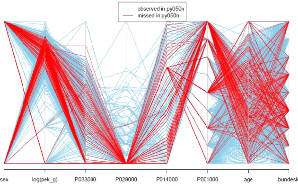
Displaying multivariate data on a graph is especially challenging, and one plot type that does it effectively is parallel coordinate plot. It represents all variables (usually scaled to fall in [0,1] interval) by parallel vertical bars, and observations corresponding to each unit are connected by lines. These plots can be produced using the R-package VIM (Templ and Filzmoser 2008), which is devoted solely to creating various visualizations of missing values in a dataset to help explore their patterns. Figure1.1 shows an example or the parallel coordinates plot, borrowed from (Templ and Filzmoser 2008).
The next two chapters describe a new systematic way to perform sensitivity anal-yses in studies with missing data by incorporating graphical displays.
Figure 1.1: An example of the parallel coordinates plot taken from Templ and Filz-moser (2008). Here, the color indicates units with missing values in the variable
py050n. We can notice that units with missing py050n have high portion of small values in the variable P033000, and P029000 = 0 for all of them. Also, some cate-gories ofP001000 and bundesld do not have any units that are missing py050n, and, for the variable pek g, nonrespondents fall only in a certain range.
Sensitivity Analysis for Partially
Missing Binary Outcomes in a
Clinical Trial with Two Arms
2.1
Introduction
Various methods of handling data with missing values have been proposed in the literature. Each one of them requires assumptions about the missingness mechanism, implicit or explicit, and full appreciation was not given to the importance of these assumptions until the pivotal work of D. Rubin in the 1970s. As described in Section
1.1, Rubin(1976) proposed to treat missingness indicators as random variables, and, since then, three missingness mechanisms were defined, MCAR, MAR, and MNAR.
Here we focus on a special but very common case when the outcome data is partially missing and a set of fully-observed predictors that explain the missingness
and the outcomes is available. Let YY = (y1, . . . , yN), where yi denotes a value of a
univariate outcome of interest for uniti, and letDDD= (d1, . . . , dN)0 be the missingness
indicator, such that di = 0 for units that are missing yi and di = 1 for units with
observedyi. LetXXX = (xi,j) be a set of predictors that consists of three nonoverlapping
subsets: predictors XXXY of the response YYY only, predictors XXXD of the missingness
indicator DDD only, and common predictors XXXY D for YYY and DDD, such that XXXY, XXXD,
and XXXY D do not overlap. The triplet (xxxi, yi, di) is assumed to be independent and
exchangeable across units, so we drop the index ito keep the notation in this section uncluttered.
Let the probability distribution of the outcomes for each unit be
f(y |xxx, θθθ) = f(y |xxxY, xxxY D;θθθ)
and the probability distribution of the missingness indicator be
f(d |xxx, y, φφφ) = f(d |xxxD, xxxY D, y;φφφ),
whereθθθandφφφare vector-parameters governing the corresponding distributions. Then, each missingness mechanism defined in Section 1.1 implies that the following holds for every unit:
• MCAR: f(d |xxxD, xxxY D, y;φφφ) =f(d |φφφ) for each φφφ and for allxxx and y. In other
words,XXXD andXXXY D are empty sets and the missingness is independent of the
response y itself.
for eachφφφ.
• MNAR: f(d | xxxD, xxxY D, y;φφφ) 6= f(d | xxxD, xxxY D;φφφ). Note that MNAR can
im-ply that there is an unobserved variable u that is associated both with the response and with the missingness indicator, such thatf(d |xxxD, xxxY D, u, y;φφφ) =
f(d | xxxD, xxxY D, u;φφφ), but, because we failed to measure u, the model for the
missingness mechanism requires conditioning on the response y itself.
Definitions of all three missingness mechanisms do not assume anything about the distribution of the outcome y, so that it does not even have to be a random vari-able (Rubin 1976). However, here we specifically focus on the situation where the distribution of the outcome is modeled using covariatesXXX.
Figure 2.1 displays graphically the three mechanisms described above. The top row shows available predictors, and the bottom row shows outcomes. Conditional dependencies are represented by lines, while the absence of a line indicates conditional independence between the corresponding variables. Here, the dependency between variables is not limited to a linear model, as in Cox and Wermuth (1993), nor does a line suggest any causal relationship, as inPearl (2009).
Many studies with missing data either use complete-case analysis (i.e., discard units with partially missing data), which is generally invalid, except in very special cases of MCAR mechanisms, or choose to analyze the data under the MAR assump-tion. The latter is usually a more sound approach than the former, especially when the MCAR assumption is contradicted by the observed data. At the same time, the MAR assumption allows us to avoid specifying a model for missingness mechanism for Bayesian or direct-likelihood inferences, assumingφφφ andθθθare distinct (see Section
(a) MCAR (b) MAR (c) MNAR
Figure 2.1: Illustration of the types of missingness mechanisms introduced in Section
1.1for a special case with univariate outcome and no missingness in covariates. Panel (a) shows that, under MCAR, xxxY D is empty and d is not related to y. Panel (b)
indicates that, for MAR, d is allowed to be associated with y through the mutual predictors xxxY D. As evident from the diagrams, MCAR assumption is a special case
of MAR . Finally, panel (c) shows that MNAR includes all cases that are not MAR.
1.1). However, although the MCAR assumption may be tested empirically (see Sec-tion1.3.1,Rubin 1976;Little 1988b), the MAR assumption is generally unassessable. Therefore, a thorough sensitivity check is necessary to assess the influence of various assumptions about the missingness mechanism on study conclusions.
Here, focusing on binary outcomes, we describe a set of convenient displays that reveal the effects of all possible combinations of the values of missing data in treat-ment and control groups on various quantities of interest, typically, on p-values and point estimates. The displays are based on the idea of “tipping-point” analysis, first introduced in Yan et al.(2009), but anticipated inMatts et al. (1997),Hollis (2002), and Weatherall et al. (2009), as a method of assessing the impact of missing data on study’s conclusions about some quantity of interest.
Tipping points of a study are defined as particular combinations of missing data values that would change the study’s conclusions. Yan et al. (2009) presented a simple way to display these combinations for studies with two arms and a binary
outcome. We enhance this initial idea by adding more details onto the display. In particular, we allow for smooth changes in quantities of interest, add the output from multiple missingness models, including MNAR, and, when available, mark historical estimates. We show how the display can help to systematize the sensitivity analyses and to demonstrate the results across different alternative models. The proposed displays enable practitioners to identify how close alternative assumptions about the missingness mechanism come to altering the study’s conclusions and, thereby, to assess the strength of the study’s evidence.
The rest of the chapter is organized as follows. Section 2.2 lays out the basics of the sensitivity analysis and the motivation for the proposed technique. Section
2.3 provides a detailed description of enhanced tipping-point displays for a binary outcome. It also includes a simulated example that demonstrates the technique and a real-data example of the recent use of the enhanced displays in a medical device clinical trial. We conclude with a discussion (Section 2.4).
2.2
Sensitivity Analyses for Studies with Missing
Data
In every empirical study plagued with missing data, researchers face a tough deci-sion about the method of handling it. The choice of the method should be justified by stating and discussing the required assumptions and, possibly, applying alternative methods to assess the extent to which the study conclusions depend on the assump-tions used. The latter constitutes the essence of asensitivity analysis for studies with
missing data, which is especially necessary if the assumptions about the missingness mechanism used in the study are unassessable, which is typical.
A sensitivity analysis consists of several steps:
• Formulating conclusions under working assumptions;
• Identifying a set of plausible alternative assumptions;
• Studying the variation in the statistical output and conclusions under these alternative settings.
Because many methods for handling missing assume a MAR mechanism, the last two steps imply weakening this assumption. However, the apparent complexity of MNAR models appears to be the primary reason why the majority of empirical research chooses to omit any sensitivity analysis altogether. Yet, in some cases, omitting it is not an acceptable option, especially when it comes to important decisions like approv-ing a drug or a medical device, or implementapprov-ing a new public policy. For example, NAS report on methods of handling missing data (NRC-Panel 2010, p. 5) made the following recommendation: “Recommendation 15: Sensitivity analyses should be part of the primary reporting of findings from clinical trials. Examining sensitivity to the assumptions about the missing data mechanism should be a mandatory component of reporting.” Other guidelines issued lately (Burzykowski et al. 2010;CHMP 2010) also stressed the need to perform sensitivity analyses that assess the impact of missing data on reported inferences and conclusions.
In spite of the rising demand, there is clearly a shortage of practical recommenda-tions as to how one should perform sensitivity analyses (Lee 2007;NRC-Panel 2010).
As pointed out in NRC-Panel (2010, p. 83), “Unlike the well-developed literature on drawing inferences from incomplete data, the literature on the assessment of sensitiv-ity to various assumptions is relatively new. Because it is an active area of research, it is more difficult to identify a clear consensus about how sensitivity analyses should be conducted.” We address this issue below and demonstrate a process of exploring MAR and MNAR models for studies with missing values in binary outcomes using enhanced tipping-point displays.
2.3
Enhanced Tipping-Point Displays for Studies
with a Binary Outcome
Tipping-point (TP) analysis was first proposed in Yan et al.(2009) to aid clinical reviewers in judging the impact of missing data in the outcome on the estimation of a treatment effect. Yan et al. (2009) constructed displays to help illustrate “tipping points” of a study, i.e., the combination of possible values of missing outcomes that would reverse the conclusion about the statistical significance of the treatment effect. These displays were further discussed in Campbell et al. (2011) as a convenient tool to reveal the results of sensitivity analysis to various deviations from assumptions made about the missing data mechanism.
Suppose that a study is conducted to estimate the effect of a vaccine (or a treat-ment) on a subsequent occurrence of a disease. A total of N study subjects are divided into treatment group or control group, and a (2×N) set of predictors XXX, along with a vector of treatment indicatorsTTT = (t1, . . . , tN)0, are completely observed
for all subjects. A vector of outcomesYYY = (y1, . . . , yN)0 indicates whether each
sub-ject developed the disease (“success”) or not (“failure”) and some subsub-jects are missing the outcome, as indicated by the vector of missingness indicatorsDDD= (d1, . . . , dN)0.
Vector YYY has four parts that correspond to observed and missing outcomes among treatment and control subjects, i.e.,YYYT
obs,YYYCobs,YYYTmis, andYYYCmis, such that
YYY = Y Y YT YYYC , YYY T = Y YYT obs Y YYT mis , YYY C = Y Y YC obs Y Y YC mis .
Let τ = E(yi | ti = 1, θθθ)− E(yi | ti = 0, θθθ) be a marginal average treatment
ef-fect, identical for all subjects i= 1, . . . , N. If the treatment is properly randomized between the subjects, an unbiased estimator of τ is
ˆ τ = X i:yi∈YYYT yi/NT − X i:yi∈YYYC yi/NC = ¯yT −y¯C, (2.1)
where NT and NC are the sample sizes for treatment group and control group
re-spectively.
For a binary outcomeYYY, an intuitive summary of missing values is the number of successes among subjects with missing outcomes, considered separately for treatment group and control group,
g(YYYTmis) = X i:yi∈YYYTmis yi =NmisT y¯ T mis, g(YYY C mis) = X i:yi∈YYYCmis yi =NmisC y¯ C mis, where NT = NT
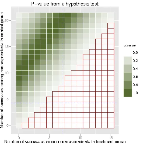
Figure 2.2: This illustration is taken from Campbell et al. (2011) to demonstrate the idea proposed in Yan et al. (2009). The horizontal and vertical axes indicate the number of successes that can potentially be observed among nonrespondents in the treatment group and the control group. Each combination is marked as either “altering the study’s conclusion” (lighter squares) or “keeping the study’s conclusion unchanged” (darker squares). The staircase region indicates the tipping points of the study.
justified by the fact that, for N i.i.d binary variables with probability of successp,
y1, . . . , yN | p∼Bern(p),
a minimum sufficient statistic (MSS) for estimating p is PN
i=1yi. Therefore, with
respect to this model, no information is lost by collapsing missing outcomes into one summary in each group. Therefore, g(YYYTmis) and g(YYYCmis) can be represented by the two axes of the enhanced TP display.
display described in Yan et al. (2009) for a binary outcome, where it results in a ma-trix of all possible combinations of the number of successes among nonrespondents in the treatment group and in the control group. Each combination is categorized based on whether the corresponding missing pattern changes, or “tips”, the conclu-sion about the estimated effect’s statistical significance. The staircase region marks the tipping points of the study, i.e., the combinations of the number of successes among nonrespondents in the treatment group (horizontal axes) and in the control group (vertical axes) that alter the conclusion about the statistical significance of the treatment effect, based on a chosen hypothesis test and a significance level. One fundamental issue with this basic depiction is that the display has no information about the likelihood of each individual combination. Therefore, unless we discover that none of possible missing data patterns change the study’s conclusion, we cannot utilize these displays to their fullest potential.
We use the initial idea of illustrating tipping points to propose a visual approach to performing sensitivity analysis. It is done by introducing the following enhancements to the displays:
• A colored heat-map that illustrates thegradual change of the quantity of inter-est, e.g., the p-value from a hypothesis test used in the study. Moreover, it can also represent the estimated treatment effects, ˆτ, the lower or upper bounds of confidence interval, or any other quantity that depends on a particular com-bination of the number of successes among nonrespondents in the treatment group and in the control group.
group, if such are available. For example, if axes represent the number of adverse events among treated and among control subjects, the ticks could indicate the numbers that correspond to the rates observed in previous studies for patients with similar demographics and medical condition.
• The results from the current modeling procedure, e.g., the posterior draws of
Y
YYmis under the chosen modelf(YYY , DDD |TTT , XXX;θθθ, φφφ).
• Most important, the posterior draws of YYYmis obtained under models with
al-ternative assumptions utilized for the sensitivity analysis. We elaborate on the last two enhancements in the following sections.
The merit of adding ticks that correspond to historical and observed values is espe-cially apparent because the practitioner may compare them with the values obtained under the primary and alternative models and, based on that, judge the sensibility of underlying assumptions.
As already mentioned, there are several quantities that may be of interest to a practitioner and could be represented by a heat-map on a TP display. First, it can represent the estimate of τ, as it varies depending on the number of successes among missing outcomes. The relationship may be expressed as follows:
ˆ
τ = y¯
T
obsNobsT + ¯ymisT NmisT
NT −
¯
yC
obsNobsC + ¯yCmisNmisC
NC (2.2)
= y¯
T
obsNobsT +g(YYYTmis)
NT −
¯
yobsC NobsC +g(YYYCmis)
NC .
Another quantity of interest is thep-value that corresponds to a test of the estimated treatment effect ˆτ. Next, we illustrate the use of enhanced TP (or ETP) displays on
a simulated example with a binary outcome and several fully-observed predictors.
2.3.1
Simulated Example with a Binary Outcome
In order to illustrate the use of ETP displays with a binary outcome, we gen-erated data for N = 100 subjects with two predictors, representing sex, F emaleF emaleF emale = (f emale1, . . . , f emaleN)0, and age in years,AgeAgeAge = (age1, . . . , ageN)0, a treatment
in-dicatorTTT = (t1, . . . , tN)0, and a partially missing outcomeYYY = (y1, . . . , yN)0 (adverse
event occurrence). Predictor F emaleF emaleF emale was simulated from Bern(0.5), and predictor
AgeAgeAge was simulated uniformly between 18 and 55 (rounding to the nearest integer). The following models were used to generate the outcomes and the missingness,
logit(pi) =2ti−0.001agei−0.1f emalei (2.3a) −0.05f emalei ·agei·I(agei >35)
−0.001f emalei·agei2·I(agei >35),
yi |pi ∼Binom(pi), (2.3b)
logit(ei) =3−0.1agei−0.5f emalei+ 0.5yi, (2.3c)
di | ei ∼Binom(ei), i= 1, . . . , N, (2.3d)
where I(·) is an indicator function. According to the notation introduced in Section
2.1, here XXXY D = (TTT , AgeAgeAge, F emaleF emaleF emale), while XXXY and XXXD are empty. As evident from
(2.3c), the missingness mechanism is MNAR. The model forpi (2.3a), the probability
of success for subject i, indicates that, although the treatment effect is positive, the success rates decline steeply for females over 35. The rapid increase in the risk of
adverse events after reaching a certain age is not an uncommon phenomenon, e.g., the risk of heart disease increases for men after the age of 45 and for women after the age of 55, the risk of having fertility issues (miscarriage, birth defects, etc.) increase sharply for women over 35.
In the simulated data, out of 100 subjects,NT = 40 were randomly assigned to the
treatment group and NC = 60 to the control group, with NT
mis = 15 and NmisC = 21
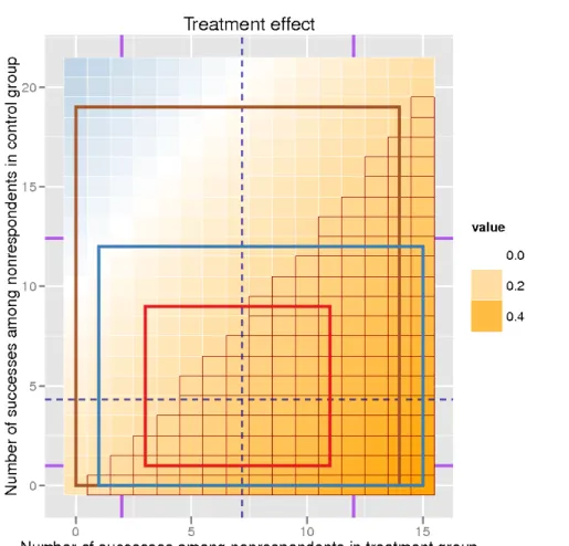
subjects missing the outcome in each group, respectively. Figure 2.3 shows the heat-map of ˆτ for the generated data set, calculated according to (2.2). If we perform the hypothesis test for the difference in proportions of successes between treatment group and control group, the results may also be shown on the ETP display. Figure
2.4 shows the heat-map of p-values and outlines the region that corresponds to a significant treatment effect based on the significance level of 0.05. Hence, the outer contour of the region indicates the tipping points of the study, i.e., the number of successes among missing outcome values in treatment group and control group that would change the conclusion of the study e.g., {1,0},{2,0},{2,1} etc. Undoubtedly, the best possible scenario for a researcher would be when the display shows no tipping points, i.e., when all combinations of missing outcomes lead to the same conclusion of the study. If it is not the case, as in our simulated example, then performing sensitivity analysis can be critical, and ETP displays can be used to guide it.
Next, we illustrate the results of three analyses performed on the simulated data. The first analysis assumes MCAR model and multiply imputes the missing out-comes based on the rates of adverse events observed among respondents, without taking into account available predictors. The last two analyses assume a MAR
Figure 2.3: ETP display for the simulated binary outcomeYYY, showing the estimated treatment effects using a heat-map. Axes represent the number of successes that could be observed among nonrespondents in the treatment group and in the control group. Each combination corresponds to a value of the estimated treatment effect ˆτ
according to (2.2). Its magnitude and sign are represented using a color palette that changes from dark blue (large negative value) to dark orange (large positive values), with white representing zero estimated effect. Note that displaying each individual value is optional (and, in fact, largely redundant), so we omit it in further displays. The axes indicate that there were 15 missing outcomes among treated subjects and 21 among control subjects. Vertical and horizontal dashed lines (in blue) correspond to observed success rate among treated and control subjects, 0.48 and 0.21.
mechanism, and multiply impute missing values from their approximate posterior predictive distributions, obtained using MICE algorithm. The second analysis uses a na¨ıve linear model for the log-odds of success to impute missing responses, i.e, logit(pi | ti, agei, f emalei;θθθ) = θ0 +θ1ti +θ2agei +θ3f emalei. The third analysis
Figure 2.4: ETP display for the simulated binary outcome YYY, showing the p-values from a chosen hypothesis test (i.e., test of the difference in proportions of successes in treated and control groups). The heat-map represents p-values obtained from the test conducted for each combination of the number of successes among treated and among control subjects. The red grid highlights combinations that result in a significant treatment effect at the 0.05 significance level, with a stair-case region indicating the tipping points of the study.
includes all the relevant interactions, as specified in (2.3a) and, therefore, is more accurate. Note that the actual details of the imputation procedure are not essential, as long as a the procedure is proper and it uses plausible assumptions about the missingness mechanism.
Table 2.1: Treatment effect on the outcomeYYY, estimated for the full dataset as well as for the observed dataset, with missing values multiply imputed using three models. For the na¨ıve and the complete models we assume MAR missingness. The results from 100 MIs are combined for each model using Rubin’s rule.
Analysis Estimated difference 95% Interval Full data 0.27 (0.09, 0.46) MCAR 0.27 (0.05, 0.48) Na¨ıve model 0.24 (-0.04, 0.53) Complete model 0.31 (0.05, 0.57)
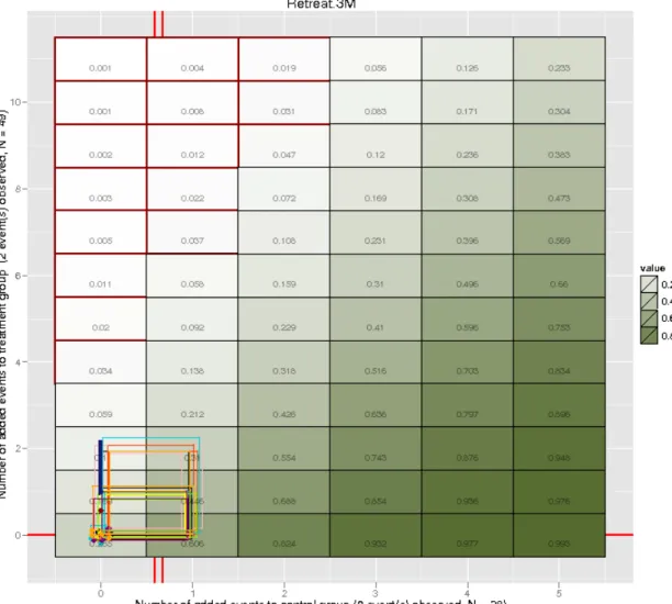
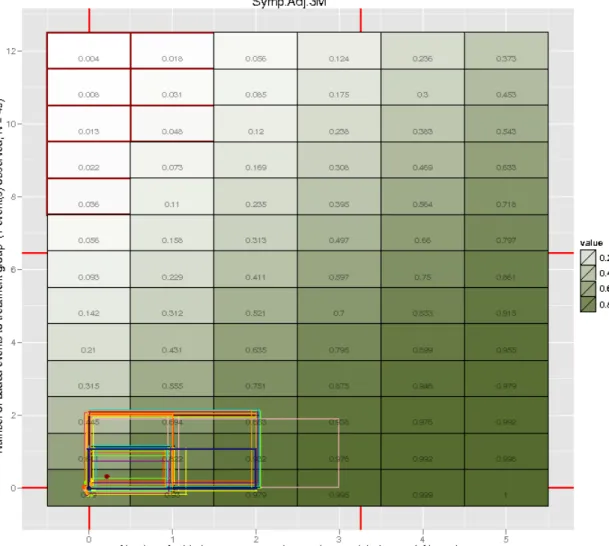
gives the estimates and corresponding 95% credible intervals obtained from 100 MIs generated for each of the three analyses and combined using the Rubin’s rule ( Ru-bin 1987; Barnard and Rubin 1999). Figures 2.5 and 2.6 show the results of the MI procedures, demonstrating different ways that the joint posterior distribution of the missing values can be summarized1. Brown, blue, and red rectangles are drawn by connecting minimum and maximum values among the imputations in each group un-der the na¨ıve, complete, and MCAR models, respectively. In Figure2.6, the (jittered) points indicate actual imputed values for each model. The corresponding contours en-circle 95% of points for each model, obtained by excluding 5% of points that have the largest Mahalanobis distance from the sample mean. These contours approximates the 95% posterior region of the joint distribution of successes among nonrespondents in the treatment group and the control group.
We also added several vertical and horizontal ticks, showing counts that corre-spond to hypothetical historical data. For example, if rates of success for subjects with similar demographics were observed to be 0.35 and 0.60 in previous studies of similar treatments, for our example they would correspond to having 2 and 12
1The R-procedure that constructs ETP displays for generated MIs can be downloaded from
Figure 2.5: ETP display showing results from three MI procedures for the simulated binary outcomeYYY. As before, the red grid highlights combinations that correspond to a significant treatment effect based on a hypothesis test for the difference between two proportions, using 0.05 significance level. In this simple version of the ETP display, the rectangles indicate minimum and maximum values among 100 imputed numbers of successes for nonrespondents in the treatment group and the control group under the na¨ıve (brown), the complete (blue), and the MCAR (red) models. Also, the display shows two vertical and two horizontal ticks (in purple), representing counts that correspond to success rates {0.35,0.60} for the treated, and {0.15,0.34} for the controls, serving to illustrate the use of data possibly available from previous studies. This version of the ETP display (with heat-map showingp-values instead of treatment effects) is used in the real-data example in Section2.3.2.
successes among nonrespondents in the treatment group, respectively.
Figure 2.6: ETP display, similar to the one shown in Figure 2.5, but more detailed. The jittered points indicate the number of imputed successes for nonrespondents in the treatment group and the control group under the na¨ıve (brown), the complete (blue), and the MCAR (red) models. Brown, blue, and red contours contain 95% of the imputations, while 5% of points with the largest Mahalanobis distance from the sample average are excluded. The contours approximate the 95% posterior region of the joint distribution of the number of successes among nonrespondents in the treated group and the control group. The results obtained from the models are somewhat different, indicating that both na¨ıve and MCAR models may not be accurate. models. In addition, Table 2.1 shows that the three models produce conflicting con-clusions regarding the significance of the effect, with the na¨ıve one indicating that there is no significant treatment effect. If additional predictors in the complete model were not relevant, we would expect similar results to be produced under both models.
Next we describe how a systematic sensitivity analysis was performed on a real data from a medical device clinical trial with multiple binary outcomes and substantial missingness, and how ETP displays were utilized to summarize it.
2.3.2
Real-data Example
So far we focused on the situation with missing values confined to a single outcome. However, the example that we present next involves a more complex problem and demonstrates how the TP analysis can be extended to the situation with missingness in more then one outcome. The data set that we use comes from a clinical trial conducted in 2008-2009 in Germany. The objective of the study was to compare the efficacy and safety of a new device for kyphoplasty, a novel treatment of vertebral compression fractures, which are the most common complications of osteoporosis, to the efficacy and safety of a traditional procedure, i.e., vertebroplasty. Both procedures involve the injection of bone cement into fractured vertebrae, with the goal to relieve pain caused by their compression and to prevent further damage.
A randomized prospective open-label study took place in four health centers across Germany. The inclusion criteria for patients required, among other things, to have up to three vertebral compression fractures in a specific region of their spines, to be at least 50 years old, and to have pain levels above a certain threshold. A total of 84 subjects were evaluated, qualified, consented and randomized to one of the two procedures, yielding 56 subjects assigned to the kyphoplasty (“treatment” group) and 28 to the vertebroplasty (“control” group).
canal, a potentially extremely serious complication that may lead to paraplegia. This endpoint, as well as the pain score, were collected 24 hours after the surgery, while the patients were still in the hospital. Both variables did not have any missing data, therefore, we will not focus on them in this section. However, a randomization-based analysis of these endpoints were highly supportive of the superiority of the kyphoplasty procedure, performed using the new device.
The study also had several secondary endpoints, including the occurrence of vari-ous adverse events within 3 months and between 3 and 12 months after the procedure, that assessed the relative safety of the new device. The following six types of adverse events were studied:
• adjacent level vertebral fracture (symptomatic and asymptomatic),
• distant level vertebral fracture (symptomatic and asymptomatic),
• retreatment (including refracture),
• death (12-month observations include deaths within 3 months).
In addition, subjects’ pain levels (0 through 10) and disability scores (0 through 100, assigned based on a completed questionnaire) were recorded during the 3- and 12-months follow-up appointments. Table 2.2 summarizes all secondary endpoints collected in the study. In addition, a set of baseline measurements was collected for each randomized patient, including:
• the number of vertebral compression fractures that required treatment (1, 2 or 3),
Table 2.2: Secondary endpoints collected in the study, indicated by “+”. Secondary Endpoint Time after surgery
At 24h 1 day to 3 months 3 to 12 months Occurrence of each of the six
adverse events
+ +
Pain level (0-10) + + +
Disability score (0-100) + +
• demographic and health data (age, sex, height, weight, BMI, physical activity level, smoking status),
• baseline pain and disability scores, duration of symptoms, health center of stay, presence of concomitant disease(s).
A considerable fraction of subjects were missing secondary endpoints. Table 2.3
reports percents of subjects in each group that had missing outcomes at each time-point. Also, the occurrence of adverse events was rare, with the range of observed rates between 0% and 2.6%, with the exception of deaths that were reported at 10.4% rate during the 12-months follow-up; the patients’ age range at the baseline was 50 to 93, therefore such a high death rate was not surprising. However, death is considered to be unrelated to the treatment assigned. In addition, a few subjects had missing-ness in one or more of the baseline covariates. In summary, the study had several major issues that complicated the analysis and required thorough attention: consid-erable fraction of non-monotone missing data in secondary outcomes that were rarely occurring events, some missingness in covariates and, moreover, small sample sizes in the treatment and the control groups. Therefore, regardless of what assumptions about the missingness we used for the initial analysis, it was essential to perform a thorough sensitivity check to these assumption, and ETP displays were utilized for
Table 2.3: Percent of subjects missing all secondary endpoints at each time-point. Treatment group Follow-up time-point
3 months, % 12 months, % 3 & 12 months, % Kyphoplasty (NT = 49)† 24 43 18
Vertebroplasty (NC = 28) 18 36 11
†7 subjects were excluded from the treatment group after randomization due to issues unrelated to the actual procedure.
(a) Continuous variables (b) Discrete variables
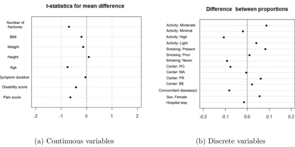
Figure 2.7: Love plots to check the balance between the treatment group and the control group produced by the randomization.
this purpose.
We start with assessing the randomization procedure and making sure it produced an acceptable balance between the treatment group and the control group. Figure2.7
contains two “Love plots”, described in Section 1.3.2(Ahmed et al. 2006), that show standardized differences between average values of baseline measurements, or between proportions for binary measurements, observed in each group. The two plots indicate an excellent balance across the two groups. We proceed with multiply imputing few missing values in baseline covariates. For that, we combine the two groups, as
justified by the randomization, but remove the outcome data. We assume MAR missingness in baseline measurements and apply the MICE algorithm to produce 100 complete data sets that will be utilized in subsequent analyses. Next, we describe the adopted assumptions about the missingness mechanism for the secondary endpoints, the procedure used for estimating the treatment effect, and the obtained results.
Questions of interest that concern secondary endpoints are whether the two treat-ments differ in the rates of adverse events as well as in the post-treatment pain levels and disability scores. As noted above, all secondary endpoints had large proportions of missingness. Therefore, in order to perform the analysis, we have to consider plau-sible assumptions about their missingness mechanism. For the initial analysis we assume the MAR mechanism and proceed to multiply impute the missing secondary outcomes using the MICE algorithm, taking into account available baseline covari-ates. For that, the outcome data