A Similarity-based Cooperative Co-evolutionary
Algorithm for Dynamic Interval Multi-objective
Optimization Problems
Dunwei Gong,
Member, IEEE,
Biao Xu, Yong Zhang, Yinan Guo, and Shengxiang Yang,
Senior Member, IEEE
Abstract—Dynamic interval multi-objective optimization prob-lems (DI-MOPs) are very common in real-world applications. However, there are few evolutionary algorithms that are suitable for tackling DI-MOPs up to date. A framework of dynamic interval multi-objective cooperative co-evolutionary optimization based on the interval similarity is presented in this paper to handle DI-MOPs. In the framework, a strategy for decompos-ing decision variables is first proposed, through which all the decision variables are divided into two groups according to the interval similarity between each decision variable and interval parameters. Following that, two sub-populations are utilized to cooperatively optimize decision variables in the two groups. Furthermore, two response strategies, i.e., a strategy based on the change intensity and a random mutation strategy, are employed to rapidly track the changing Pareto front of the optimization problem. The proposed algorithm is applied to eight benchmark optimization instances as well as a multi-period portfolio selection problem and compared with five state-of-the-art evolutionary algorithms. The experimental results reveal that the proposed algorithm is very competitive on most optimization instances.
Index Terms—Multi-objective optimization, dynamic optimiza-tion, cooperative co-evolutionary optimizaoptimiza-tion, interval similarity, response strategy.
I. INTRODUCTION
T
HERE are various multi-objective optimization problems (MOPs) with the interval characteristic in real-word applications. Each of these optimization problems generally contains more than one objective conflicting with each other, and has the interval characteristic in at least one objective and (or) constraint. One representative instance is production planning in a steel-making continuous casting-hot rolling (SCC-HR) process [1]. The process can be formulated as an MOP with the interval characteristic. For this problem, there are various uncertainties in the production process, e.g., the processing time, the production leading time, to name a few,This work was jointly supported by National Natural Science Foundation of China (61773384, 61876184, 61876185, 61873105, 61703188, 61573361, 61573362, 61503220, 61673404, 61673331, and 61763026), and National Key R&D Program of China under grant number 2018YFB1003802-01. (Corresponding author: Biao Xu and Yinan Guo.)
D. Gong, B. Xu, Y. Zhang, and Y. Guo are with School of In-formation and Control Engineering, China University of Mining and Technology, Xuzhou, 221116, China (e-mail: [email protected]; [email protected]; [email protected]; [email protected]). S. Yang is with the Centre for Computational Intelligence, School of Computer Science and Informatics, De Montfort University, Leicester, LE1 9BH, U.K. (e-mail: [email protected]).
D. Gong is also with School of Information Science and Technology, Qingdao University of Science and Technology, Qingdao, 266061, China. And B. Xu is also with School of Mathematical Sciences, Huaibei Normal University, Huaibei, 235000, China.
which are contained in such objectives as the throughput, the hot charge ratio, the utilization rate, and the additional cost, and embodied with intervals. Another typical instance is robot path planning. When planning the path of a robot, the workspace of the robot often involves various danger sources, such as fire, landmines and enemies. Given the fact that it is too expensive or even impossible to get the precise positions of these danger sources, decision-makers only know their ranges in most cases. Along this line, taking two performance metrics, i.e. the risk and the path distance, into consideration, the problem of robot path planning in the environment with uncertain danger sources can be formulated as a bi-objective optimization problem with interval parameters [2]. To illustrate the popularity of MOPs with the interval characteristic, let us investigate the reliability redundancy allocation problem. For this problem, the reliability of an individual component may be imprecise, and is generally represented with an interval, which results in an interval MOP where the reliability of the whole system and its cost are simultaneously optimized [3].
In practice, an uncertain optimization problem can also be modeled as stochastic programming [4], [5], [6] or fuzzy pro-gramming [7], [8], [9], [10] instead of interval propro-gramming. However, additional functions or information are required when formulating the problem, such as probability distribution in stochastic programming and membership functions in fuzzy programming. On the one hand, additional functions or infor-mation generally result in a complex model. On the other hand, much history information is required for describing probability distribution and membership functions, which is often hard to obtain. Furthermore, probability distribution and membership functions can be converted to intervals using the confidence level and cut set, respectively. On this circumstance, stochastic and fuzzy optimization problems can be transformed into interval optimization problems.
Interval programming is employed to tackle problems with the interval characteristic. These optimization problems gener-ally contain a number of parameters represented with intervals [11], [12], [13], [14], and the left and right endpoints or the midpoints and radius of these intervals are known a priori. It is relatively easier to obtain an interval than a probability distribution or membership function. When tackling an interval MOP, previous studies generally convert it to a deterministic single- or multi-objective optimization problem [11], [15], [16], [17]. The converted problem, however, is largely different from the original one. In addition, for the same interval MOP, different transformation approaches generally bring about
dif-ferent deterministic optimization problems. As a consequence, optimal solutions to these deterministic problems may be too diverse, which raises a big problem when selecting optimal solutions from a number of solution sets. Compared with the conversion approach, the direct approach can avoid losing valuable information and adding redundant information, thus obtaining more precise solutions.
An MOP with changing ranges of interval parameters in at least one objective and (or) constraint over time is called as a dynamic interval multi-objective optimization problem (DI-MOP). Taking the problem of robot path planning as an example, the ranges of interval parameters will change when the positions of danger sources change over time. At this point, decision-makers should rapidly adjust the robot path so as to successfully fulfill a mission.
Different from traditional dynamic MOPs (DMOPs) with precise objectives, a DI-MOP generally has objectives with in-terval values, which makes previous approaches, e.g., selecting non-dominated solutions, detecting whether an optimization problem changes or not, and responding the change, unsuitable for this problem. In addition, an algorithm is required to have the capability of obtaining a set of solutions with good performance in convergence and distribution when the problem changes. As a result, it is meaningful and greatly needed to develop efficient approaches to solving DI-MOPs.
Various studies have shown that the co-evolutionary mech-anism is beneficial to increasing the efficiency of an optimiza-tion process [18], [19]. A cooperative co-evoluoptimiza-tionary algo-rithm (CCEA) generally decomposes an optimization problem with a large number of decision variables into a number of sub-problems with a small number of decision variables, with each being optimized by a population. Each sub-population seeks the optimal solutions for a sub-problem in the corresponding search space. A complete solution, i.e., the candidate to the original optimization problem, for a sub-population is constructed by combining a best solution of the current population with the best solutions of other sub-populations at each generation. Since CCEAs can significantly reduce the search space of a sub-population which is utilized to optimize a small number of decision variables, they are efficient when solving traditional DMOPs. For example, Goh and Tan presented a dynamic competitive-cooperative co-evolutionary algorithm (dCOEA) to solve both static and dynamic MOPs, where all the decision variables are adaptively divided into a number of groups, and stochastic competitors are employed to track changing optimal solutions [20]. Two approaches to large-scale multi-objective optimization were proposed in [21] and [22]. One is to solve an MOP with many decision variables, called an evolutionary algorithm for large-scale many-objective optimization (LMEA), which divides the decision variables into distance- and diversity- related groups using a clustering approach [21]. The other is an MOEA based on decision variable analyses (MOEA/DVAs) for large-scale MOPs [22], which groups the decision variables according to the contribution of a decision variable to convergence (i.e., the distance to the PF), diversity, or both. But a large number of function evaluations are consumed before the optimization, especially for an optimization problem with a
large number of decision variables. It is not suitable for a dynamic problem, which requires an algorithm with the capability in rapidly responding to environmental changes. The proposed decomposition strategy, however, does not take the influence of changing parameters on the decision variables into consideration. Following the influence of the time scale on the decision variables, we divided all the decision variables into two groups [23], among which one contains decision variables interrelated with the time scale, and the other does not. When cooperatively optimizing the decision variables of the two groups using two sub-populations, we employed different prediction strategies to generate the initial population for different sub-populations, with the purpose of rapidly responding to the change of the optimization problem. The above methods focus mainly on real value problems and do not take interval objectives into account, hence incapable to tackle DI-MOPs. Further analyses can be found in Subsections III.C and III.D.
In addition, a non-dominated solution to an interval MOP may not be non-dominated in the scenario of a DI-MOP due to the changing ranges of interval parameters. Consequently, issues are expected to address when solving a DI-MOP, including accurately detecting the change of the optimization problem, rapidly tracking the changing Pareto front (PF), and timely providing candidates with good performance in diversity and approximation.
In this study, we focus on DI-MOPs, and a framework of dynamic interval multi-objective cooperative co-evolutionary optimization based on the interval similarity is presented to handle them. In the framework, a strategy for decomposing decision variables is first proposed, through which all the decision variables are divided into two groups according to the interval similarity between each decision variable and interval parameters. Following that, two sub-populations are utilized to cooperatively optimize decision variables in the two groups. Furthermore, two response strategies, i.e., a strategy based on the change intensity and a random mutation strategy, are employed to rapidly track the changing Pareto front of the optimization problem.
More specifically, this paper has the following four-fold contributions:
(1) Providing a cooperative co-evolutionary optimization framework for tackling DI-MOPs;
(2) Presenting strategies for grouping decision variables of a DI-MOP and detecting its change according to the interval similarity;
(3) Defining the change intensity of an optimization problem and proposing a response strategy based on it, and (4) Experimentally investigating the performance of the
pro-posed algorithm based on a set of benchmark problems and applying the proposed algorithm to a multi-period portfolio selection problem.
The rest of this paper is structured as follows. Section II provides a comprehensive review on the related work. The proposed framework of dynamic interval multi-objective cooperative co-evolutionary optimization based on the interval similarity is detailed in Section III. The experimental setting and results are reported and analyzed in Section IV. Finally,
Section V concludes the whole paper and points out several topics for future study.
II. THE RELATED WORK
A. DI-MOPs
Without loss of generality, a DI-MOP can be formulated as follows. minF(x,c(t)) = (f1(x,c1(t)), f2(x,c2(t)),· · ·, fm(x,cm(t))) s.t.x∈D⊆Rn ci(t) = (ci1(t), ci2(t),· · ·, cil(t))T, i= 1,2,· · ·, m cik(t) = [cik(t), cik(t)], k= 1,2,· · ·, l (1) where
x - an n-dimensional decision vector;
c(t) - an m-dimensional interval parameter vector;
F(x,c(t)) - an objective vector;
fi(x,ci(t)) - the i-th component ofF(x,c(t));
ci(t)
- the i-th component ofc(t), which is a vector withl components;
cik(t)
- the k-th component ofci(t), which is
an interval;
cik(t) - the left endpoint ofcik(t);
cik(t) - the right endpoint ofcik(t).
Given the fact thatci(t)is an interval vector,fi(x,ci(t))is
an objective with its value being within an interval, denoted as fi(x,ci(t))
∆
= [fi(x,ci(t)), fi(x,ci(t))], i = 1,2,· · · , m.
ci(t) generally changes over the time scale. Specially, if
ci(t) remains unchanged over time for any i, Eq. (1) will
be degraded as a traditional interval MOP [24]. In addition, if cik(t) = cik(t) is held for any i and k, Eq. (1) will be
degraded as a traditional DMOP [25]. From this viewpoint, the optimization problem formulated with Eq. (1) is an extension of previous optimization problems. As a result, studying approaches suitable for Eq. (1) is of considerable significance.
B. Dominance relation and Crowding distance based on intervals
For two solutions, x1, x2∈D, of (1), their i-th objectives
are fi(x1,ci(t)) and fi(x2,ci(t)), i = 1,2,· · · , m,
respec-tively. Limbourg and Aponte [24] defined the following order and dominance relations based on intervals.
Definition 1: Order relation. The order relation between
fi(x1,ci(t))andfi(x2,ci(t))is defined as follows.
fi(x1,ci(t))<INfi(x2,ci(t))⇔fi(x1,ci(t))≤fi(x2,ci(t))
∧fi(x1,ci(t))≤fi(x2,ci(t))∧fi(x1,ci(t))≠ fi(x2,ci(t))
(2) Otherwise, fi(x1,ci(t)) andfi(x2,ci(t))are incomparable,
denoted as fi(x1,ci(t))||fi(x2,ci(t)).
The order relation, <IN, is antisymmetric, reflexive, and
transitive. As a result, it defines a partial order relation between intervals.
Definition 2: Dominance relation based on intervals.
x1 is said to dominate x2 based on intervals, denoted as
x1≻IPx2, if and only if
∀i∈ {1,2,· · ·, m},
fi(x1,ci(t))<INfi(x2,ci(t))∨fi(x1,ci(t))||fi(x2,ci(t)),
∃i∈ {1,2,· · ·, m}, fi(x1,ci(t))<INfi(x2,ci(t))
(3)
If neither x1 dominates x2, nor x1 is dominated by x2,
x1 and x2 are non-dominated based on intervals, denoted as
x1||x2.
To obtain a diverse Pareto front, Limbourg and Aponte provided the definitions of the hyper-volume and crowding distance based on intervals [24]. Following the dominance relation and the crowding distance based on intervals, they proposed the following strategy for sorting solutions to (1). The dominance relation is first utilized to assign each solution with a unique rank. Then, for solutions with the same rank, the order relation is adopted to sort them according to their crowding distances. Finally, a random strategy is employed to sort solutions which cannot be distinguished by the above approach.
C. Interval multi-objective evolutionary optimization
Various real-world applications can be formulated as in-terval optimization problems, such as optimal dispatch of a virtual power plant [26], aircraft wing and automobile design [27], [28], and household load scheduling [29]. As a result, seeking approaches suitable for addressing interval optimization problems is of great significance in theory and applications, and among which interval analysis is one of representative tools [30].
In recent years, utilizing evolutionary algorithms (EAs) to address interval MOPs has become a rapidly growing field, and a plenty of achievements have been obtained. Roughly, there are the following two ways to handle interval MOPs with EAs. One is converting an interval MOP to a deterministic single- or multi-objective optimization problem, followed by solving the converted one using EAs. Along this line, Cheng et al. first transformed an interval MOP into a mini-max optimization problem [31]. Then, they adopted a hierarchical algorithm composed of a genetic algorithm and a nonlinear programming approach to tackle the converted problem. Jiang et al. converted an interval MOP to a deterministic MOP based on the middle point and the width of an interval [32], and further converted it to a single-objective optimization without constraints which is tackled by an EA. We converted an interval MOP with hybrid indices to a deterministic MOP using such information as the middle point and the width of an interval [15], and employed NSGA-II [33] to address the converted problem. Sahoo et al. first formulated an MOP with interval parameters, followed by converting the model to a single-objective optimization problem and solving it using an improved EA [17]. In addition, Bhunia et al. first defined the interval ordering relation between solutions to an interval MOP. Then, they transformed the interval MOP into a deter-ministic single-objective optimization problem and tackled the
converted problem using a hybrid EA [16]. Recently, focusing on an interval many-objective optimization problem, we first transformed it into a deterministic bi-objective problem, where new objectives are hyper-volume and imprecision. And then, a set-based genetic algorithm was proposed to tackle it [11].
The other is tackling interval MOPs directly by EAs based on the interval dominance relation. Keeping this line in mind, Limbourg et al. defined an interval Pareto dom-inance relation based on the interval order relation when tackling an interval MOP [24]. In addition, they proposed an imprecision-propagating multi-objective evolutionary algo-rithm (IP-MOEA) to address the interval MOP. We proposed a Pareto dominance relation based on the interval possibility and interval crowding distance [34], [35]. Using them, we selected the optimal solutions to an interval MOP. Sun et al. presented an interval Pareto dominance relation based on the lower limit of a possibility, and employed it to modify NSGA-II to cope with interval MOPs [36]. Zhang et al. evaluated solutions using a probability dominance relation [37]. Goh and Tan calculated the probability with which a solution dominates another, and compared solutions based on the probability [38]. Karshenas et al. presented anα-degree Pareto dominance to discriminate solutions to an interval MOP [39]. In addition, Dou et al. presented the scheme of the interval hesitation dominance to distinguish solutions [40]. However, different dominance relations will derive different optimal solution sets for the same interval programming problem even though the identical algorithm is adopted. It is difficult to choose a favorable solution set for users. Bearing this characteristic in mind, Sun et al. integrated previous interval dominance rules in a framework through investigating the correlations of interval dominance rules, developing a strategy to reducing a rule set and assembling the reduced rules. As a result, users can utilize the proposed ensemble dominance to handle their interval programming models. Moreover, they will free themselves from choosing an appropriate approach to assess solutions [41], [42].
D. Dynamic Multi-Objective Optimization Algorithms For a DMOP, an ideal optimization algorithm is expected to rapidly seek Pareto-optimal solutions before the prob-lem changes, and a well-designed dynamic multi-objective optimization algorithm generally has good performance in convergence and diversity.
Various studies have focused on speeding up the conver-gence and maintaining a good diversity of EAs from the following two aspects. One is developing memory-based meth-ods, which save relevant information of the current solutions, and employ it in the subsequent stages. Along this line, Goh et al. selected a number of non-dominated solutions from an archive, and re-evaluated them to obtain information for guiding the subsequent evolution [20]. In the immune clonal algorithm (ICA) for a DMOP [43], Shang et al. saved representative individuals as the initial population when the optimization problem changes, so as to accelerate the con-vergence. They also proposed an improved decomposition-based memetic algorithm in [44], and employed an archive
to store the currently best solution in each decomposition direction during the search. The helpful information offered by the archive can assist in handling neighbor sub-problems by cooperation. Azzouz et al. proposed an adaptive strategy for managing hybrid populations with memory, local search and random strategies, to effectively tackle DMOPs, which guarantees a rapid convergence and good diversity [45]. Koo et al. proposed a selective memory technique, which selects a partial retrieval based on the diversity in the decision space to maintain effective memories [46]. Recently, Chen et al. focused on DMOPs with a time-variable number of objectives in [47], and proposed a dynamic two-archive EA, denoted as DTAEA, to address them. DTAEA simultaneously maintains two co-evolutionary populations, i.e., CA and DA, during the evolution, and CA and DA will be reconstructed as the environment changes. By a restricted mating selection mechanism, DTAEA takes full advantages of complementary influences of CA and DA, with the purpose of striking the balance between convergence and diversity. Additionally, they utilized a truncation operator to retrieve the most diverse subset of memories.
The other is designing prediction-based approaches, which predict optimal solutions based on historical information when the optimization problem changes. Zhou et al. proposed a method of re-initializing a population based on prediction [48]. The method first predicts the new positions of individuals based on information collected during previous searches, and the current population is then partially or completely replaced by the predicted individuals. This method has, however, dete-riorative performance when the PS of an optimization problem changes nonlinearly over time. To improve the prediction accu-racy, a method of hybrid diversity maintenance was proposed in [49], which firstly relocates a number of solutions close to the new Pareto front by prediction based on the moving direction of each center. Following that, it employs a gradual search to generate a number of well-distributed solutions in the decision space, so as to compensate for possible inaccuracies. To maintain the diversity of a population, the rest solutions are randomly generated. Moreover, Liu et al. proposed an improved prediction model to overcome this drawback [50]. In the proposed model, two individuals are selected to guide the newly predicted individuals, which is beneficial to pre-venting them from moving toward wrong directions [48]. In addition, Muruganantham et al. presented a dynamic MOEA by utilizing a Kalman filter (KF) to predict the new PF [51], which uses less information than the strategy proposed by Zhou. Furthermore, Rong et al. proposed a multidirectional prediction (MDP) strategy to enhance the performance of EAs in addressing a DMOP. They construct multiple time series models based on historical information to predict a number of evolutionary directions. Once an environmental change occurs, a part of the population is re-initialized by the prediction model, and the rest will be randomly generated [52].
In addition to the aforementioned methods, Shang et al. combined a co-evolutionary competitive and cooperative op-eration in the immune clonal algorithm (ICA) for DMOPs to have good performance of solutions in uniformity and diversity [53], [54]. Qu et al. proposed an ensemble of multi-objective
Algorithm 1:The pseudo code of the proposed framework Input: the number of generations,g;
Output: the archive,A(t);
1 Dividing decision variables (Algorithm 2); 2 t←0,g←0 %tis the time scale; 3 Initialize sub-populations;
4 whilethe termination condition is not metdo 5 Change detection (Algorithm 3); 6 ifthe change occursthen 7 t←t+1;
8 Response to the problem change;
9 end
10 Cooperatively co-evolve sub-populations;
11 Select non-dominated solutions and store them in the archive,A(t); 12 g←g+1;
13 end 14 return A(t)
differential evolution algorithms to cope with dynamic eco-nomic emission dispatch (DEED) problems [55], [56], and the experimental results demonstrated that the proposed algo-rithm is capable in speeding up convergence and effective in handling DEED problems.
III. DYNAMIC INTERVAL MULTI-OBJECTIVE COOPERATIVE CO-EVOLUTIONARY OPTIMIZATION BASED ON INTERVAL
SIMILARITY A. The general framework
DI-MOPs have the following twofold characteristics: one is that each objective of a DI-MOP is an interval, and the other is that interval parameters in the objectives change over time. Aiming at these two characteristics, we propose a framework of dynamic interval multi-objective cooperative co-evolutionary optimization based on the interval similarity to handle DI-MOPs.
In the proposed framework, all the decision variables of an optimization problem are first decomposed according to the strategy proposed in Subsection III.C. Next, sub-populations cooperatively co-evolve with each sub-population evolving the decision variables in one group, and a complete solution is formed as described in Subsection III.F with its objective being the fitness of an individual to be evaluated. Following that, non-dominated solutions are selected, and saved in an archive. In addition, a strategy based on the interval similar-ity is employed to check whether the optimization problem changes or not, as described in Subsection III.D. If yes, the sub-populations will be re-initialized using the proposed response and perturbation strategies, respectively, as described in Subsection III.E. The above process will be repeated until a termination condition is met. The complete non-dominated solutions in the archive are finally output as the optimal solutions to the DI-MOP. Algorithm 1 provides the pseudo code of the framework.
To fulfill this task, we first define the interval similarity as follows.
B. Interval similarity
In [57], the authors provide a definition of interval similarity and its properties. The definition, however, is useless when an
interval degrades as a real value. Therefore, we extend the definition and make it also suitable for real values.
Definition 3: Interval similarity. For two intervals a =
[a, a] and b = [b, b], their similarity, denoted as s(a, b), is defined as follows. s(a, b) = la∩b max{la,lb}, max{la, lb} ̸= 0; 1−max{|a|,||bb−|,χa(||a|+|b|)}, max{la, lb}= 0, a̸= 0 or b̸= 0; 1, max{la, lb}= 0, a=b= 0. (4) wherea∩brepresents the intersection ofaandb, andla,lb, and
la∩b mean the widths of intervalsa,b, anda∩b, respectively.
max{la, lb}= 0indicates thataandbare two real values, i.e.
a=aandb=b.χis a characteristic function, with its value being 1 when ab <0, and 0 otherwise.
The value ofs(a, b)reflects the difference betweenaandb, which satisfies that0≤s(a, b)≤1, and a larger value means a smaller difference between these intervals.
In addition, we have the following observations.
(1) s(a, b)=1 if and only ifa=b , which is called complete. (2) s(a, a)=1, which is called reflexive.
(3) s(a, b) =s(b, a), which is called symmetric.
(4) Ifs(a, b) = 1ands(b, c) = 1are held, one hass(a, c) = 1, which is called transitive.
Please refer to Subsection I.A in the supplementary material for the proofs of these observations.
C. Dividing decision variables based on interval similarity For a DI-MOP, a well-designed algorithm is generally ex-pected to have good performance in convergence and diversity before the problem changes. For a solution to a DI-MOP, some of its components change over dynamic parameters, and the others remain unchanged. If we divide all the decision variables of a DI-MOP into two groups, and optimize decision variables in each group individually, the efficiency of solving the optimization problem will be improved to some degree. In [58], a differential grouping strategy is employed to discover the underlying interaction structure of the decision variables. However, the strategy cannot be directly utilized to detect the interaction between a decision variable and a parameter in a DI-MOP, especially when the parameter is an interval, due to its different characteristics with a real value. For example,
Y = [1,2]is an interval,Y−Y = [−1,1], not [0, 0]. Inspired by the study in [58], we propose a variant of the above method based on the interval similarity in this study, with the purpose of efficiently tackling a DI-MOP.
Definition 4: separable function. A function, f(x,c), is
partially additively separable, if it has the following form:
f(x,c) =
J
∑
j=1
fj(xj,cj) (5)
where fj(xj,cj) is a function associated with xj and cj,
x1,· · · ,xJ and c1,· · ·,cJ are mutually exclusive decision
vectors and parameter vectors.
f(x,c(t)), its difference, denoted as ∆f(x,c), will be as follows when xk has a disturbance ofδ.
∆f(x,c) = [∆f(x,c),∆f(x,c)],where ∆f(x,c) =f(· · · , xk+δ,· · · ,c)−f(· · ·, xk,· · ·,c), ∆f(x,c) =f(· · · , xk+δ,· · · ,c)−f(· · ·, xk,· · ·,c). (6) ∀a,[cp, cp] ̸= [c′p, c′p], δ ∈ R, δ ̸= 0, if the interval similiarity s(∆f(x,c)xk=a,cp=[cp,cp],∆f(x,c) xk=a,cp=[c′p,c′p])<1
is held,xk andcp(cp∈c)are said inseparable.
Please refer to Subsection I.B in the supplementary material for the detailed proof.
The grouping theory in [23] is a particular case as the parameter, c, is a real vector in the above theory.
In [23] and [58], only one point is utilized to group the decision variables. However, the interval is characterized by two points, the left and the right endpoints. For interval optimization problems, if only one point is employed, infor-mation provided by the other endpoint will be lost, which results in inaccuracy. Taking a function, f(x, c(t)) = c(t)x, as an example, assume that c(t)= [1,1+t] and δ=0.5. On this circumstance, ∆1=∆f(x, c(t))x=3, cp=[1,2] = [0.5,1], ∆2=∆f(x, c(t))x=3, cp=[1,3] = [0.5,1.5]. If only the left
endpoints are utilized to measure the difference between
∆1 and ∆2, we will conclude that there is no difference
according to the results of [23] and [58]. In fact, their right endpoints have a large difference. Nonetheless, based on the method proposed in this paper, their interval similarity is s(∆1,∆2)=0.5, suggesting that ∆1 and ∆2 are clearly
different. As a consequence, the method proposed in this paper can easily distinguish ∆1 and ∆2, and is more suitable for
handling interval optimization problems.
In this study, due to uncertainties and noises generally existing in the objectives, we regard xk andcp inseparable if
s(∆f(x,c)xk=a,cp=[cp,cp],∆f(x,c)
xk=a,cp=[c′p,c′p]) < θ1
, where θ1 is a threshold set in advance in the range of (0,1).
According to the above theorem, we propose the following approach of dividing all the decision variables in (1). For xk and cp(t), we first
calculate ∆f(x,c(t))xk=a,cp(t)=[cp(t),cp(t)] and ∆f(x,c(t))x
k=a,cp(t)=[c′p(t),c′p(t)] according to (6).
Following that, we obtain the similarity between the two intervals by (4), and if it is smaller than θ1, xk is
inseparable with cp(t). On this circumstance, we delete xk
from the set of decision variables, and put it into the first group. The above process is repeated until all the interval parameters are detected. In this way, we can obtain decision variables in the first group. θ1 is set according to noises and
uncertainties existing in a problem, and the larger the noises or uncertainties, the smaller the value of θ1 should be set.
For a problem, θ1 is generally set to 1. In fact, assigning its
appropriate value is difficult. Algorithm 2 provides the pseudo code of the proposed method of dividing all the decision variables.
Algorithm 2: Dividing decision variables
Input: the time scale,t; upper and lower bounds of decision variables,
upbandlowb; the number of objectives, decision variables and interval parameters,m,nandP, respectively;
Output: the groups of decision variables,g1andg2; 1 g1← ∅%g1saves decision variables inseparable withc(t); 2 g2← ∅%g2saves decision variables separable withc(t); 3 for i =1to mdo
4 forp=1to Pdo 5 fork =1to ndo
6 x(1 :n)←lowb(1 :n); 7 y(1 :n)←x(1 :n);
8 %xandymean the values of decision vector,x; 9 y(k)←0.5·(lowb(k) +upb(k)); 10 c(1 :P)←c(t)(1 :P); 11 ∆1←fi(x,c)−fi(y,c); 12 c’(1 :P)←c(1 :P); 13 c’(p)←0.5·c(p); 14 ∆2←fi(x,c’)−fi(y,c’);
15 Calculate the similarity between∆1and∆2,spk;
16 ifspk< θ1 then 17 g1←g1∪ {k}; 18 end 19 end 20 end 21 end 22 g2← {1,2,· · ·, n}\g1; 23 returng1, g2
Using the proposed strategy, all the decision variables can be divided into the following two groups: one is x1= (x11, x12,· · · , x1r), which is inseparable with interval
pa-rameters, and the other is x2= (x21, x22,· · · , x2n−r), which is
separable with interval parameters.
D. Detecting problem change based on interval similarity For a DI-MOP, if traditional approaches [25], [59], [60] are employed to detect the problem change, a predefined value associated with an objective interval, such as the left endpoint, the right endpoint, and the midpoint, is selected. However, the predefined value may not be changed as the problem varies. Let us consider the following three functions: f1(x, t) =
[1,1 +t]x, f2(x, t) = [−t,1]x, f3(x, t) = [−t, t]x,(t > 1).
When the parameter,t, varies, the left endpoint off1(x, t), the
right endpoint off2(x, t), and the midpoint off3(x, t)remain
unchanged for the same value ofx. Under this circumstance, traditional approaches have a difficulty in tackling a DI-MOP. For a solution to a DI-MOP, at least one of its objective intervals will generally vary when the optimization problem changes, and the larger the change intensity of the optimization problem, the smaller the similarity between objective inter-vals of the previous and current optimization problems. In this way, we can detect whether the optimization problem change or not. To fulfill the task, we first form a detection population at the end of each generation, which is composed of a number of individuals chosen from the current optimal solutions. Then, we calculate the similarity between objective intervals of each individual in the detection population based on the previous and current optimization problems, and obtain the average interval similarity of these individuals. Finally, we compare the average interval similarity with a threshold,
Algorithm 3: Environment detection Input: the archive,A; the number of objectives,m; Output: the results of environment detection,flag;
1 Choose u individuals from the current optimal solutions to form the detection population,det pop={p1, p2,· · ·, pu};
2 i←1;
3 whilei <=mdo 4 forj=1toudo
5 aij(t) =fi(pj,ci(t)),aij(t+ 1) =fi(pj,ci(t+ 1));
6 % Calculate the objective intervals based on the previous and the current optimization problems;
7 Calculate the similarity betweenaij(t)andaij(t+ 1),sij;
8 end 9 s¯i←1u u ∑ j=1 sij; 10 if¯si< θ2 then 11 flag←true; 12 Break; 13 else 14 flag←false; 15 i←i+ 1; 16 end 17 end 18 returnflag; TABLE I
COMPARISON RESULTS WHEN DIFFERENT STRATEGIES ARE EMPLOYED TO
DETECT THE ENVIRONMENTAL CHANGE
Function Function value
whent= 1
Function value whent= 1.5
Difference obtained by the traditional method
Similarity obtained by the proposed method
f1 (2, t) [2, 4] [2, 5] 0 0.6667
f2 (2, t) [2.2, 4] [2.3, 5] 0.1 0.6296
f3 (2, t) 4 5 1 0.8
f3 (5, t) 10 12.5 2.5 0.8
optimization problem is detected to have changed.θ2is set by
a decision-maker according to his/her preference. The more sensitive the decision-maker to the environmental change, the larger the value of θ2 should be set. On this circumstance,
the decision-maker will frequently change his/her plan once the environment changes, and has a high requirement to the algorithm so as to rapidly seeking optimal solutions. The pseudo code of the proposed method of detecting the problem change is supplied in Algorithm 3.
To compare the traditional and the proposed detection strategies, three functions, f1(x, t) = (1,1 +t)x, f2(x, t) =
(1 + 0.1t,1 +t)x, and f3(x, t) = (1 +t)x, are taken into
account. Among them, the first two are intervals, and the third one is a real value. Assume that only the left endpoints are employed in the traditional detection strategy. Table I lists the comparison results when the two strategies are employed to detect the environmental change. From this table, we can see: (1) for interval functions, f1(x, t)andf2(x, t), rows 2 and
3 demonstrate that the traditional method is low-efficient, or even useless to detect the environmental change, due to its focus on only one point and neglect of the other one. However, the proposed method detects the environment change on the interval similarity, and hence successfully detect the changes with high-efficiency.
(2) for real function, f3(x, t), both methods have a
capa-bility in detecting the environmental change. However, the proposed method is less impacted by the decision variable, suggesting its robustness. Therefore, the proposed method is also suitable for real functions.
E. Responding to problem change
Once a change of the optimization problem is detected, appropriate strategies should be employed to respond to the change. Multi-population co-evolutionary optimization can efficiently search for the feasible decision space in multiple directions and interact with each other, which makes it suit-able for addressing DMOPs. Compared with traditional sin-gle population evolutionary optimization, the multi-population counterpart generally has good performance in convergence and diversity. If all the populations respond to the change in the same way, the characteristics of different populations will be ignored, which deteriorates the performance of multi-population co-evolutionary optimization. A well-designed re-sponding strategy is generally expected to have good perfor-mance in convergence and diversity. On the one hand, aban-doning historical optimal solutions and randomly initializing a population is beneficial to the population diversity but may be time-consuming for an algorithm to converge. On the other hand, utilizing all the historical optimal solutions is helpful to converge, but may mislead the evolutionary direction when the change is severe. Furthermore, it generally results in the loss of the population diversity and falls into local optima. Therefore, seeking appropriate strategies for responding to the change is of considerable necessity.
To fulfill this task, we present a strategy for responding to changes of the optimization problem. In the proposed strategy, we initialize sub-populations corresponding to different groups using different methods. For decision variables in groups x1 and x2, they are optimized by two populations P1 and
P2, respectively. For P1, it is composed of two parts: one contains individuals which are randomly initialized in the feasible decision space to promote the diversity of P1, and the other contains those which are initialized by a prediction strategy based on the change intensity to rapidly tracking the optimal solutions to the changed optimization problem. In the following, we will detail the prediction strategy.
1) Predicting the change direction of optimal solutions : To fulfill this task, we re-evaluate solutions inA(t), the archive of complete solutions at the time scalet, and store non-dominated solutions in A0(t + 1). Then, the change direction can be
obtained as follows.
D(t+1) = CA0(t+1)−CA(t)
CA0(t+1)−CA(t)2
(7)
whereCA0(t+1) andCA(t)are the centroids ofA0(t+1)and
A(t)in the decision space, respectively.
2) Estimating the step size of the change of optimal so-lutions: We define the change intensity of the optimization problem as follows. ds(t+1) = 1 m|A0(t+1)| m ∑ i=1 |A0∑(t+1)| j=1 (1−sij) (8)
where |A0(t+1)| is the size of A0(t+1), sij refers to the
similarity between thei-th objective of the j-th individual for the previous and current optimization problems,ds(t+1)is the average dissimilarity of each objective of all the individuals.
ds(t+1) reflects the change intensity of the optimization problem, and a larger value of ds(t+1) indicates a more violent change.
Using historical information of optimal solutions, the step size of the change of optimal solutions is estimated as fol-lows.
S(t+1) =ds(t+1)
ds(t)
CA(t)−CA(t−1)2 (9)
where ds(t+1)
ds(t) means the ratio of the change intensity from
time scale t to t+1, and a larger value of dsds(t(+1)t) suggests that the change intensity at the time scalet+1 is stronger than that at time t. As a result, the step size of optimal solutions,
S(t+1), will be larger.
3) Generating new individuals: For anyp(t)∈ P1(t), its
location for the changed optimization problem is predicted as follows.
p(t+ 1) =p(t) +rS(t+1)D(t+1) +ε(t) (10) where r refers to a random value obeying the uniform distribution in [0,1].ε(t)∼N(0, σ2(t)I)is a Gaussian noise which is added to increase the probability of the re-initialized population to cover the PS of the changed optimization problem, I is an identity matrix, and σ(t) is the standard deviation of the Gaussian distribution with its expression being
σ(t) =S2(t√+1)
n .
P1 is heavily affected by interval parameters when the
op-timization problem changes. According to this characteristic, the proposed response method utilizes the interval similarity of individuals fitness before and after the change to generate the initial solutions. Due to taking full advantage of information associated with the change, the generated initial solutions can well reflect the change trend of optimal solutions, leading to a rapid convergence.
With respect toP2, interval parameters have no influences on x2. As a result, a half of individuals in P2 are randomly initialized, and the rest are initialized with the Gaussian muta-tion, shown in (11), when the optimization problem changes.
p(t+ 1) =p(t) +ε(t) (11)
F. Constructing a complete solution
When evaluating an individual of the current population, forming a complete solution by selecting a representative individual from the other population together with the current individual is of necessity. To fulfill this task, the method in [23] is adopted to construct and evaluate a complete solution. For more details, please refer to [23].
G. Complexity of the proposed algorithm
In each generation, the main difference between the pro-posed CC-IP-MOEA-IS, which is achieved by combining the proposed cooperative co-evolutionary optimization and the response strategies based on the interval similarity with IP-MOEA, and IP-MOEA lies in grouping the decision variables, detecting the environmental change, responding the change, cooperatively co-evolving each sub-population, and forming the archive. Assume that there are two sub-populations with their size of N/2 to cooperative co-evolve when tackling an
optimization problem with m(≥ 2) objectives, n decision variables, andpinterval parameters. In additional, we assume that there are k non-separable variables for each interval parameter, and letn cobe the number of representatives from the other sub-populations during the evolution, andN be the sizes of the archive. The computational complexity associated with each of the above strategies is given as follows: (1) grouping the decision variables is O(mp(n+k))[58], (2) detecting the environmental change is O(mN) in the
worst case,
(3) responding to the change is O(mN),
(4) cooperatively co-evolving all the sub-populations is
O(m(n co)2N), and
(5) forming the archive is O((2N)m)[24], [61].
The number of representatives, n co, is generally a small constant and irrelevant to the size of a sub-population. There-fore, the overall complexity of the proposed algorithm is
O((2N)m), which is the same as that of the
state-of-the-art IP-MOEA [61]. From this viewpoint, CC-IP-MOEA-IS is computationally efficient. However, if n co is set to a large value, and relevant to the size of a sub-population, CC-IP-MOEA-IS will have a high computational complexity when
m= 2.
IV. EXPERIMENTS
To evaluate the proposed algorithm, we conduct the follow-ing three groups of experiments. The first group investigates the influences of different response strategies by comparing the response strategy proposed in Section III. E with strategies A and B proposed in [25]. For the second group, its aim is to demonstrate the influences of cooperative co-evolution on an optimization algorithm. To fulfill this task, we compare IP-MOEA [24] with and without this paradigm when solving benchmark optimization instances. With the last group, we attempt to conduct a comprehensive comparison between the proposed algorithm and other five state-of-the-art ones. The implementation environment is provided as follows: Intel(R) Xeon(R) E5-2660 V3 CPU, 2.60GHz, 48GB RAM, Windows 10, MATLAB R2012a.
A. Benchmark optimization problems
To evaluate the proposed algorithm, eight new optimization problems, ZDT3DI, FDA1DI, FDA2DI, FDA4DI, FDA5DI,
and DSW1DI-DSW3DI, are constructed by modifying
previ-ous deterministic counterparts, ZDT3, FDA1, FDA2, FDA4, FDA5 [62] , and DSW1-DSW3 [63]. These problems can be scaled to any number of decision variables, and have concave, disconnected, scalable, and changeable Pareto fronts/sets. The first decision variable of each deterministic optimization prob-lem is multiplied by an interval, c1 = [0.9,1], and the
rest are multiplied by intervals associated with the time scale, ci(t) = [0.45|sin(0.5iπt)|,0.5 + 0.45|sin(0.5iπt)|]
or ci(t) = [0.45|sin(0.5πt)|,0.5 + 0.45|sin(0.5πt)|]. In this
way, the deterministic optimization problems can be converted into their interval counterparts. ci(t) changes over time, and
different decision variables have different interval coefficients, which poses a difficulty to an algorithm when tackling these
optimization problems. Therefore, these optimization prob-lems are qualified to test the capacity of an algorithm in tracking changing optimal solutions.
Please refer to Section II in the supplementary material for the detailed descriptions of them.
B. Compared algorithms and parameter settings
1) Compared algorithms and strategies: Since each sub-population in the proposed algorithm evolves using operators in IP-MOEA, it is necessary to take IP-MOEA as a compared algorithm. To investigate the efficiency of the response strategy proposed in this study, we take two state-of-the-art strategies, A and B, proposed by Deb et al. [25], into consideration for a comparative study. The three corresponding dynamic evolutionary optimization algorithms, CC-IP-MOEA-A, and CC-IP-MOEA-B, are achieved by combining the proposed cooperative co-evolutionary optimization, and the response strategies, A and B, respectively, with IP-MOEA. In addition, the other two algorithms, D-IP-MOEA-A and D-IP-MOEA-B, are obtained by incorporating the response strategies, A and B, respectively, with IP-MOEA. Finally, these two algorithms are compared with CC-IP-MOEA-A and CC-IP-MOEA-B to evaluate the performance of the proposed cooperative co-evolutionary strategy.
2) Parameter settings: In the experiments, the simulated binary crossover (SBX) and polynomial mutation are utilized with their distribution indexes of 20 to generate new offspring during the evolution. The crossover and mutation probabilities are 0.9 and 1/n, respectively, where n is the number of decision variables. For each benchmark optimization problem,
t= n1 t ⌊ τ τt ⌋
, wherent, τtandτ are the change severity and
frequency, as well as the maximal number of iterations, respec-tively. For problems ZDT3DI, FDA1DI, FDA2DI, FDA4DI,
and FDA5DI, nt = 10, τt = 50, τ = 2500, indicating that
there are fifty changes in total for each optimization problem. Each function is evaluated 10,000 times after the optimization problem changes. For problems DSW1DI-DSW3DI, nt =
2, τt = 100, τ = 2000, i.e. twenty changes are tackled for
each algorithm. Each function is evaluated 20,000 times after the change occurs.
At each generation, cooperative co-evolutionary algorithms, i.e., A, B, and CC-IP-MOEA-IS, have more evaluations than IP-MOEA. Therefore, the pop-ulation size is set to 50 for these cooperative co-evolutionary algorithms and 200 for IP-MOEA, IP-MOEA-A, and D-IP-MOEA-B, to balance their total budget in evaluation. The archive size is set to 100, and the cooperative individual rate is set to 2. Besides, the values ofθ1 andθ2 are set according
to the tolerability of a decision-maker to the problem change and the robustness of obtained optimal solutions. In this study, they are both set to 0.9. For problems with their decision variables being inseparable with interval parameters, such as ZDT3DI, FDA1DI, and FDA2DI, the decision variables are
equally divided into two groups.
We run each algorithm 30 times for each optimization problem independently, and calculate the mean and standard deviation of the two performance indicators which will be
formulated with (12) and (13). Besides, Mann-Whitney U test is adopted to show the difference of different algorithms in terms of each performance metric at the significant level of 5%.
C. Performance indicators
When evaluating a solution set obtained by an algorithm in convergence, diversity, and uncertainty, Limbourg and Aponte et al. [24] introduced such indicators as hyper-volume (H) and imprecision (I). To adapt theH andI indicators to DI-MOPs, the average value of each indicator in a period of time scales is calculated.
Definition 5: Average hyper-volume (AH). The value of
the AH metric assists in assessing the tracking ability of a Pareto optimal set obtained by an algorithm before the optimization problem changes, with its expression as follows.
AH= [AH, AH] = 1
|T|
∑
t∈T
H(X∗(t)) (12) whereT is a set of time scales with its cardinality being|T|,
X∗(t)means the obtained PS(t) at the time scale,t. The larger the value of AH of the final Pareto front is, the closer the final front is to the true one, and the better the distribution of solutions along the front is. In the experiments, the reference point is set to (1.2fmax
1 , 1.2f2max ) for DSW3DI and (5, 5)
for the rest problems, wherefmax
1 andf2max are the maximal
objectives off1 andf2, respectively.
Definition 6: Average imprecision (AI). For X∗(t), its
imprecision is calculated as follows.
I(X∗(t)) = ∑ x∈X∗(t) m ∑ i=1 (fi(x, ci(t))−fi(x, ci(t))).
The average imprecision of X∗(t) is then calculated as follows. AI= 1 |T| ∑ t∈T I(X∗(t)). (13)
AI reflects the uncertainty of a Pareto optimal set in the objective space, and the smaller the value of AI of a Pareto optimal set, the more exact the true PF(t) corresponding to the Pareto optimal set.
D. Experimental results and discussion
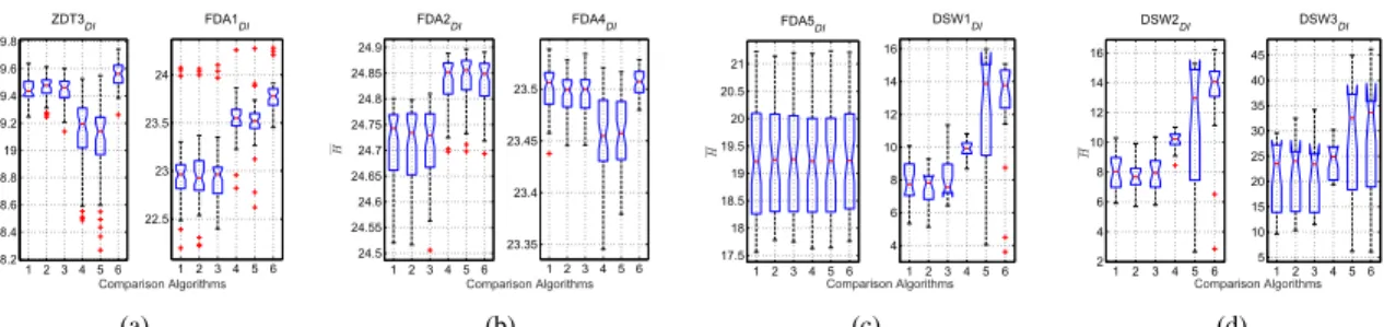
In this subsection, the proposed algorithm, CC-IP-MOEA-IS, is compared with five algorithms, IP-MOEA, D-IP-MOEA-A, D-IP-MOEA-B, CC-IP-MOEA-D-IP-MOEA-A, and CC-IP-MOEA-B. Figs. 1 and 2 depict the boxplots of the H and I indicators obtained by different algorithms when tackling the eight DI-MOPs. Tables II and III list the experimental results, where data are the average/standard deviation of AH, AI or time consumption, the boldface ones are the best among these algorithms, and those labeled by ‘*’ indicate that results obtained by the proposed algorithm are significantly different from those obtained by a comparative one.
='7', &RPSDULVRQ$OJRULWKPV * )'$', (a) )'$', &RPSDULVRQ$OJRULWKPV * )'$', (b) )'$', &RPSDULVRQ$OJRULWKPV * '6:', (c) '6:', &RPSDULVRQ$OJRULWKPV * '6:', (d)
Fig. 1. The boxplot ofH over 30 times of six algorithms on eight benchmark optimization problems. (1: IP-MOEA, 2: D-IP-MOEA-A, 3: D-IP-MOEA-B, 4: CC-IP-MOEA-A, 5: CC-IP-MOEA-B, 6: CC-IP-MOEA-IS.)
='7', &RPSDULVRQ$OJRULWKPV + )'$', (a) )'$', &RPSDULVRQ$OJRULWKPV + )'$', (b) )'$', &RPSDULVRQ$OJRULWKPV + '6:', (c) '6:', &RPSDULVRQ$OJRULWKPV + '6:', (d)
Fig. 2. The boxplot ofIover 30 times of six algorithms on eight benchmark optimization problems. (1: IP-MOEA, 2: D-IP-MOEA-A, 3: D-IP-MOEA-B, 4: CC-IP-MOEA-A, 5: CC-IP-MOEA-B, 6: CC-IP-MOEA-IS.)
1) The performance of the proposed response strategy: We first compare the two algorithms, IP-MOEA-A and D-IP-MOEA-B, on the eight benchmark problems to show the performance of incorporating response strategies A and B with IP-MOEA. Fig. 1 demonstrates that IP-MOEA-A and D-IP-MOEA-B are not better than IP-MOEA in terms of H. Especially, theH values of the former are slightly smaller than that of the latter on FDA4DI, DSW1DI, and DSW2DI,
indi-cating that there is no significant improvement in convergence and diversity after incorporating response strategies A and B into IP-MOEA. In addition, there is no significant difference in terms of AI among the three algorithms, suggesting that response strategies A and B have slightly influence on the performance of an improved algorithm. We therefore conclude the unsuitability of response strategies A and B for DI-MOPs.
Then, we compare the algorithms, CC-IP-MOEA-A and CC-IP-MOEA-B with CC-IP-MOEA-IS, which have the same cooperative co-evolution paradigm and different response strategies, A, B, and interval similarity-based, to demonstrate the performance of the three response strategies. For ZDT3DI,
FDA1DI, and FDA4DI, CC-IP-MOEA-IS is significantly
su-perior to CC-IP-MOEA-A and CC-IP-MOEA-B in terms of
H. When tackling problems DSW1DI and DSW2DI,
CC-IP-MOEA-IS achieves larger values of H than CC-IP-MOEA-A. Although CC-IP-MOEA-IS and CC-IP-MOEA-B have no significant difference in terms of the medium of H, CC-IP-MOEA-IS has the H values with a smaller fluctuation than CC-IP-MOEA-B, which highlights its strong robustness. Moreover, on DSW3DI, there is no significant difference in
terms of H among CC-IP-MOEA-IS, CC-IP-MOEA-A, and CC-IP-MOEA-B. To sum up, the proposed response strategy achieves a larger H value and a smaller fluctuation on the other problems except FDA2DI. TheAHvalue in Table II also
confirms the above observation, suggesting that the proposed
response strategy has a better capability to be combined with the cooperative co-evolution paradigm to promote the performance in convergence and diversity of an algorithm.
Additionally, CC-IP-MOEA-IS has not only smallerIvalues and stronger robustness than MOEA-A and CC-IP-MOEA-B in terms of I on ZDT3DI, FDA1DI, FDA2DI,
FDA4DI, and FDA5DI, but also its imprecise is as small
as CC-IP-MOEA-A and CC-IP-MOEA-B on DSW1DI
-DSW3DI.
From the above experimental results and analysis, we can conclude that the proposed response strategy has effectively improved in convergence and diversity of an algorithm. In addition, it significantly reduces the imprecise of the obtained optimal solution set. Hence, the proposed response strategy is more suitable for DI-MOPs.
2) The performance of the cooperative co-evolutionary paradigm: We compare the following pairs of algorithms, D-IP-MOEA-A and D-IP-MOEA-A, D-IP-MOEA-B and CC-IP-MOEA-B, with each pair having the same response strat-egy, but different evolutionary paradigm. Fig. 1 demonstrates that, CC-IP-MOEA-A and CC-IP-MOEA-B are worse than their counterparts in terms ofH on ZDT3DI and FDA4DI. In
addition, there is a slight difference among them on FDA5DI.
However, CC-IP-MOEA-A and CC-IP-MOEA-B have signifi-cantly largerH values than their counterparts on the rest five test instances, suggesting that the cooperative co-evolutionary paradigm can achieve good performance in convergence and diversity on most test cases.
We have the following observations from Fig. 2: CC-IP-MOEA-A and CC-IP-MOEA-B have largerIvalues than their counterparts on ZDT3DI, FDA4DI, and FDA5DI, but theirI
values are generally smaller than their counterparts on the rest five problems, indicating that the cooperative co-evolutionary paradigm can also improve the imprecise of an algorithm.
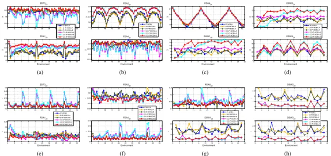
* ='7 ', (QYLURQPHQW * )'$ ', ,302($ ',302($$ ',302($% &&,302($$ &&,302($% &&,302($,6 (a) * )'$ ', (QYLURQPHQW * )'$ ', ,302($ ',302($$ ',302($% &&,302($$ &&,302($% &&,302($,6 (b) * )'$ ', (QYLURQPHQW * '6: ', ,302($ ',302($$ ',302($% &&,302($$ &&,302($% &&,302($,6 (c) * '6: ', (QYLURQPHQW * '6: ', ,302($ ',302($$ ',302($% &&,302($$ &&,302($% &&,302($,6 (d) , ='7 ', (QYLURQPHQW , )'$ ', ,302($ ',302($$ ',302($% &&,302($$ &&,302($% &&,302($,6 (e) , )'$ ', (QYLURQPHQW , )'$ ', ,302($ ',302($$ ',302($% &&,302($$ &&,302($% &&,302($,6 (f) , )'$ ', (QYLURQPHQW , '6: ', ,302($ ',302($$ ',302($% &&,302($$ &&,302($% &&,302($,6 (g) , '6: ', (QYLURQPHQW , '6: ', ,302($ ',302($$ ',302($% &&,302($$ &&,302($% &&,302($,6 (h) Fig. 3. TheHandIvalues over 30 runs versus the time instances on eight benchmark optimization problems
E. Capability in tracking the time-variant Pareto fronts The curves of H (i.e. the upper endpoint ofH) andI over 30 runs versus the time instances on the eight benchmark problems are depicted in Fig. 3. From this figure, we can obtain:
(1) For ZDT3DI, FDA4DI, and FDA5DI, two CCEAs,
i.e. CC-IP-MOEA-A and CC-IP-MOEA-B, show no better performance in both convergence and diversity than the three non-CCEAs. Nevertheless, the proposed algorithm, CC-IP-MOEA-IS, obtains the competitive H and I values along with the change of an optimization problem, indicating its excellence in tracking time-dependent Pareto fronts. Further-more, the proposed algorithm has theH andI values with a slighter fluctuation than the others, which highlights its strong robustness.
(2) For FDA1DI and FDA2DI, three CCEAs are superior
to the others no matter how an optimization problem changes, with good performance in robustness. In addition, CC-IP-MOEA-IS, which incorporates with the proposed response strategy, achieves the best performance in terms of H and
I all the time. These results reveal that CC-IP-MOEA-IS is more suitable for handling dynamic interval problems.
(3) For DSW1DI, DSW2DIand DSW3DI, which have large
feasible regions, CC-IP-MOEA-IS achieves the competitiveH
values, and is significant better than the non-CCEAs, except the first two time instances. Moreover, there is no significant difference in terms of theI values among the three CCEAs.
From the above results, we can conclude that the proposed algorithm is capable of rapidly tracking time-variant Pareto fronts as well as achieving a Pareto optimal set with good performance in convergence, diversity, and imprecision. F. Comparison analysis of algorithms
Tables II and III list the averages and standard deviations of AH andAI obtained by different algorithms on the above
eight test instances. We have the following observations in terms ofAH from Table II.
TABLE II
PERFORMANCECOMPARISONS OF DIFFERENT ALGORITHMS IN TERMS OF
AH
Problem IP-MOEA
D-IP-MOEA-A D-IP-MOEA-B CC-IP-MOEA-A CC-IP-MOEA-B CC-IP-MOEA-IS ZDT3DI 19.4401* 19.4608* 19.4406* 19.1255* 19.0730* 19.5584 0.0968 0.0871 0.1022 0.2706 0.3014 0.0935 FDA1DI 22.9704* 22.9702* 22.9629* 23.5519* 23.5085* 23.7838 0.3438 0.3686 0.347 0.2096 0.2366 0.1568 FDA2DI 24.7172* 24.7095* 24.7144* 24.8358 24.8406 24.8329 0.0727 0.0726 0.0753 0.0461 0.0458 0.0482 FDA4DI 23.4994 23.4956* 23.4961* 23.4545* 23.4582* 23.5064 0.0212 0.019 0.0194 0.042 0.0365 0.013 FDA5DI 19.2303 19.2834 19.2472 19.2267 19.2302 19.2845 1.0593 0.9789 1.029 1.0087 1.0053 0.999 DSW1DI 7.9119* 7.4199* 8.0830* 9.9035* 11.9776 12.6802 1.3337 1.1801 1.304 0.5761 4.1513 3.2384 DSW2DI 8.0367* 7.7305* 8.0613* 10.1284* 10.9399 13.1849 1.3064 1.0618 1.2896 0.633 4.627 3.0862 DSW3DI 21.6077* 21.3705* 22.0210* 24.3956 28.6406 29.6948 6.883 6.5181 7.042 3.3777 11.6022 10.3569 TABLE III
PERFORMANCECOMPARISONS OF DIFFERENT ALGORITHMS IN TERMS OF
AI
Problem IP-MOEA MOEA-AD-IP- MOEA-BD-IP- MOEA-ACC-IP- MOEA-BCC-IP- MOEA-IS
CC-IP-ZDT3DI 0.2397 0.2397 0.2415 .2779* .2812* 0.2412 -0.0202 -0.0192 -0.0206 -0.0563 -0.0642 -0.0171 FDA1DI 0.1224* 0.1228* 0.1209* 0.1061 0.1107 0.1025 0.0156 0.0154 0.014 0.0239 0.0232 0.0089 FDA2DI 0.0375* 0.0370* 0.0373* 0.0349* 0.0341 0.0336 0.0027 0.0024 0.0023 0.0024 0.0023 0.0013 FDA4DI 0.1139 0.1140* 0.1139 0.1254* 0.1272* 0.1123 0.0058 0.0053 0.0052 0.0116 0.0144 0.0039 FDA5DI 0.1308 0.1334 0.1313 0.1568* 0.1581* 0.1359 0.0083 0.0113 0.011 0.0208 0.0227 0.0131 DSW1DI 1.9086* 1.9448* 1.9085* 1.1283 1.1184 1.1461 0.2777 0.3031 0.2973 0.1345 0.1169 0.115 DSW2DI 1.9313* 1.9834* 1.8851* 1.1439 1.1392 1.1602 0.2813 0.3501 0.273 0.1734 0.1604 0.1506 DSW3DI 2.0628* 2.0640* 2.0393* 1.2564 1.2458 1.2587 0.3462 0.3029 0.2723 0.1458 0.1419 0.1132
(1) With the help of the cooperative co-evolutionary paradigm and the response strategy, CC-IP-MOEA-IS sig-nificantly outperforms the other five in terms of AH on ZDT3DI and FDA1DI. Taking ZDT3DI as an example, it is
Type I, and its true PF(t) is discontinuous. CC-IP-MOEA-IS has the AH value of 19.5584, which is better than