On the cross section of conditionally expected stock returns

WORKING PAPER SERIES

On the Cross Section of Conditionally Expected Stock Returns

Hui Guo

and

Robert Savickas

Working Paper 2003-043A

http://research.stlouisfed.org/wp/2003/2003-043.pdf

December 2003

FEDERAL RESERVE BANK OF ST. LOUIS

Research Division 411 Locust Street St. Louis, MO 63102

______________________________________________________________________________________ The views expressed are those of the individual authors and do not necessarily reflect official positions of the Federal Reserve Bank of St. Louis, the Federal Reserve System, or the Board of Governors.

Federal Reserve Bank of St. Louis Working Papers are preliminary materials circulated to stimulate discussion and critical comment. References in publications to Federal Reserve Bank of St. Louis Working Papers (other than an acknowledgment that the writer has had access to unpublished material) should be cleared with the author or authors.

On the Cross Section of Conditionally Expected Stock Returns

Hui Guo

a

and Robert Savickas

b*

October, 2003

*a _{Research Department, Federal Reserve Bank of St. Louis (411 Locust St., St. Louis, MO, 63102, E-mail:}

[email protected]); and b _{Department of Finance, George Washington University (2023 G Street, N.W.}

Washington, DC 20052, E-mail: [email protected]). We thank seminar participants at George Washington University for helpful comments. The views expressed in this paper are those of the authors and do not necessarily reflect the official positions of the Federal Reserve Bank of St. Louis or the Federal Reserve System.

On t

he Cross Section of Conditionally Expected Stock Returns

Abstract

In this paper, we use macrovariables advocated by recent authors to make out-of-sample forecast for returns on individual stocks and then sort stocks equally into ten portfolios on this proxy of conditionally expected returns. The average returns increase monotonically from the first decile (stocks with the lowest expected returns) to the tenth decile (stocks with the highest expected returns), and the difference between the tenth and first deciles is a significant 4.8 percent per year. While these portfolios pose a challenge to the CAPM, they appear to be explained by Carhart’s (1997) four-factor model. Our results indicate that the CAPM anomalies might not be attributed entirely to data snooping or irrational pricing because they are correlated with systematic movements of the macrovariables that forecast stock market returns.

Keywords: Stock Return Predictability, Cross Section of Stock Returns, Size Premium, Value Premium, and Momentum Profit.

Fama and French (2003) state that the capital asset pricing model (CAPM) of Sharpe (1964) and Lintner (1965) does not explain the cross section of stock returns. In particular, three CAPM anomalies—the size and value premiums (e.g., Fama and French [1993]) and the

momentum profit (e.g., Jegadeesh and Titman [1993])—pose a serious challenge to the existing asset pricing theories. The debate is not about the failure of the CAPM, per se, given that we have learned from the classic work of Merton (1973) that the CAPM holds only under the unrealistic assumption of constant investment opportunities. Financial economists, however, disagree on the sources of the deviations from the CAPM. For example, while Fama and French (1996) advocate Merton’s intertemporal CAPM (ICAPM) interpretation for the size and value premiums, others (e.g., Lakonishok et al. [1994] and MacKinlay [1995]) argue that they are the results of irrational pricing or data snooping. Similarly, both rational (e.g., Berk et al. [1999] and Johnson [2002]) and behavioral (e.g., Daniel et al. [1998] and Hong and Stein [1999])

explanations have been advanced for the momentum profit.

The CAPM also fails to explain the time-series variations of stock market returns since many early authors (e.g., Campbell [1987] and Whitelaw [1994]) find a weak or even negative risk-return relation in the stock market. Guo (2003a) recently suggests that the early results reflect a classic omitted variable problem: Stock market volatility is indeed positively and significantly correlated with future returns if we also include the consumption-wealth ratio proposed by Lettau and Ludvigson (2001a) in the forecasting equation.1 _{More importantly, in}

sharp contrast with Bossaerts and Hillion (1999), Ang and Bekaert (2003), and Goyal and Welch (2003), who find negligible out-of-sample stock return predictability using conventional

1 _{These results are consistent with an equilibrium model by Guo (2003b), who argues that, in addition to the risk}

premium as in the CAPM, investors also require a liquidity premium because of limited stock market participation. That is, volatility and the consumption-wealth ratio forecast stock market returns because they are proxies for the

forecasting variables, Guo (2003a) shows that volatility and the consumption-wealth ratio predict stock market returns out of sample. These results suggest two things: (1) Although important, stock market volatility by itself does not provide an adequate description for the dynamic of stock market returns and (2) investment opportunities change over time.

In this paper, we investigate, as conjectured by Fama (1991), whether there is a link between the CAPM anomalies and the time-series stock return predictability. In particular, we try to understand the sources of variations of the cross-sectional average returns by forming portfolios on conditionally expected returns. Our approach is directly motivated from recent theoretical works by Campbell (1993), Berk et al. (1999), Johnson (2002), Gomes et al. (2003), Zhang (2003), and Dai (2003), among others, who argue that the CAPM anomalies are related to the cross section of conditional returns. For robustness, we do not impose any restrictions on the structure of the risk factors; instead, we assume that, as in Ferson and Harvey (1999), some predetermined macrovariables are able to capture a significant portion of variations of expected returns for individual stocks. As mentioned above, the cross-sectional variations of returns on portfolios sorted on characteristics such as capitalization and the book-to-market ratio are consistent with many alternative hypotheses, e.g., irrational pricing and data snooping, in addition to ICAPM. In contrast, our approach of sorting stocks on the sensitivity to

predetermined macrovariables is not vulnerable to these criticisms and thus provides a powerful test for the CAPM versus ICAPM.2 _{This is the main motivation of our paper.}

risk and liquidity premiums, respectively. The forecasting ability of the consumption-wealth ratio is also consistent with other rational pricing models, e.g., the habit formation model by Campbell and Cochrane (1999).

2 _{Jagannathan and Wang (1996), Lettau and Ludvigson (2001b), Ang and Chen (2003), and Petkova and Zhang}

(2003), among others, argue that the CAPM might hold conditionally but not unconditionally because beta might co-vary with the equity premium. However, this issue is much less pronounced if relevant at all for the portfolios analyzed in this paper because under the null hypothesis of the CAPM, sorting on conditionally expected returns is equivalent to sorting on conditional beta. Also, Lewellen and Nagel (2003) argue that the covariances between betas and the equity premium have very small effects on asset pricing.

At the end of a quarter, we make a one-quarter-ahead out-of-sample forecast for each stock using the macrovariables advocated by Lettau and Ludvigson (2001a) and Guo (2003a). Stocks are then sorted on this forecast equally into ten portfolios, ranging from the portfolio of stocks with the lowest expected returns (first decile) to the portfolio of stocks with the highest expected returns (tenth decile), and the portfolios are held over the next two quarters.3 Our forecasting variables provide a decent description for the time-series variations of individual stocks: The cross-sectional average of the adjusted R-squared has a sample mean of 8.7 percent over the period 1954:Q3 to 2002:Q4. More importantly, the average portfolio returns increase monotonically from the first decile to the tenth decile and the difference between the two is a significant 4.8 percent per year. Although substantially attenuated, the return on our strategy of buying expected winners and selling expected losers remains statistically significant after we control for past raw returns. The momentum strategies sorted on predicted returns and raw returns, respectively, are thus related but distinct phenomena possibly because loadings on the other risk factors also affect expected returns. Indeed, while the portfolios formed on predicted returns pose a challenge to the CAPM, they are significantly correlated with and thus better explained by the Fama and French (1993) three-factor model augmented by a momentum factor, as advocated by Carhart (1997). Our results are consistent with an ICAPM interpretation for the CAPM anomalies: We cannot attribute them entirely to data snooping or irrational pricing because they are correlated with systematic movements of macrovariables that forecast stock market returns.

Our paper is closely related to Guo (2002), who estimates a variant of Campbell’s (1993) ICAPM using the same forecasting variables as in this paper and finds that it explains the value

3 _{The difference between returns on the tenth and first deciles is two standard deviations above zero for the holding}

premium and the momentum profit significantly better than the CAPM does. In this paper, however, we address the same issues from a different perspective, namely, uncovering the sources or mechanisms of “abnormal” returns at the individual stock level. Our paper is also closely related to Chordia and Shivakumar (2002; CS, hereafter), who argue that the momentum is completely explained by the cross-sectional variations in the expected component of past returns. However, unlike CS, we find that the momentum is related to, but not completely explained by, the cross-sectional variations of conditionally expected returns. This difference mainly reflects the fact that we use quarterly data and, especially, that our forecasting variables appear to have better out-of-sample predictive power than conventional variables used in CS, including the dividend yield, the term premium, the yield on the three-month Treasury bill, and the default premium.4 _{Our results thus should provide an additional insight on the relation}

between the momentum and conditionally expected returns.5 Recent authors, e.g., Brennan et al. (2003) and Campbell and Vuolteenaho (2003), have also stressed the importance of the

connection between the time-series and the cross-sectional variations of stock returns. The remainder of the paper is organized as follows. We briefly discuss theoretical

motivations in Section I and explain the data in Section II. The empirical results are presented in Section III and some concluding remarks are offered in section IV.

4 _{We use quarterly data because the consumption-wealth ratio is reliably available on a quarterly basis. More}

importantly, stock returns exhibit stronger predictability in quarterly data than in monthly data, as used by CS. However, we find that the momentum profit obtained from quarterly return data is very similar to that obtained from monthly return data.

5 _{Cooper et al. (2003) show that the results of CS are sensitive to microstructure concerns. Also, Chen (2002) and}

Griffin et al. (2003) find that the forecasting variables in CS do not explain the momentum in multi-factor models. In contrast, our results appear to be realistic: Given that the momentum is only one of the priced risk factors, a stock might have relatively high expected returns because of its relatively high loadings on stock market returns, for example. Indeed, we find that the market risk, the size and value premiums, and the momentum all make positive contributions to the trading profit of buying expected winners and selling expected losers. In other words, the double-sort analysis in CS does not provide a test for the momentum profit and thus should be interpreted with caution.

I.

Time-Series and Cross-Sectional Expected Stock Returns

From the classic work of Merton (1973), we know that a hedge for time-varying investment opportunities may have important effects on asset prices. In this section, we use a variant of Campbell’s (1993) discrete-time ICAPM to briefly discuss the relation between the time-series and cross-sectional expected stock returns, which we investigate in this paper.

Suppose that x_t is a K-by-1 vector of variables that forecasts real stock market return r_{m t, 1+} .6 For simplicity, we assume that x_t+1 and r_{m t, 1+} jointly follow a first-order vector auto-regressive process: (1) , 1 ₀ , ₁ 1 m t m t t t t r r A A x x ε + + +     = + +         .

where A₀is a (K+1)-by-1 vector of intercepts, Ais a (K+1)-by-(K+1) matrix of slope parameters, and ε_t+1 is a (K+1)-by-1 vector of shocks. We also assume that excess return on stock i, r_{i t, 1+} −r_{f t, 1+} , follows a stochastic process

(2) r r B B r x i t f t i i m t t i t , , , , +1− +1 = 0+

L

NM

O

QP

+η +1,

where B_i0 is the intercept, B_i is a (K+1)-by-1 vector of slope parameters, and η_{i t, 1+} is the shock to the return on stock i at time t+1. Campbell (1993) shows that, if stock returns and consumption are jointly log-normal and homoskedastic, expected return on stock i is determined by its conditional covariances with the state variables x_t+1 and r_{m t, 1+} :

(3) E r_{t i t} r_{f t} E_t i t E p t k i t k t k K ( _{, ,} ) , , , + + + + + = + − + =

∑

1 1 1 2 1 1 1 1 2 η _{η ε} ,

6 _{Campbell’s ICAPM indicates that we should use real stock market returns as a risk factor, while we usually use}

excess stock market returns as the risk factor in the CAPM. However, given that the real risk-free rate is very low and very smooth in the data, this difference has very small effects on asset pricing.

where 2 , 1 2 i t η ₊

is the adjustment for Jensen’s inequality and p_kis the risk price for factor k, which is a non-linear function of structural parameters, e.g., the relative risk aversion coefficient, and slope parameters A, as in equation (1). It should be noted that, as shown by Guo (2002), equation (3) also holds under general conditions, for example, when conditional stock market volatility is a linear function of x_t or stock returns follow an ARCH process.

Campbell’s ICAPM suggests that, in addition to a stock market return, risk factors should also include variables that are related to future investment opportunities, e.g., mean and variance of future stock market returns. If neither stock market returns nor volatility is predictable, it is straightforward to verify that Campbell’s ICAPM is reduced to the static CAPM, in which a stock market return is the only priced risk factor. Therefore, the CAPM is unlikely to price the cross section of stock returns since there is mounting evidence of time-varying stock market returns and variance.7 This implication motivates our empirical test of the CAPM using portfolios sorted on conditionally expected returns, which we discuss below.

In the empirical analysis, we exploit the ICAPM restriction that stock returns are

predictable (equation (2)) because the conditional covariances with risk factors change over time (equation (3)). For example, in the special case of the CAPM, there is a linear relation between conditional stock market returns and variance:

(4) E r_{t m t} r_{f t} E_t m t E p t m m t ( _{, ,} ) , , +1− +1 + + = + 1 2 1 2 2 η _η .

This relation, which was first advocated by Merton (1980), justifies the use of realized volatility as a forecasting variable for stock market returns and has been intensively investigated in the

7 _{However, Zhang (2003) shows that time-varying investment opportunities might have small effects on the cross}

empirical literature. For individual stocks, the CAPM suggests that conditional stock returns are a linear function of conditional covariances with stock market returns:

(5) E r_{t i t} r_{f t} E_t i t E p t m i t m t ( _{, ,} ) , , , +1− +1 + + = + + 1 2 1 1 2 η _{η ε} .

Harvey (1989), among others, has investigated whether stock returns are predictable because of the time-varying covariances with stock market returns.

Conditional covariances are usually difficult to measure, and, more importantly, financial economists have not agreed on which factors should be included in equation (3) yet. However, Campbell’s ICAPM suggests that we can circumvent these difficulties by using out-of-sample forecasts based on equation (2) as a proxy for conditionally expected returns. In particular, we sort stocks on conditionally expected returns into ten portfolios, ranging from the portfolio of stocks with the lowest expected returns (first decile) to the portfolio of stocks with the highest expected returns (tenth decile). Under the null hypothesis of the CAPM, as in equation (5), sorting stocks on expected returns is theoretically equivalent to sorting stocks on conditional beta, as in Fama and MacBeth (1973), for example. The cross-sectional variations of the average returns on these portfolios should thus be explained by their covariances with stock market returns. As mentioned in footnote 2, recent authors argue that we might reject the unconditional CAPM even though it holds conditionally because beta may co-move with the equity premium. For example, Lettau and Ludvigson (2001b) argue that value stocks are riskier during economic downturns than during economic upturns. This criticism, however, should be much less

pronounced for our portfolios because they are directly sorted on betas under the null hypothesis of the CAPM. Alternatively, if the value and size premiums, for example, are also priced factors, a stock has a relatively high expected return also because it has relatively high covariances with these additional risks. In this case, the returns on the portfolios sorted on conditionally expected

returns also reflect the dispersion of loadings on the other risk factors and thus cannot be explained by the CAPM.

Many early authors, e.g., Fama and French (1993), have tested the CAPM using

portfolios sorted on various characteristics, such as capitalization and the book-to-market value ratio. In particular, Fama and French (1993) and many others find that the resulting portfolio strategies, namely, the size premium (SMB) and the value premium (HML), exhibit statistically and economically significant deviations from the CAPM.8 However, MacKinlay (1995), among others, argues that we should be cautious about these empirically motivated anomalies because they are vulnerable to the criticisms of data snooping. More importantly, while Fama and French (1996) advocate an ICAPM interpretation for the size and value premiums, the characteristic-based risk factors are admittedly ad hoc; for example, the CAPM anomalies might also be consistent with irrational pricing (e.g., Lakonishok et al. [1994]). In contrast, sorting stocks on conditionally expected returns is directly motivated from ICAPM and thus not vulnerable to the criticisms of data snooping and irrational pricing; therefore, it should provide a powerful test for the CAPM versus ICAPM. Our empirical specification is also consistent with the theoretical works by Berk et al. (1999), Johnson (2002), Gomes et al. (2003), Zhang (2003), and Dai (2003), among others, who attribute the CAPM anomalies to the cross-sectional variations in

conditionally expected returns.

8 _{The size premium is the return on a portfolio that is long in small stocks and short in big stocks. The value}

premium is the return on a portfolio that is long in stocks with high book-to-market value ratios and short in stocks with low book-to-market value ratios. Basu (1977) and Banz (1981) have also stressed the size effect, and Graham and Dodd (1934) have analyzed the value effect.

II.

Data

As in Guo (2003a), we use the consumption-wealth ratio, realized stock market variance, and the stochastically detrended risk-free rate to forecast stock returns. As mentioned in footnote 1, the forecasting ability of the consumption-wealth ratio and realized stock market variance is consistent with rational pricing models. Also, Patelis (1997) suggests that variables such as the stochastically detrended risk-free rate forecast stock returns because these variables reflect the stance of monetary policies, which have state-dependent effects on real economic activities through a credit channel (e.g., Bernanke and Gertler [1989]). To be consistent with Campbell’s ICAPM, we also add excess stock market returns as an additional forecasting variable, as in equation (2); however, we obtain very similar results if we drop it from the forecasting equation.

There is, however, an important conceptual issue of using the consumption-wealth ratio—the error term from the cointegration relation among consumption, wealth, and labor income—as a forecasting variable. In particular, following the early authors, we use the consumption-wealth ratio estimated using the full current vintage data, although practitioners might need to estimate the cointegration vector using information available at the time of

forecast and consumption and labor income data are subject to revisions. This approach, which is consistent with rational expectations models, is appropriate for the purpose of this paper, in which we address the question “Are Expected Excess Returns Time-Varying” (Lettau and Ludvigson [2003]). Moreover, investors may obtain the same information from alternative sources; for example, Guo and Savickas (2003) show that a measure of the (value-weighted) idiosyncratic volatility, which is available in real time, has forecasting abilities that are very similar to the consumption-wealth ratio. Consistent with Guo and Savickas, we also find

qualitatively the same results in this paper by using their measure of the idiosyncratic volatility instead of the consumption-wealth ratio as a forecasting variable.9

Because the consumption-wealth ratio is reliably measured only on a quarterly basis, we use quarterly data over the period 1952:Q2 to 2002:Q4, the longest sample available to us when this paper was first written. The issue of data availability aside, we believe that quarterly data are more appropriate for the purpose of this paper than monthly data because stock returns exhibit stronger predictability at the quarterly frequency. We obtain the consumption-wealth ratio from Martin Lettau at New York University, and Lettau and Ludvigson (2001a, 2003) provide detailed discussion on this variable. Following Merton (1980), among many others, realized stock market variance is the sum of the squared deviation of the daily excess stock return from its quarterly average in a given quarter.10 _{We use the daily stock market return data constructed by Schwert}

(1990) before July 1962 and use the value-weighted daily stock market return data from the Center of Research for Security Prices (CRSP) thereafter. The daily risk-free rate is not directly available, but we assume that it is constant within a given month and the monthly risk-free rate is also obtained from the CRSP. The stochastically detrended risk-free rate is the difference

between the risk-free rate and its average over the previous four quarters: The quarterly risk-free rate is approximated by the sum of the monthly risk-free rate in a given quarter. We aggregate the CRSP monthly value-weighted stock market return into quarterly data through compounding and the excess stock market return is the different between stock market returns and the risk-free rate. Following exactly Guo and Savickas (2003), we use 500 common stocks of the largest capitalization and use the Fama and French three factors to adjust for systematic risks in the

9 _{We focus mainly on the consumption-wealth ratio because, as mentioned above, it is a theoretically motivated}

variable. In contrast, the idiosyncratic volatility forecasts stock returns because of its co-movements with the consumption-wealth ratio, and such a link has not been well understood. Also, the consumption-wealth ratio is available in a longer sample than the idiosyncratic volatility.

construction of the idiosyncratic volatility, which is available over the period 1963:Q3 to 2002:Q4.

Equation (6) shows that, consistent with Guo (2003a), the consumption-wealth ratio (CAY), realized stock market variance (MV), and the stochastically detrended risk-free rate (RREL) are strong predictors of excess stock market returns (ER) with the adjusted R-squared of over 15 percent for the period 1952:Q3 to 2002:Q4.11 _{Guo (2003a) also shows that these}

macrovariables drive out the conventional predictive variables, such as the dividend yield, the default premium, and the term premium out of the forecasting equation.

(6) ER(t+1) = Constant + CAY(t) + MV(t) + RREL(t) + ER(t) + SHOCK(t+1) -1.387*** 2.456*** 4.946*** -4.611** 0.009

(-5.513) (5.563) (3.125) (-2.246) (0.126) Sample: 1952:Q3-2002:Q4, Adjusted R-squared: 0.156

Similarly, equation (7) shows that, consistent with Guo and Savickas (2003), the idiosyncratic volatility (IV) is also a strong predictor of stock market returns when combined with stock market variance.

(7) ER(t+1) = Constant + IV(t) + MV(t) + RREL(t) + ER(t) + SHOCK(t+1) 0.030*** -3.614*** 9.894*** -5.322** 0.009

(3.492) (-5.539) (4.582) (-2.485) (0.126) Sample 1963:Q4-2002:Q4, Adjusted R-squared: 0.133

10 _{Following Campbell et al. (2001), among others, we adjust stock market volatility downward for 1987:Q4 because}

the 1987 stock market crash has a confounding effect on our volatility measure.

11 _{Heteroskedasticity-corrected t-statistics are in parentheses. *** and ** denote significant at the 1 and 5 percent}

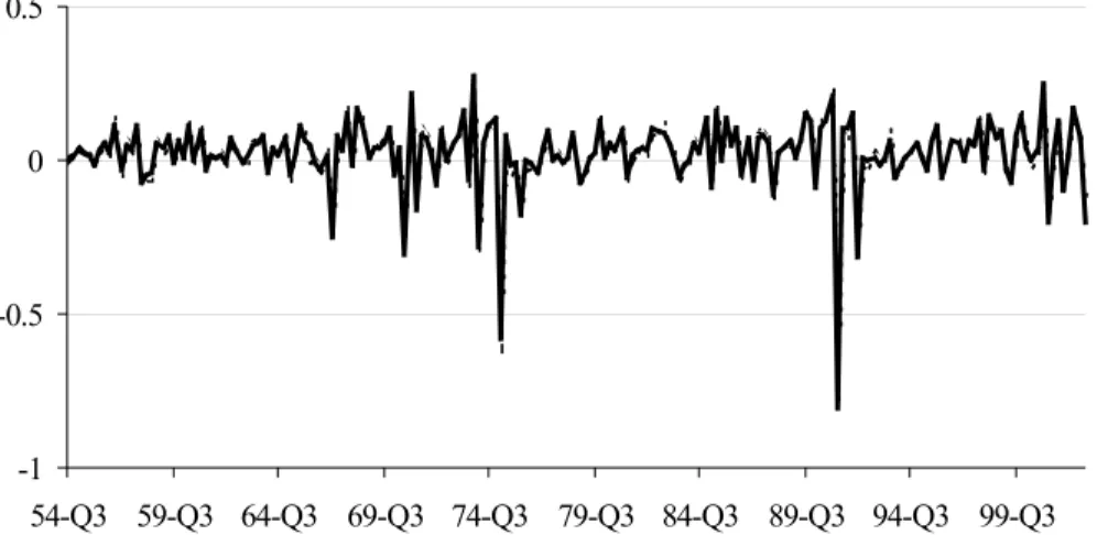
Given its similarity to the momentum strategy, we follow Jegadeesh and Titman (1993), among many others, in forming portfolios sorted on conditionally expected returns. In particular, we use all common stocks listed on the New York Stock Exchange (NYSE) and the American Stock Exchange (AMEX) in the CRSP files. However, unlike the early authors, who construct the momentum portfolios using monthly returns, we must rely on quarterly returns for the reason mentioned above. We aggregate the CRSP monthly stock returns into quarterly returns through compounding: If a stock has a missing monthly return in a quarter, we set the quarterly return to be a missing value. Therefore, it is important to verify that the momentum based on quarterly returns is similar to the momentum based on monthly returns. To investigate this issue, at the end of each quarter, we sort stocks into ten portfolios on returns in the previous two quarters, ranging from the portfolio of stocks with the lowest past returns (first decile) to the portfolio of stocks with the highest past returns (tenth decile). These portfolios are then held over the next two quarters. These specifications mimic the 6-month formation period and 6-month holding period, which are commonly used in the momentum literature. Table 1 provides summary statistics of the equal-weighted returns on portfolios formed on past returns. Over the period 1954:Q3 to 2002:Q4, the average returns increase monotonically from past losers (column 1) to past winners (column 10) and the difference between the tenth and first deciles (column 10-1) is a significant 9.2 percent per year. This number is very close to the momentum profit of 8.8 percent obtained from monthly return data.12 We find very similar results in two subsamples as well. Moreover, Figure 1 shows that the momentum profit constructed from quarterly return data (dashed line) moves very closely with the momentum profit constructed from monthly return data, and their

correlation coefficient is 0.98. Therefore, using quarterly data should not affect our inference about the momentum in any qualitative manner.

III.

Empirical Results

A. Cross Section of Conditionally Expected Stock Returns

At the end of quarter t, we run an ordinary least-squares (OLS) regression of returns for each stock using the four predetermined variables, namely, the consumption-wealth ratio, realized stock market variance, the stochastically detrended risk-free rate, and past stock market returns, as in equation (2). Following CS, we require at least two years of observations in the regression. Given that our regression is intended to capture the systematic movement of

individual stock prices, we exclude returns of 100 percent and above from the regression because these returns are driven mainly by idiosyncratic shocks. It should be noted that we do not

exclude these returns for holding periods. We also allow the forecasting sample to increase over time because, as shown by Guo (2003a), our forecasting variables have a stable relation with stock returns and the longer sample allows us to obtain more reliable out-of-sample forecasts. However, we find qualitatively the same results using a rolling sample of fixed number of observations, as in CS.

Figure 2 plots the cross-sectional average of the adjusted R-squared through time. It has a sample mean of 8.7 percent over the period 1954:Q3 to 2002:Q4, indicating that our forecasting variables are able to capture a substantial portion of predictable variations in individual stock returns. However, the adjusted R-squared tends to decrease over time. For example, its average is 11.1 percent in first-half sample 1954:Q3 to 1978:Q4, compared with 6.3 percent in second-half

12 _{Following the early authors, e.g., Jegadeesh and Titman (1993), we use a 6-month formation period and a 6-month}

sample 1979:Q1 to 2002:Q4. There are two possible explanations for the downward trend in Figure 2. First, Guo (2003a) shows that stock market returns have become less predictable in recent periods. For example, in the regression of equation (6), the adjusted R-squared is 25.0 percent in first-half sample 1954:Q3 to 1978:Q4, compared with 9.1 percent in second-half sample 1954:Q3 to 1978:Q4. Second, Campbell et al. (2001), Goyal and Santa-Clara (2003), and Guo and Savickas (2003), among others, have documented an increasing trend in the

idiosyncratic stock volatility and we find that the idiosyncratic volatility constructed by Guo and Savickas is negatively and significantly correlated with the cross-sectional average of the R-squared. Overall, if we use the existing literature as a benchmark, our forecasting variables provide a decent description for conditional stock returns.13

We use the fitted value, B$_, r , x

i t m t

t

L

NM

O

QP

, as a proxy for conditionally expected returns at quarter t+1 for stock i.14 We then sort stocks equally into ten portfolios on this forecast, ranging from the portfolio of stocks with the lowest expected returns (first decile) to the portfolio of stocks with the highest expected returns (tenth decile). These portfolios are held over the next two quarters and Table 2 presents the summary statistics for the equal-weighted returns on the portfolios formed on conditionally expected returns. Over the period 1954:Q3 to 2002:Q4, the average portfolio returns increase monotonically from the first decile (column 1) to the tenth decile (column 10) and the difference between the two (column 10-1) is a significant 4.8 percent per year. We document very similar patterns in the two subsamples of Table 2. These results confirm that the cross-sectional variations of stock returns are related to the time-series

data through compounding.

13 _{Over the period January 1953 to December 1994, CS report an average adjusted R-squared of 3.5 percent. It is 9.8}

percent in our data for a similar period 1954:Q3 to 1994:Q4.

14 _{Following CS, we do not include the intercept,}$

,

predictability of stock returns. Interestingly, compared with the momentum sorted on past

returns, as reported in Table 1, the momentum sorted on expected returns has a smaller mean but a higher t-value and thus a higher Sharpe ratio. This is because, as shown in Figure 3, the latter (solid line) is much less volatile than the former (dashed line).

B. CAPM

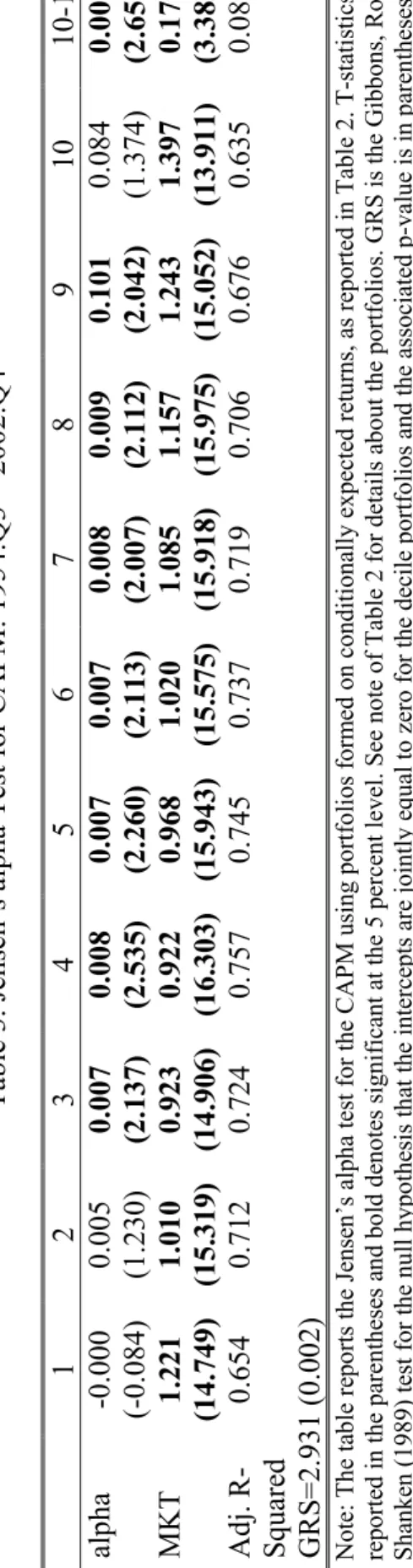
In this subsection, we investigate the main issue of this paper: Whether the CAPM explains the cross-sectional variations of returns on portfolios formed on conditionally expected returns. Table 3 presents the results of Jensen’s alpha test, in which we run an OLS regression of a portfolio return on constant and excess stock market returns. Under the null hypothesis that the CAPM is the true model, the intercept should not be statistically different from zero. Otherwise, a hedge for time-varying investment opportunities is also an important determinant of asset returns—or we need an ICAPM to explain the cross section of stock returns.

Table 3 shows that stock market return (MKT) is highly significant in the regressions and accounts for 60-70 percent of variations of portfolio returns. Interestingly, except for the first and second deciles, market beta does increase monotonically—from the third decile to the tenth decile—and it makes a significantly positive contribution to the trading profit of buying expected winners and selling expected losers (column 10-1). This pattern confirms that a stock has a relatively high return because of it relatively large covariance with stock market returns. However, the CAPM fails dramatically to explain the portfolio returns: Seven of ten portfolios have intercepts that are significantly larger than zero at the 5 percent level. Also, the trading profit of buying expected winners and selling expected losers is a significant 3.6 percent per year, after being adjusted for stock market risk. The last row reports the Gibbons et al. (GRS,

1989) test that the intercepts of the decile portfolios are jointly zero and the null hypotheses is rejected at the 1 percent significance level. Therefore, our results provide an overwhelming rejection for the CAPM and highlight the importance of intertemporal pricing.

C. Fama and French Three-Factor Model

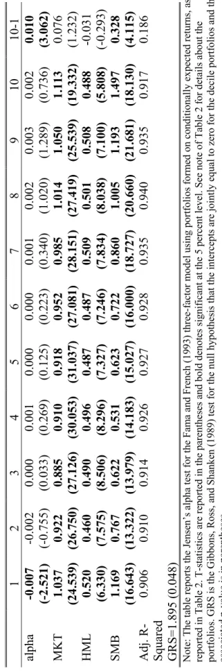
In this subsection, we investigate whether the Fama and French three-factor model explains returns on portfolios formed on conditionally expected returns.15 Table 4 presents the Jensen’s alpha test for the Fama and French three-factor model and we observe some significant improvements in explaining returns on the ten portfolios formed on conditionally expected returns. First, in addition to a stock market return, the other two factors, the value premium (HML) and the size premium (SMB), are also significantly correlated with returns on all decile portfolios. Second, the adjusted R-squared increases substantially from about 70 percent in Table 3 to over 90 percent. Third and more importantly, the intercepts are statistically insignificant except the first decile, which is significantly negative. Therefore, the size premium (SMB) and value-premium (HML) help explain the cross section of conditionally expected returns. This result should not be too surprising because, as pointed by Berk (1995), the capitalization and the book-to-market ratio incorporate information about future returns. Our results suggest that we might not attribute the value and size premiums to data snooping or irrational pricing because they are correlated with returns on the portfolios that track investment opportunities.

Nevertheless, the Fama and French three-factor model does not fully account for the cross-sectional variations of the portfolio returns since the difference between the tenth and first

15 _{We obtain the size and value premiums as well as the momentum factor used in the next subsection from Ken}

deciles is still a significant 4 percent per year in Table 4. Also, the GRS test rejects the Fama and French three-factor model at the 5 percent significant level.

D. Four-Factor Model

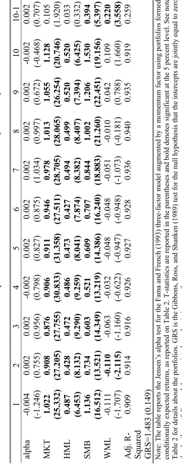
Table 5 presents the Jensen’s alpha test for a four-factor model, in which we add a momentum factor (WML) to the Fama and French three-factor model. Carhart (1997) and Pastor and Stambaugh (2003), among others, have also used this four-factor model to control for

systematic risks. The four-factor model is quite successful: Intercepts for all portfolios, including the trading strategy of buying expected winners and selling expected losers, are very small and statistically insignificant. Moreover, the GRS test does not reject the four-factor model at the 10 percent significance level. Interestingly, consistent with the ICAPM interpretation, loadings on risk factors usually increase from deciles of low expected returns to deciles of high expected returns. For example, all factors make positive contributions to the difference between the tenth and first deciles (column 10-1) and the contribution is significant for the momentum profit (WML) and the size premium (SMB) and marginally significant for stock market returns (MKT).

E. Robustness

In Table 6, we investigate whether our results are sensitive to microstructure issues addressed by Cooper et al. (2003), among others. In particular, we drop stocks that have prices less than one dollar at the end of the formation period and skip one quarter between formation and holding periods. The second specification also reflects the fact that the macrovariables used to construct the consumption-wealth ratio are available with a one-month delay. Table 6 shows

that our results are essentially unchanged after we take into account these microstructure concerns.

In Table 7, we use a rolling sample of ten-year observations instead of the expanding sample. Again, we find that the portfolio returns increase monotonically from the first decile (with the lowest expected returns) to the tenth decile (with the highest expected returns). Also, the decile portfolios provide a serious challenge to the CAPM: Jensen’s alfa is significant in 7 of 11 cases and the GRS test rejects the null hypothesis that the intercepts are jointly insignificant at the 5 percent level. The trading profit of buying expected winners and selling expected losers remains significantly positive after we control for Fama and French’s three factors, while it becomes insignificant for Carhart’s (1997) four-factor model. However, the GRS test indicates that the Fama and French three-factor model explains the cross section of stock returns better than the Carhart four-factor model does.

In Table 8, we use the idiosyncratic volatility constructed by Guo and Savickas (2003) instead of the consumption-wealth ratio to forecast individual stock returns. Again, the results are very similar to those reported in the preceding subsections, in which we use the consumption-wealth ratio as a forecasting variable. This result is particularly interestingly because as

mentioned above, unlike the consumption-wealth ratio, the idiosyncratic volatility is reliably available in real time.

F. Momentum and Cross-Sectional Variations of Conditionally Expected Returns

CS show that the momentum profit vanishes if we control for the expected component of past returns and thus argue that the momentum profit is explained by the cross-sectional

Cooper et al. (2003) show that their results are sensitive to microstructure concerns, e.g., excluding the stocks that have prices less than one dollar at the end of the formation period and/or skipping one month between formation and holding periods. Also, Chen (2002) and Griffins et al. (2003) find that the forecasting variables used by CS do not explain the momentum profit in multi-factor models. One possible explanation for the conflicting results is that, as pointed out by Bossaerts and Hillion (1999), Ang and Bekaert (2003), and Goyal and Welch (2003), among others, the forecasting variables used by CS have poor out-of-sample predictive power for stock returns. To investigate this issue, we try to replicate the results in CS using the forecasting variables adopted in this paper. This investigation is interesting also because, in contrast with Chen (2002), Guo (2002) shows that our macrovariables help explain the momentum profit in a variant of Campbell’s (1993) ICAPM.

In particular, we perform two independent sorts into quintiles by (1) returns in past two quarters and (2) one-quarter-ahead forecast. It should be noted that our approach differs from that in CS in two dimensions. First, we use a one-quarter-ahead forecast as a proxy for conditionally expected returns, while CS use the conditionally expected component of past returns. Our specification, which is also advocated by Cooper et al. (2003), is appropriate because it is directly motivated from recent theoretical works, e.g., Berk et al. (1999) and

Johnson (2002), among others. Second, we use independent sorts rather than the sequential sorts in CS, e.g., first by expected returns and then by raw returns. However, we find qualitatively the same results using the sequential sorts.

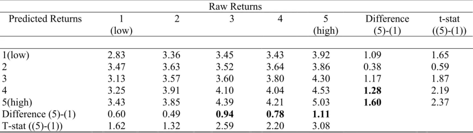
Table 9 reports returns on the 25 portfolios, which are the intersections of two

independent sorts on past returns and expected returns. Portfolios sorted on past returns are in columns, ranging from the portfolio of stocks with the lowest past returns (column 1) to portfolio

of stocks with the highest past returns (column 5). Portfolios sorted on expected returns are in rows, ranging from the portfolio of stocks with the lowest expected returns (row 1) to the portfolio of stocks with the highest expected returns (row 5). Therefore, portfolios in the same column have similar past returns and portfolios in the same row have similar expected returns. We find that, after we control for past returns, the average return on the portfolio of stocks with the highest expected returns (row 5) is significantly higher than the average return on the portfolio of stocks with the lowest expected returns (row 1) in columns 3, 4, and 5. Similarly, after we control for expected returns, the average return on the portfolio of stocks with the highest past returns (column 5) is significantly higher than the average return on the portfolio of stocks with the lowest past returns (column 1) in rows 4 and 5. Therefore, consistent with the results in Table 5, the portfolios sorted on expected return are related to the portfolios sorted on past returns. However, in contrast with CS, Table 9 shows that the momentum is not completely

explained by the cross-sectional variations in expected returns and vice versa.16

Of course, this result does not imply that our forecasting variables are not related to the momentum profit: Table 10 shows that the consumption-wealth ratio and realized stock market volatility are strong predictors of the momentum profit reported in Table 1.17 Rather, it reflects the fact that, as shown in Table 5, the momentum is only one of the priced risk factors and thus does not fully explain the cross-sectional variations in conditionally expected returns, which also reflect loadings on the other risk factors in an ICAPM. In other words, although the exercise in Table 9 provides an interesting link between the momentum and the conditionally expected stock returns, it is not a formal test of such relation and thus should be interpreted with caution.

16 _{We confirm the results by Cooper et al. (2003) that the momentum profit becomes more significant in the double}

sorts if we (1) exclude the stocks that have prices less than one dollar at the end of the formation period and/or (2) skip one quarter between the formation and holding periods.

G. Portfolio Performance over Long Horizons

Jegadeesh and Titman (2001) show that returns on the momentum strategy turn negative if we increase the holding periods. We find a similar pattern using the momentum profit

constructed from quarterly return data. As shown in Figure 4, the momentum profit initially rises and then falls with the holding periods and it turns negative after 14 quarters. While Jegadeesh and Titman (2001) suggest that this result is consistent with behavioral models of Daniel et al. (1998) and Hong and Stein (1999), it is also consistent with the cross-sectional variations in conditionally expected returns if expected returns follow a mean-reverting process. For example, after a positive (negative) shock to its expected return, a stock initially has above (below)

average returns but reverts to the average in the long run. Figure 5 shows that the momentum profit sorted on expected returns first rises and then falls with holding periods: It is significantly positive only for the first 5 quarters.

IV.

Conclusion

There is a large amount of evidence that the CAPM does not explain the cross section of stock returns. However, the CAPM is alive and well because the failure of the CAPM reflects two things: (1) irrational pricing or data snooping and (2) ICAPM, and financial economists disagree on which explanation is closer to reality. In this paper, we provide some new insights on this controversy by forming portfolios on conditionally expected returns, which is motivated from ICAPM and thus not vulnerable to the criticisms of irrational pricing and data snooping. We find support for the intertemporal pricing because the CAPM fails to explain returns on these portfolios.

In contrast with recent work by Chordia and Shivakumar (2002), the momentum profit remains significant after we control for conditionally expected returns. This is because the momentum profit is only one of the risk factors and the cross section of conditionally expected returns also reflects the dispersion of loadings on other risk factors.

We also find that returns on the decile portfolios sorted on expected returns are significantly correlated with the size and value premiums as well as the momentum profit. In particular, they appear to be explained by Carhart’s (1997) four-factor model. These results suggest that the CAPM anomalies cannot be attributed entirely to data snooping and irrational pricing. However, it is important to note that our results do not lead to the conclusion that the CAPM anomalies are fully explained by rational pricing or that Carhart’s four-factor model is the replacement for the CAPM. These issues can be properly addressed only in the context of a fully fledged ICAPM, and Brennan et al. (2003) and Campbell and Vuolteenaho (2003), among others, have provided some tentative and interesting results. We believe that further investigation along these lines show promise for uncovering the risk-return tradeoff in the stock market.

Reference:

Ang, A., and G. Bekaert, 2003, Stock Return Predictability: Is it There?, Working Paper, Columbia Business School.

Ang, A., and J. Chen, 2003, CAPM over the Long Run: 1926-2001, Working Paper, Columbia Business School.

Banz, R., 1981, The Relationship Between Return and Market Value of Common Stocks, Journal of Financial Economics, 9, 3-18.

Basu, S., 1977, Investment Performance of Common Stocks in Relation to Their Price— Earnings Ratios: A Test of the Efficient Market Hypothesis, Journal of Finance, 32, 663-82. Berk, J., 1995, A Critique of Size Related Anomalies, Review of Financial Studies, 8, 275-286. ________, R. Green, and V. Naik, 1999, Optimal Investment, Growth Options, and Security Returns, Journal of Finance, 54, 1553-1608.

Bernanke, B., and M. Gertler, 1989, Agency Costs, Net Worth, and Business Fluctuations, American Economic Review, 79, 14-31.

Bossaerts, P., and P. Hillion, 1999, Implementing Statistical Criteria to Select Return Forecasting Models: What Do We Learn?, Review of Financial Studies, 12, 405-428.

Brennan, M., A. Wang, and Y. Xia, 2003, Estimation and Test of a Simple Model of Intertemporal Asset Pricing, Journal of Finance, forthcoming.

Campbell, J., 1987, Stock Returns and the Term Structure, Journal of Financial Economics, 18, 373-399.

________, 1993, Intertemporal Asset Pricing without Consumption Data, American Economic Review, 83, 487-512.

________, and J. Cochrane, 1999, By Force of Habit: A Consumption-Based Explanation of Aggregate Stock Market Behavior, Journal of Political Economy, 107, 205-251.

________, M. Lettau, B. Malkiel, and Y. Xu, 2001, Have Individual Stocks Become More Volatile? An Empirical Exploration of Idiosyncratic Risk, Journal of Finance, February 2001, 56 (1), 1-43.

________, and T. Vuolteenaho, 2003, Bad Beta, Good Beta, Unpublished working paper, Harvard University.

Carhart, M., 1997, On Persistence in Mutual Fund Performance, Journal of Finance, 52, 57-82. Chen, J., 2002, Intertemporal CAPM and the Cross-Section of Stock Returns, Unpublished working paper, University of Southern California.

Chordia, T., and L. Shivakumar, 2002, Momentum, Business Cycle, and Time-Varying Expected Returns, Journal of Finance, 57, 985-1019.

Cooper, M., R. Gutierrez, and A. Hameed, 2003, Market States and Momentum, Journal of Finance, Forthcoming.

Dai, Q., 2003, Time-Series and Cross-Sectional Variation of Expected Returns, Unpublished working paper, Stern School of Business.

Daniel, K., D. Hirshleifer, and A. Subrahmanyam, 1998, Investor Psychology and Security Market Under- and Over-Reactions, Journal of Finance, 53, 1839-1885.

Fama, E., 1991, Efficient Capital Markets: II, Journal of Finance, 46, 1575-1617.

Fama, E., and K. French, 1993, Common Risk Factors in the Returns on Stocks and Bonds, Journal of Financial Economics, 33, 3-56.

________, 1996, Multifactor Explanations of Asset Pricing Anomalies, Journal of Finance, 51, 55-84.

________, 2003, The CAPM: Theory and Evidence, Working Paper No. 550, Center for Research in Security Prices, University of Chicago.

Fama, E. and J. MacBeth, 1973, Risk, Return and Equilibrium: Empirical Tests, Journal of Political Economy, 81, 607-636.

Ferson, W. and C. Harvey, 1999, Conditioning Variables and the Cross-section of Stock Returns, Journal of Finance, 54, 1325-60.

Gibbons, M., S. Ross, and J. Shaken, 1989, A Test of the Efficiency of a Given Portfolio, Econometrica, 57, 1121-1152.

Gomes, J., L, Kogan, and L. Zhang, 2003, Equilibrium Cross Section of Returns, Journal of Political Economy, 111, 693-732.

Goyal, A. and P. Santa-Clara, 2003, Idiosyncratic Risk Matters!, Journal of Finance, Vol. 58, pp. 975-1007.

Goyal, A., and I. Welch, 2003, Predicting the Equity Premium with Dividend Ratios, Management Science, 49, 639-654.

Graham, B. and D. Dodd, 1934, Security Analysis, First Edition, McGraw Hill, New York. Griffin, J., S. Ji, and S. Martin, 2003, Momentum Investing and Business Cycle Risk: Evidence from Pole to Pole, Journal of Finance, Forthcoming.

Guo, H., 2002, Time-Varying Risk Premia and The Cross Section of Stock Returns, working paper, 2002-013B, Federal Reserve Bank of St. Louis.

________, 2003a, On the Out-of-Sample Predictability of Stock Market Returns, Forthcoming, Journal of Business.

________, 2003b, Limited Stock Market Participation and Asset Prices in a Dynamic Economy, Forthcoming, Journal of Financial and Quantitative Analysis.

______, and R. Savickas, 2003, Idiosyncratic Volatility, Stock Market Volatility, and Expected Stock Returns, working paper 2003-028A, Federal Reverse Bank of St. Louis.

Harvey, C., 1989, Time-Varying Conditional Covariances in Tests of Asset Pricing Models, Journal of Financial Economics, 24, 289-317.

Hong, H., and J. Stein, 1999, A Unified Theory of Underreaction, Momentum Trading and Overreaction in Asset Markets, Journal of Finance, 54, 2143-2184.

Jagannathan, R. and Z. Wang, 1996, The Conditional CAPM and the Cross-Section of Expected Returns, Journal of Finance, 51, 3-53.

Jegadeesh, N., and S. Titman, 1993, Returns to Buying Winners and Selling Losers: Implications for Stock Market Efficiency, Journal of Finance, 48, 65-91.

________, 2001, Profitability of Momentum Strategies: An Evaluation of Alternative Explanations, Journal of Finance, 56, 699-720.

Johnson, T., 2002, Rational Momentum Effects, Journal of Finance, 57, 585-608.

Lakonishok, J., A. Shleifer, and R. Vishny, 1994, Contrarian Investment, Extrapolation, and Risk, Journal of Finance, 49, 1541-78.

Lettau, M. and S. Ludvigson, 2001a, Consumption, Aggregate Wealth, and Expected Stock Returns, Journal of Finance, 56, 815-49.

________, 2001b, Resurrecting the (C)CAPM: A Cross-Sectional Test when Risk Premia are Time-Varying, Journal of Political Economy, 109, 1238-1287.

________, 2003, Measuring and Modeling Variation in the Risk-Return Tradeoff, Unpublished working paper, New York University.

Lewellen, J. and S. Nagel, 2003, The Conditional CAPM Does not Explain Asset-Pricing Anomalies, NBER working paper No. 9974.

Lintner, J., 1965, Security Prices, Risk and Maximal Gains from Diversification, Journal of Finance, 20, 587-615.

MacKinlay, A., 1995, Multifactor Models Do Not Explain Deviations from the CAPM, Journal of Financial Economics, 38, 3-28.

Merton, R., 1973, An Intertemporal Capital Asset Pricing Model, Econometrica, 41, 867-887. ______, 1980, On Estimating the Expected Return on the Market: An Exploratory Investigation, Journal of Financial Economics, 8, 323-361.

Pastor, L., and R. Stambaugh, 2003, Liquidity Risk and Expected Stock Returns, Journal of Political Economy, 111, 642-85.

Patelis, A., 1997, Stock Return Predictability and The Role of Monetary Policy, Journal of Finance, 1951-72.

Petkova, R., and Zhang, L., 2003, Is Value Riskier Than Growth? Unpublished working paper, University of Rochester.

Schwert, G., 1990, Indexes of Stock Prices from 1802 to 1987, Journal of Business, 63, 399-426. Sharpe, W., 1964, Capital Asset Prices: A Theory of Market Equilibrium Under Conditions of Risk, Journal of Finance, 19, 425-42.

Whitelaw, R., 1994, Time Variations and Covariations in the Expectation and Volatility of Stock Market Returns, Journal of Finance, 49, 515-541.

Figure 1. Momentum Based on Past Quarterly Returns (Dashed Line) and Past Monthly Returns (Solid Line)

Figure 2. Cross-Sectional Average of Adjusted R-Squared -1 -0.5 0 0.5 54-Q3 59-Q3 64-Q3 69-Q3 74-Q3 79-Q3 84-Q3 89-Q3 94-Q3 99-Q3 0 0.1 0.2 54-Q3 59-Q3 64-Q3 69-Q3 74-Q3 79-Q3 84-Q3 89-Q3 94-Q3 99-Q3

Figure 3. Momentum Sorted on Expected Returns (Solid Line) and Past Returns (Dashed Line)

Figure 4. Momentum Profit Based on Past Returns: Various Holding Periods -0.02 0 0.02 0.04 1 4 7 10 13 16 19 -0.8 -0.4 0 0.4 54-Q3 59-Q3 64-Q3 69-Q3 74-Q3 79-Q3 84-Q3 89-Q3 94-Q3 99-Q3

Figure 5. Momentum Profit Based on Expected Returns: Various Holding Periods -0.01 0 0.01 0.02 1 4 7 10 13 16 19

Table 1. Returns on Portfolios Sorted on Past Returns 1 2 3 4 5 6 7 8 9 10 10-1 1954:Q3-2002:Q4 0.025 0033 0.035 0.035 0.037 0.037 0.038 0.038 0.042 0.047 0.023 (2.858) 1954:Q3-1978:Q4 0.029 0.033 0.035 0.034 0.036 0.036 0.037 0.038 0.042 0.046 0.017 (1.588) 1979:Q1-2002:Q4 0.020 0.032 0.036 0.036 0.039 0.039 0.039 0.038 0.041 0.048 0.029 (2.429)

Note: The table reports summary statistics of returns on portfolios formed on past returns. At the end of each quarter

t, we sort stocks equally into ten portfolios on returns in the past two quarters, ranging from the portfolio of stocks with the lowest past returns (first decile) to the portfolio of stocks with the highest past returns (tenth decile). These portfolios are held over the next two quarters. The last column is the momentum profit of buying past winners (column 10) and selling past losers (column 1).

Table 2. Returns on Portfolios Sorted on Conditionally Expected Returns 1 2 3 4 5 6 7 8 9 10 10-1 1954:Q3-2002:Q4 0.033 0.034 0.035 0.036 0.036 0.037 0.039 0.041 0.043 0.044 0.012 (3.297) 1954:Q3-1978:Q4 0.034 0.034 0.034 0.034 0.035 0.035 0.037 0.041 0.043 0.047 0.012 (2.341) 1979:Q1-2002:Q4 0.031 0.034 0.037 0.038 0.038 0.040 0.040 0.041 0.044 0.042 0.011 (2.336)

Note: The table reports summary statistics of returns on portfolios formed on conditionally expected returns. At the end of each quarter t, we make a one-quarter-ahead forecast for returns on each stock using the consumption-wealth ratio, realized stock market variance, the stochastically detrended risk-free rate, and past stock market returns as predictive variables. We require at least two years of observations and use an expanding sample. We then sort stocks equally into ten portfolios on this forecast, ranging from the portfolio of stocks with the lowest expected returns (first decile) to the portfolio of stocks with the highest expected returns (tenth decile). These portfolios are held over the next two quarters. The last column is the momentum profit of buying past winners (column 10) and selling past losers (column 1).

34

Table 3. Jensen’s alpha Test for CAPM: 1954:Q3 – 2002:Q4

123456789 10 10 -1 alpha -0.000 _(-0.084) 0.005 _(1.230) 0.007 _(2.137) 0.008 _(2.535) 0.007 _(2.260) 0.007 _(2.113) 0.008 _(2.007) 0.009 _(2.112) 0.101 _(2.042) 0.084 _(1.374) 0.009 _(2.652) MKT 1.221 (14.749) 1.010 (15.319) 0.923 _(14.906) 0.922 _(16.303) 0.968 _(15.943) 1.020 (15.575) 1.085 (15.918) 1.157 (15.975) 1.243 (15.052) 1.397 _(13.911) 0.176 _(3.383) Adj. R- Squared 0.654 0.712 0.724 0.757 0.745 0.737 0.719 0.706 0.676 0.635 0.087 GRS=2.931 (0.002) he ta ble re po rts t he Jen se n’s alp ha test fo r the C A PM u

sing portfolios form

ed on conditiona lly expecte d ret urns, as repo rted i n Table 2. T-statistics are orte d in the pa rent heses a nd b old de notes significant at t he 5

percent level. See

note of Table 2 for details

about the port folios. GRS is t he Gibb on s, Ross, and nke n ( 19 89 ) test fo r th e null h ypothesis t

hat the interc

epts are jo in tly equal to zero fo r the decile

portfolios and the ass

ociated p-value is i n pa re ntheses.

35

Table 4. Jensen’s alpha Test for the Fam

a

and French Three-Factor Model: 1954:Q3 – 2002:Q4

123456789 10 10 -1 alpha -0.007 _(-2.521) -0.002 _(-0.755) 0.000 _(0.033) 0.001 _(0.269) 0.000 _(0.125) 0.000 _(0.223) 0.001 _(0.340) 0.002 _(1.020) 0.003 _(1.289) 0.002 _(0.736) 0.010 _(3.062) MKT 1.037 (24.539) 0.922 (26.750) 0.885 _(27.126) 0.910 _(30.053) 0.918 _(31.037) 0.952 (27.081) 0.985 (28.151) 1.014 (27.419) 1.050 (25.539) 1.113 _(19.332) 0.076 _(1.232) HML 0.520 _(6.330) 0.460 _(7.575) 0.490 _(8.506) 0.496 _(8.296) 0.487 _(7.327) 0.487 _(7.246) 0.509 _(7.834) 0.501 _(8.038) 0.508 _(7.100) 0.488 _(5.808) -0.031 _(-0.293) SMB 1.169 (16.643) 0.767 (13.322) 0.622 _(13.979) 0.531 _(14.183) 0.623 _(15.027) 0.722 (16.000) 0.860 (18.727) 1.005 (20.660) 1.193 (21.681) 1.497 _(18.130) 0.328 _(4.115) Adj. R- Squared 0.906 0.910 0.914 0.926 0.927 0.928 0.935 0.940 0.935 0.917 0.186 GRS=1.895 (0.048) Note: T he ta ble re po rts t he Jen se n’s alp ha test fo r the Fam a and Fr en ch ( 199 3) thr ee-fa ctor m od el u sing po rt fo lio s fo rm ed on co nditionally expected returns, as

reported in Table 2. T-statistic

s are r ep orte d in the pa rent heses a nd bo ld de not es significant at t he 5

percent level. See note

of Table 2 f or de tails about t he po rt fo lio s. GRS is th e Gib bon s, R oss, an d Sh ank en (198 9) test

for the null hy

pot

hesis that the i

ntercepts are jointly equal to

zero

for t

he

decile portfolios and the

associated p-val ue is i n pare ntheses.

36

Table 5. Jensen’s alpha Test for

the Four-Factor M odel: 1954:Q3 – 2002:Q4 123456789 10 10 -1 alpha -0.004 _(-1.246) 0.002 _(0.755) 0.002 _(0.956) -0.002 _(0.798) 0.002 _(0.827) 0.002 _(0.875) 0.002 _(1.034) 0.002 _(0.997) 0.002 _(0.672) -0.002 _(-0.468) 0.002 _(0.707) MKT 1.022 (25.332) 0.908 (27.205) 0.876 _(27.755) 0.906 _(30.833) 0.911 _(31.358) 0.946 (27.511) 0.978 (28.705) 1.013 (28.065) 1.055 (26.254) 1.128 _(20.746) 0.105 _(1.920) HML 0.487 _(6.453) 0.428 _(8.132) 0.472 _(9.290) 0.486 _(9.259) 0.473 _(8.041) 0.427 _(7.874) 0.494 _(8.382) 0.499 _(8.407) 0.520 _(7.394) 0.520 _(6.425) 0.033 _(0.332) SMB 1.136 (16.512) 0.734 (13.521) 0.603 _(14.349) 0.521 _(13.219) 0.609 _(14.386) 0.707 (16.240) 0.844 (18.883) 1.002 (21.260) 1.206 (22.451) 1.530 _(19.156) 0.394 _(5.397) WML -0.111 _(-1.707) -0.110 _(-2.115) -0.063 _(-1.160) -0.032 _(-0.622) -0.048 _(-0.947) -0.048 _(-0.948) -0.051 _(-1.073) -0.010 _(-0.181) 0.042 _(0.788) 0.109 _(1.660) 0.220 _(3.558) Adj. R- Squared 0.909 0.914 0.916 0.926 0.927 0.928 0.936 0.940 0.935 0.919 0.259 GRS=1.483 (0.149) he ta ble re po rts t he Jen se n’s alp ha test fo r the Fam a and Fre nc h (1 99 3) th ree -facto r m odel a ugm ented by a m om entu m facto r u sin g po rt fo lio s fo rm ed on ditionally ex pecte d retur ns, as re po rted o n Ta ble 2. T-statis tics are re ported i n t he pare nthe se s a nd bold de notes significa nt at the 5 percent level. See note of 2 f or details ab out t he po rtf olios. GR S is th e Gib bon s, Ro ss, an d Sh an ken ( 198 9) test for th e nu ll h yp ot he sis th at th e in tercepts are j ointly equal t o zero for portfolios and t he associ ated p -value is in pare ntheses.

Table 6. Portfolios Sorted on Conditionally Expected Returns with Control for Microstructure

1 2 3 4 5 6 7 8 9 10 10-1

Mean

0.032 0.035 0.034 0.035 0.035 0.036 0.037 0.039 0.041 0.043 0.011

(3.170)

alfa from the CAPM 0.000

(0.013) (1.709)0.006 (2.096)0.007 (2.503)0.008 (2.257)0.007 (2.006)0.007 (1.796)0.007 (1.821)0.008 (1.611)0.008 (1.280)0.008 (2.465)0.007

GRS=3.244(0.001)

alfa from the Fama and French Three-Factor model

-0.007 (-2.325) -0.000 (-.113) -0.000 (-.099) 0.001 (0.269) 0.000 (0.129) 0.000 (0.062) -0.000 (-.023) 0.001 (0.531) 0.001 (0.588) 0.001 (0.558) 0.008 (2.898) GRS=2.328(0.013)

alfa from the Four-Factor Model -0.003 (-.849) 0.003 (1.314) 0.002 (0.737) 0.00 (0.851) 0.001 (0.339) 0.001 (0.550) 0.001 (0.635) 0.002 (0.654) 0.000 (0.149) -0.001 (-.327) 0.002 (0.526) GRS=1.480(0.150)

Note: The table reports summary statistics of returns on portfolios formed on conditionally expected returns. The specifications are the same as these in Table 2 except that (1) we exclude stocks with a price less than $1 at the end of the formation period and (2) skip a quarter between formation and holding periods. See notes of Tables 2-5 for other information.

Table 7. Portfolios Sorted on Conditionally Expected Returns with Rolling Samples

1 2 3 4 5 6 7 8 9 10 10-1

Mean

0.033 0.035 0.036 0.036 0.036 0.037 0.038 0.041 0.043 0.044 0.010

(2.824)

alfa from the CAPM 0.000

(0.031) (1.317)0.005 (2.077)0.007 (2.198)0.007 (2.355)0.008 (2.181)0.008 (2.075)0.008 (2.130)0.009 (1.887)0.009 (1.300)0.008 (2.196)0.008

GRS=2.399 (0.011)

alfa from the Fama and French Three-Factor model

-0.007 (-2.242) -0.001 (-.488) -0.000 (-.019) -0.000 (-.089) 0.001 (0.286) 0.000 (0.200) 0.001 (0.312) 0.002 (0.931) 0.003 (1.289) 0.002 (0.532) 0.008 (2.470) GRS=1.549 (0.125)

alfa from the Four-Factor Model -0.003 (-1.059) 0.003 (1.308) 0.003 (1.374) 0.002 (0.748) 0.002 (0.894) 0.001 (0.495) 0.001 (0.503) 0.002 (0.842) 0.002 (0.654) -0.002 (-.667) 0.001 (0.284) GRS=1.981 (0.038)

Note: The table reports summary statistics of returns on portfolios formed on conditionally expected returns. The specifications are the same as these in Table 2 except that we use a rolling sample of 10 years. See notes of Tables 2-5 for other information.

Table 8. Portfolios Sorted on Conditionally Expected Returns Using Idiosyncratic Volatility

1 2 3 4 5 6 7 8 9 10 10-1

Mean

0.032 0.036 0.036 0.037 0.036 0.036 0.038 0.040 0.042 0.042 0.011

(2.613)

alfa from the CAPM -0.001 (-.116) 0.006 (0.997) 0.007 (1.388) 0.009 (1.963) 0.009 (1.982) 0.009 (2.130) 0.010 (2.479) 0.012 (2.766) 0.013 (2.416) 0.011 (1.560) 0.012 (2.800) GRS=3.147 (0.001)

alfa from the Fama and French Three-Factor model

-0.011 (-2.770) -0.004 (-1.289) -0.002 (-.608) 0.000 (0.132) -0.000 (-.018) 0.000 (0.135) 0.002 (0.749) 0.004 (1.572) 0.005 (1.710) 0.003 (0.899) 0.014 (3.321) GRS=2.005 (0.037)

alfa from the Four-Factor Model -0.006 (-1.315) -0.001 (-.365) -0.001 (-.197) 0.001 (0.469) 0.000 (0.173) 0.001 (0.537) 0.003 (1.183) 0.004 (1.571) 0.004 (1.366) 0.002 (0.412) 0.008 (1.832) GRS=1.074 (0.387)

Note: The table reports summary statistics of returns on portfolios formed on conditionally expected returns. The specifications are the same as these in Table 2 except that we use the idiosyncratic volatility constructed by Guo and Savickas (2003) instead of the consumption-wealth ratio in the forecasting equation. The sample spans from 1965:Q4 to 2002:Q4. See notes of Tables 2-5 for other information.

Table 9. Returns on Portfolios Ranked by Raw Returns and Predicted Returns Raw Returns Predicted Returns 1 (low) 2 3 4 5 (high) Difference (5)-(1) t-stat ((5)-(1)) 1(low) 2.83 3.36 3.45 3.43 3.92 1.09 1.65 2 3.47 3.63 3.52 3.64 3.86 0.38 0.59 3 3.13 3.57 3.60 3.80 4.30 1.17 1.87 4 3.25 3.91 4.10 4.04 4.53 1.28 2.19 5(high) 3.43 3.85 4.39 4.21 5.03 1.60 2.37 Difference (5)-(1) 0.60 0.49 0.94 0.78 1.11 T-stat ((5)-(1)) 1.62 1.32 2.59 2.20 3.08

Note: The table reports returns on the 25 portfolios, which are the intersections of the two independent sorts on past returns and expected returns. Portfolios sorted on past returns are in columns, ranging from the portfolio of stocks with the lowest past returns (column 1) to the portfolio of stocks with the highest past returns (column 5). Portfolios sorted on expected returns are in rows, ranging from the portfolio of stocks with the lowest expected returns (row 1) to the portfolio of stocks with the highest expected returns (row 5). Bold denotes that the difference between returns on two portfolios is significant at the 5 percent level.

Table 10. Forecasting One-Quarter-Ahead Momentum Sorted on Raw Returns Intercept r_{m t,−1} cay_{t−1 σm t}2_{,−1 rrel}

t−1 D1 R2 Panel A. 1952:Q3 – 2002:Q4 1 1.141 (2.965) -0.026 (-0.214) -1.914 (-2.837) -9.326 (-3.543) 0.034 (0.015) 0.096 2 1.159 (2.817) (-2.686)-1.948 (-4.205)-9.144 0.105 3 1.035 (3.016) 0.092 (0.848) (-2.835)-1.698 -7.245 (-3.222) 1.081 (0.473) (-4.977)-0.107 0.267 Panel B. 1952:Q3 – 1977:Q4 4 0.620 (1.422) -0.151 (-0.773) -0.971 (-1.247) -17.443 (-3.187) 6.547 (1.275) 0.225 5 1.181 (3.423) (-3.268)-1.984 (-3.048)-15.424 0.211 6 0.655 (1.642) 0.043 (0.238) -1.015 (-1.423) -13.997 (-2.934) 9.128 (2.178) -0.103 (-4.097) 0.390 Panel C. 1978:Q1 – 2002:Q4 7 1.523 (2.162) (-0.015)-0.002 (-2.091)-2.556 (-2.928)-9.507 (-0.440)-1.062 0.065 8 1.525 (2.159) -2.560 (-2.073) -9.399 (-3.697) 0.083 9 1.231 (1.982) 0.070 (0.531) -2.016 (-1.882) -7.328 (-2.732) -0.879 (-0.390) -0.106 (-3.215) 0.220 Note: The table reports the regression results of the momentum profit (last column of Table 1) on predetermined variables. r_{m t,−1} is lagged stock market return; cay_t−1 is the consumption-wealth ratio; σ2_{m t,−1} is realized stock market variance; rrel_t−1 is the stochastically detrended risk-free rate; and D1 is a dummy variable that is equal to 1 for the first quarter and zero otherwise. Bold denotes significant at the 5 percent level.