1
Instability
wave-streak
interactions
in
a
supersonic
boundary
layer
Pedro
Paredes
†
,
Meelan
M.
Choudhari,
and
Fei
Li
ComputationalAeroSciencesBranch,NASALangleyResearchCenter,Hampton,VA23681, USA
Optimal initial conditions fortransient growth in a two-dimensional boundary layer flow correspond to stationary, counter-rotating vortices that subsequentlydevelop into streamwise elongated streaks,whichare characterizedby analternating pattern oflow and high streamwise velocity. For incompressible flows, previous studies have shown that boundary layer modulation due to streaks below a threshold amplitude level can stabilize the Tollmien-Schlichtinginstabilitywaves, resultingin a delay in theonset of laminar-turbulenttransition.Inthesupersonicregime,thelinearly,most-amplifiedwaves becomethree-dimensional,correspondingtooblique,first-modewaves.Thischangeinthe characterofdominantinstabilitiesleadstoanimportantchangeinthetransitionprocess, whichisnow dominatedbyoblique breakdownvianonlinearinteractionsbetweenpairs offirst-modewavesthat propagateatequal butoppositeangleswithrespecttothefree stream.Becausetheobliquebreakdownprocessischaracterizedbyarapidamplification of stationary streamwise streaks, artificial excitation of such streaks may be expected to promote transition in a supersonic boundary layer. Indeed, suppression of those streaks has been shown to delay the onset of transition in prior literature. Consistent with thosefindings, thepresent study showsthat optimally growingstationary streaks indeed destabilize thefirst-mode waves,but onlywhen the spanwisewavelength of the instability waves is equal to or smaller than twice the streak spacing. Transition in a benign disturbance environment typically involves first-mode waves with significantly longer spanwise wavelengths, and hence, these waves are stabilized by the optimal growth streaks. Thus, as long as the amplification factors for the destabilized, short wavelengthinstabilitywavesremainbelowthethresholdlevelfortransition,asignificant netstabilizationisachieved,yieldingatransitiondelaythatiscomparabletothelength ofthelaminarregionin theuncontrolledcase.
Key words:boundarylayertransition,supersonicflow,passiveflowcontrol
1. Introduction
Laminar flow technology is recognized as a potential breakthrough for economically viable and environmentally friendly supersonic aircraft. Benefits of extended laminar flow include: reduced skin friction drag, i.e., lower fuel burn, increased range, reduced aircraft weight, and reduced emissions and ozone impact, especially in the high altitude regime of supersonic flight. Additionally, the lower weight implies both a weaker sonic boom signature at the ground level and reduced acoustic emissions during take-off and landing.
2 P. Paredes, M. M. Choudhari, and F. Li
Reduced skin friction of the laminar flow also translates into reduced aerodynamic heating of wing and empennage surfaces. Therefore, the prediction and control of transition onset in high-speed flows is a key issue for optimizing the performance of next-generation supersonic vehicles.
At low levels of background disturbances, transition is initiated by the exponential amplification of linearly unstable eigenmodes, i.e., modal instabilities of the laminar boundary layer. In two-dimensional boundary layers, different instability mechanisms dominate the exponential growth phase depending on the flight speed. Planar, i.e., two-dimensional, Tollmien-Schlichting (TS) waves are the most unstable in the incompressible regime, whereas oblique first-mode instabilities correspond to the most amplified distur-bances in supersonic boundary layers. The hypersonic regime is again dominated by the growth of planar acoustic waves of the second mode, i.e., Mack mode type (Mack 1984). Focusing on the supersonic regime, Fasel et al. (1993) conducted a direct numerical simulation of the early transition stages for a Mach 1.6 boundary layer and showed that a pair of oblique modes with equal but opposite wave angle interact nonlinearly and lead to transition. Subsequently, this oblique breakdown mechanism was studied by means of the nonlinear form of the Parazolized Stability Equations (PSE) by Chang & Malik (1994) and high Reynolds number asymptotic theory by Leib & Lee (1995). Chang & Malik (1994) confirmed that the primary breakdown mechanism in supersonic boundary layers constitutes a wave-vortex triad formed by the two oblique modes and a stationary streamwise vortex mode. The oblique waves are linearly amplified until nonlinear saturation sets in, while the vortex mode with half wavelength of the oblique waves results from the nonlinear interactions. The laminar-turbulent transition onset begins when higher harmonics are also generated by nonlinear interactions, which grow rapidly to reach amplitudes on the order of the amplitude of primary oblique waves. The theoretical analysis by Leib & Lee (1995) confirmed that the explosive growth of oblique instability waves is a generic feature of instability development in both insulated- and cooled-wall supersonic boundary layers. More recent numerical studies (e.g., Mayeret al.
2011b,a, 2014) have confirmed that in a supersonic boundary layer, the oblique-mode transition scenario requires lower initial amplitudes than other transition mechanisms, as fundamental or subharmonic secondary instability mechanisms initiated by the linear growth of the two-dimensional mode. Therefore, oblique breakdown is the most likely scenario for natural transition in low-disturbance environments.
In the presence of sufficiently strong external disturbances in the form of either freestream turbulence (FST) or three-dimensional wall roughness, streamwise streaks involving alternately low and high streamwise velocity have been observed to appear in incompressible boundary layers (Klebanoff 1971). Further research in the incompressible regime has shown that high amplitude streaks can become unstable to shear layer instabilities that lead to a form of “bypass transition” (Anderssonet al.2001). When the streak amplitudes are low enough to avoid these instabilities, i.e., when the background disturbance level is moderate, the streaks can actually reduce the growth of the TS waves as documented in both experimental and theoretical studies (Boikoet al.1994; Cossu & Brandt 2002; Bagheri & Hanifi 2007). The stabilizing effect of stationary streaks in low-speed boundary layers has been used in passive flow control strategies to demonstrate delayed onset of transition by using micro vortex generators (MVGs) along the body surface (Franssonet al.2006; Shahinfaret al.2012).
Among the limited experimental research focusing on the tripping of high-speed boundary layer flows by using three-dimensional roughness elements is the investigation of Holloway & Sterrett (1964), who used a single row of spherical roughness elements partially recessed within a flat-plate model in the NASA Langley 20-Inch Mach 6 tunnel,
which has a conventional freestream turbulence level. Data for multiple boundary layer edge Mach numbers was obtained by varying the plate mounting angle. They found that, for cases with the smallest roughness diameters, transition was delayed for Mach numbers larger than 3.7, which approximately corresponds to the lower bound for planar second mode dominance over oblique first-mode instabilities in a flat-plate boundary layer at typical wind tunnel conditions. Therefore, their results suggest that roughness induced streaks have a stabilizing influence on Mack-mode waves, but not on oblique first-mode instabilities at supersonic boundary-layer-edge conditions. As the roughness height was further increased, the transition onset location moved upstream closer to the roughness elements. Recent work (Choudhariet al.2009; Paredeset al.2016a,c) indicates that the earlier onset of transition can be attributed to the onset of high-frequency instabilities in the streaky boundary layer.
The development of roughness-induced streaks is strongly dependent on the details of the roughness element shape, height, and spanwise or azimuthal spacing. The optimal growth theory provides a conceptually simple model that can characterize the transient algebraic growth and subsequent slow decay of boundary layer streaks due to arbitrary initial disturbances, as well as providing an upper bound on the energy amplification ratio; see Schmid (2007) for a review. The transient growth arises as a result of the non-normality of disturbance equations, and the optimal growth theory seeks to maximize the disturbance growth between a selected pair of streamwise locations. Regardless of the flow Mach number, the disturbances experiencing the highest magnitude of transient growth have been found to be stationary streaks that arise from initial perturbations that correspond to streamwise vortices. The secondary instability of optimal streaks with moderate-to-high finite initial amplitudes in supersonic and hypersonic boundary layers has been addressed in recent works by the present authors (Paredes et al. 2016a,c). They found that the mode shapes associated with secondary instabilities were similar to those found in low-speed boundary layers (Andersson et al. 2001). However, while secondary instability modes of both fundamental and subharmonic spanwise wavelengths exhibit comparable amplification factors in low-speed flows, the secondary instability with subharmonic spanwise wavelengths controls the onset of transition in supersonic flows for moderate streak amplitudes. The rather unique behavior of subharmonic mode amplifi-cation is shown to be related to the destabilizing influence of small amplitude streaks on oblique first-mode disturbances, which tend to have longer spanwise wavelengths than those of the optimal stationary disturbances. The destabilization of long wavelength first mode disturbances was also observed in the DNS computations of Choudhariet al.
(2013) behind isolated roughness elements. These computational results may explain the experimental findings of Holloway & Sterrett (1964) at supersonic boundary-layer-edge conditions, because they found an upstream movement of the transition front with any roughness height at a supersonic edge Mach number of 4.8.
The introduction of streaks in a supersonic boundary layer, in which the transition onset is driven by oblique first-mode instabilities, is expected to have a destabilizing influence and promote transition because of the following reasons: (i) the nonlinear interaction of oblique first-mode wave pairs form statoinary streamwise streaks; (ii) optimal growth streamwise streaks have been found to destabilize subharmonic first-mode waves (Paredeset al.2016c); (iii) the wake of discrete roughness elements have been experimentally observed to promote transtion by Holloway & Sterrett (1964). However, the effect of lower streak amplitudes, i.e., stable or at most weakly unstable streaks, on the growth of the entire family of oblique first-mode instabilities has not been studied previously. The present work focuses on this problem with the goal of developing a more thorough knowledge base for transition prediction in the presence of stationary
4 P. Paredes, M. M. Choudhari, and F. Li
streaks and potentially expand the range of available techniques for transition control at supersonic edge Mach numbers.
To that end, we study the effect of a periodic array of finite-amplitude streaks on the dominant instability waves in two-dimensional boundary layers at supersonic Mach numbers, i.e., the oblique first-mode waves. Similar to Paredeset al.(2016d,c), the basic state used for the present study corresponds to an adiabatic flat plate at zero angle of incidence in a supersonic freestream flow of Mach number 3 and unit Reynolds number
Re0 = 106/m. The analysis presented herein is based on boundary layer streaks resulting from the transient growth of an optimal initial perturbation excited near the leading edge. The perturbed three-dimensional boundary layer is used as basic state for the subsequent modal instability analysis by means of the plane-marching PSE.
The paper is organized as follows. Section 2 provides a summary of the plane-marching PSE theory. The results are presented in Section 3. First, the perturbed three-dimensional boundary layers composed by the two-three-dimensional boundary layer plus the finite-amplitude optimal perturbations are analyzed. Subsequently, the instability characteristics of the oblique first-mode waves for such basic states are studied, as well as the overall effect of the streaks on the transition onset location. Finally, conclusions are presented in Section 4.
2. Theory
This section introduces the methodologies used in this paper. The linear optimal growth theory based on the PSE and the application to the Mach 3 adiabatic flow plate boundary layer was presented by Paredes et al. (2016d). Following the same methodology of Paredes et al. (2016c), the linearly optimal perturbation that results in maximum energy gain at a specified downstream position is used as inflow condition for the parabolic integration of the stationary, nonlinear, plane-marching PSE (or, equiv-alently, perturbation form of the parabolic Navier-Stokes equations) to obtain a three-dimensional, spanwise-periodic, perturbed boundary layer flow. The modal instability characteristics of this perturbed flow are studied by using the linear form of the plane-marching PSE. The nonlinear evolution of moderate-to-high amplitude streaks and their instability characteristics is studied by Paredeset al.(2016c). The present paper focuses on the interaction of stable and weakly-unstable streaks with the first-mode boundary layer instability.
2.1. Plane-marching PSE
The plane-marching PSE technique extends the classical line-marching PSE for base flows with a single strongly inhomogeneous direction to base flows with a mild variation in the streamwise coordinate and strong gradients in the other two spatial directions, i.e., the wall-normal and spanwise directions in boundary layer problems. Similar to the derivation of the classical PSE, the disturbance quantities are expanded in terms of their truncated Fourier components assuming that they are periodic in time as
˜ q(x, y, z, t) = N X n=−N ˆ qn(x, y, z) exp i Z x x0 αn(x0) dx0−nωt + c.c. (2.1) The suitably nondimensionalized, Cartesian coordinate system (x, y, z) denotes stream-wise, wall-normal, and spanwise coordinates and (u, v, w) represent the corresponding velocity components. Density and temperature are denoted by ρ and T. The vector of basic state fluid variables is ¯q(x, y, z) = ( ¯ρ,u,¯ v,¯ w,¯ T¯)T, the vector of perturbation
fluid variables is ˜q(x, y, z, t) = ( ˜ρ,u,˜ v,˜ w,˜ T˜)T, and the vector of amplitude functions is
ˆ
q(ξ, η) = ( ˆρ,u,ˆ ˆv,w,ˆ Tˆ)T. The streamwise wavenumber isαandωis the angular frequency
of the perturbation.
Substituting Eq. (2.1) into the NS equations, and neglecting the viscous derivatives in
x, the plane-marching PSE can be written in a compact form as
Pn+Qn ∂ ∂y+Rn ∂2 ∂y2 +Sn ∂ ∂z+Tn ∂2 ∂z2+Vn ∂ ∂x ˆ qn(x, y, z) = Fn(x, y, z) exp −i Z x x0 αn(x0) dx0 , (2.2)
where Fn is the Fourier component of the total forcing F that contains the nonlinear
terms. The entries of the coefficient matrices forPn,Qn,Rn,Sn,Tn,Vn and vectorF
are found in Paredes (2014).
Similarly to the classical, line-marching PSE, the system of equations of the plane-marching PSE (2.2) is not fully parabolic due to the term ∂p/∂xˆ in the streamwise momentum equation (Li & Malik 1994, 1996, 1997; Haj-Hariri 1994; Andersson et al.
1998; Broadhurst & Sherwin 2008). However, for the purely stationary disturbances of interest in this work, ∂p/∂xˆ can be dropped from the equations because it is of higher order and can be neglected without any loss of accuracy. For the traveling instability waves that are also of interest in this work, the streamwise resolution is set such that
∆x >1/|α|to allow well posed parabolic integration of the PSE (Li & Malik 1997). To follow the development of finite-amplitude optimal disturbances (i.e., streaks), the nonlinear formulation of the plane-marching PSE is used (Paredes et al. 2015). For the stationary disturbances of interest in this paper, N = 0 and α0 = 0. Because of this, a single mode is integrated by using an implicit formulation to facilitate the convergence of the solution for moderate streak amplitudes (Paredes et al. 2016a,c,b, 2017). Subsequently, the linear form of the plane-marching PSE, which are recovered from Eq. (2.2) by settingF= 0, is used herein to study the linear, non-parallel stability characteristics of the modified basic state corresponding to the sum of the flat-plate boundary layer and the finite-amplitude optimal disturbance. The advantage of using the plane-marching PSE with respect to the partial-differential-equation (PDE) based two-dimensional eigenvalue problem (EVP) is that the plane-marching PSE account for the nonparallel development of the basic state. The quasiparallel assumption can lead to wavenumber and growth rate predictions with a relative error of approximately 10% when compared to plane-marching PSE or full NS results, as shown in similar problems, such as the wake behind an isolated roughness-element in a supersonic boundary layer (De Tullio et al. 2013). Nevertheless, the solution of the PDE-based EVP provides a convenient means to obtain the shape function, wavenumber, and damping/growth rate required as initial conditions for the plane-marching PSE integration.
The onset of laminar-turbulent transition is estimated using the logarithmic amplifica-tion ratio, the so-calledN-factor, based on the Mack’s energy norm E(Mack 1969) and relative to the lower bound locationxlb where the disturbance first becomes unstable,
N =− Z x xlb αi(x0)dx0+ 1/2 ln h ˆ E(x)/Eˆ(xlb) i , (2.3) where E(x) = Z z Z y ˜ qHMEq˜dydz, (2.4)
6 P. Paredes, M. M. Choudhari, and F. Li and ME= diag T¯(ξ, η) γρ¯(ξ, η)M2,ρ¯(ξ, η),ρ¯(ξ, η),ρ¯(ξ, η), ¯ ρ(ξ, η) γ(γ−1) ¯T(ξ, η)M2 . (2.5) The transition onset is assumed to occur when the peak N-factor reaches a specified value. Due to the lack of relevant experimental data, transitionN-factor thresholds are assumed to be identical for the unperturbed and perturbed boundary layer flows. The receptivity characteristics are assumed to be equivalent for both cases because the optimal perturbations are introduced with very low initial amplitude that lead to an extended linear-like behavior (as shown in the next section). Note that for the nonlinear cases, the energy measureE(x) includes the contribution of the mean-flow-distortion term.
To further understand the mechanism of instability modes, the production terms associated with the local kinetic energy transfer as a function of the streamwise location are calculated (Maliket al.1999). The streamwise rate of change of the integrated kinetic energy at a given station is given by
∂K
∂x(x) =P(x)−D(x), (2.6)
whereK is the kinetic energy of the disturbance, which is defined as
K(x) = Z z Z y ¯ ρ(˜uu˜c+ ˜vv˜c+ ˜ww˜c) dydz, (2.7) where the superscript c denotes complex conjugate,D is the viscous dissipation andP
is the production, which is given by
P(x) = Z z Z y (Iux+Iuy+Iuz+Ivx+Ivy+Ivz+Iwx+Iwy+Iwz) dydz. (2.8)
The integrand terms are called production terms and can be written as
Iux Iuy Iuz Ivx Ivy Ivz Iwx Iwy Iwz = −<(ˆuuˆc) ¯ρu¯ x −<(ˆuvˆc) ¯ρu¯y −<(ˆuwˆc) ¯ρu¯z −<(ˆvuˆc) ¯ρ¯v x −<(ˆvvˆc) ¯ρ¯vy −<(ˆvwˆc) ¯ρ¯vz −<( ˆwuˆc) ¯ρw¯ x −<( ˆwvˆc) ¯ρw¯y −<( ˆwwˆc) ¯ρw¯z . (2.9)
The sign of these terms indicates whether the local transfer of kinetic energy is stabilizing (negative) or destabilizing (positive). The viscous dissipation is not used because only the production terms are needed to judge the dominant nature of the instability mechanism associated with a given mode.
The plane-marching PSE are integrated along the streamwise coordinate by using second-order backward differentiation. A non-constant step along the streamwise direc-tion is used. For the nonlinear computadirec-tion of optimal disturbances, the streamwise grid consists of a distribution of points with constant increments of∆R= 10 in the local Reynolds number based on the similarity scale, except for streamwise positions very close to the leading edge, i.e.,R <100, where the streamwise step had to be further reduced (Paredeset al.2016c). For the modal instability analysis, the streamwise grid is coarsened to study low frequency modes to allow for the integration of the plane-marching PSE (Li & Malik 1997; Broadhurst & Sherwin 2008), although the resolution is checked for convergence in every case. Finite differences (Hermanns & Hern´andez 2008; Paredeset al.
2013) (FD-q) of sixth-order are used for discretization of the wall-normal coordinate. The wall-normal direction is discretized using from Ny = 161 to Ny = 241. The nodes are
clustered toward the wall (Paredeset al.2013). The clustering of points is dependent on the boundary layer thickness, placing half of the grid points below 10×δ, whereδis the similarity scale. The farfield boundary coordinate is set at y∞ = 150 for the nonlinear
computations, while it is set aty∞= 100×δfor the linear modal analysis. The spanwise direction is discretized with Fourier collocation points. Depending on the amplitude of the optimal growth perturbation, the number of spanwise points is varied fromNz= 16
toNz= 24 per streak wavelength, which translates into a maximum ofNz= 288 Fourier
collocation points for the most demanding case. The same spanwise grids are used to compute the evolution of both stationary and nonstationary disturbances.
No-slip, isothermal boundary conditions are used at the wall, i.e., ˆu= ˆv= ˆw= ˆT = 0. Notice that the isothermal boundary conditions may not be appropriate for all flow configurations. However, in the Mach 3 case examined in this paper, the results were insensitive to the thermal boundary condition at the surface. The amplitude functions are forced to decay at the farfield boundary by imposing the Dirichlet conditions ˆρ= ˆ
u= ˆw= ˆT = 0. The disturbance mode shapes were monitored to ensure that the chosen farfield locations were satisfactory.
The number of discretization points in all three directions was varied to ensure that the relevant flow quantities were insensitive to further improvement in grid resolution. Verification of the present plane-marching PSE module against line-marching PSE and DNS results is shown in De Tullioet al.(2013) and Paredeset al. (2015).
3. Results
Transient growth results for a zero-pressure-gradient, adiabatic wall, flat-plate bound-ary layer at freestream Mach number of M = 3 were presented by Tumin & Reshotko (2003) and Paredes et al. (2016d,c). In the present work, the nonlinear evolution of the optimal growth disturbances is investigated for moderate streaks amplitudes over an extended streamwise domain. Given the focus on the interaction between modal instabilities and nonlinear transient growth disturbances, the outflow boundary of the extended domain is chosen to be at Rex= 25×106, i.e., beyond the expected location
of transition onset in a low-amplitude freestream disturbance environment. The effect of the computed streaks on the oblique first-mode instabilities over a range of initial amplitudes of transient growth disturbance is investigated via linear, modal instability analysis of the perturbed, streaky boundary layer flow.
Similar to Paredes et al. (2016d,c), the mean flow solution used as the basic state is obtained from a numerical solution of the NS equations, which account for both the viscous-inviscid interaction near the leading edge and the weak shock wave emanating from that region. The NS mean flow was computed with the VULCAN-CFD code by using a low diffusion flux-splitting scheme. A typical grid size was 1,593 points in the streamwise direction and 513 points in the wall-normal direction. Previous computations (Liet al.2015; Paredeset al.2016d) have shown this grid size to be sufficient for accurate computation of the boundary layer flow with this code and numerical scheme. The nose radius is set to rn = 1 µm, and the freestream unit Reynolds number is set to Re0 =
106/m. The NS solution of a flat-plate boundary layer was obtained for M = 3, T 0 = 333 K, and adiabatic wall. The self-similar scale proportional to boundary layer thickness is δ = px∗ν∗
r/u∗r, where subscript r denotes reference values and the superscript ∗
indicates dimensional values. The PSE are nondimensionalized withδ1, i.e., the value ofδ at the final location corresponding tox∗1=L= 1.0 m, whereLdenotes the reference body length scale. Therefore, the Reynolds number introduced into the equations becomes
R1 =Reδ1 = √
ReL. In what follows,δ1 is used as reference length scale, although the streamwise location is written asR=√Rex=
p x∗u∗
8 P. Paredes, M. M. Choudhari, and F. Li 0 0.05 0.1 0.15 0.2 0.25 0 1000 2000 3000 4000 5000 As u R A= 0.5 A= 1.0 A= 1.5 A= 2.0 (a) 0 10 20 30 40 50 60 0 1000 2000 3000 4000 5000 p E /E 0 R Linear A= 0.5 A= 1.0 A= 1.5 A= 2.0 (b)
Figure 1.Evolution of (a) streak amplitudes based onu,Asu, and (b) normalized energy, p
E/E0, of finite-amplitude streaks initialized near the leading edge,R0= 20, withβ= 0.25. 3.1. Streak development
The nonlinear evolution of optimal disturbances is computed for several initial ampli-tudes by using the nonlinear plane-marching PSE. The initial disturbance profiles are obtained from the linear optimal growth analysis as described in Paredeset al. (2016c). The initial and final locations of the optimization interval areR0= 20 (x∗0= 0.0004 m) andR1= 1,000 (x∗1= 1.0 m). These values are chosen to obtain a streak amplitude evenly distributed along the streamwise domain. Also, this selection ensures the neutral points of first-mode instabilities to be downstream of the inlet location of the streak. The optimal spanwise wavenumber that corresponds to maximum energy gain over this interval is
βST = 0.25, which corresponds to a spanwise wavelength of λST = 2π/βST = 25.33.
Figure 1(a) shows the nonlinear evolution of streak amplitudes for the selected initial amplitudes. The local streak amplitude at a given streamwise location is defined by
Asu(x) = [maxy,z(˜u)−mixy,z(˜u)]/2. The effective initial amplitude parameter A0 is defined in Paredes et al.(2016c) as
A0=
p
E0=A/
p
Gmax, (3.1)
where Gmax denotes the maximum gain achieved by a linear, i.e., small amplitude,
disturbance and is equal to Gmax = 2,398 for the present case. The parameter A
corresponds to the square root of the perturbation energy, A = pE(xmax,lin), where
xmax,lindenotes the location of maximum energy as predicted by linear transient growth
theory. The nonlinear effects are rather small as seen figure 1(b), wherein the evolution of the energy gain for the nonlinear cases is compared with the linear case. The energy gain evolution of the streak withA= 0.5 is nearly coincident with the linear curve, and as A is increased, the peak energy gain continues to decrease by a slight magnitude. In addition, the energy gain curves diverge from the linear trend progressively earlier during the decaying portion of the curve. Overall, the evolution of the energy gain for the selected streak amplitude parameters is nearly coincident with the linear case over a long streamwise extent, at least up to R ≈ 1,000 even for the highest amplitude caseA= 2.0. The streaks presented in figures 1(a) and 1(b) are a subset of the low-to-moderate amplitude streaks presented in Paredeset al.(2016c). However, the streamwise domain is extended downstream to allow for the study of the interaction between the streaks and the oblique first modes. For the unperturbed boundary layer flow, the N -factors of 5 and 10 are achieved atR= 1,596 and R= 3,226, respectively.
Figures 2(a) and 2(b) show a three-dimensional view of the modified streaky boundary layers forA= 1.0 andA= 2.0 across four spanwise wavelengths (λ= 4λST). Isolines of
(a) (b)
Figure 2.Isolines of mass flux ρufor (a)A = 1.0 and (b)A = 2.0 at crossflow planes from
R = 300 (x∗ = 0.09 m) toR = 3,000 (x∗ = 9.0 m) with four streak spanwise wavelengths,
λ= 4λST. The color map varies fromρu= 0.05 (dark blue) toρu= 0.95 (dark red).
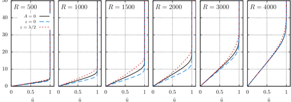
0 10 20 30 40 50 0 0.5 1 y ˜ u A= 0 z= 0 z=λ/2 R= 500 0 10 20 30 40 50 0 0.5 1 y ˜ u R= 1000 0 10 20 30 40 50 0 0.5 1 y ˜ u R= 1500 0 10 20 30 40 50 0 0.5 1 y ˜ u R= 2000 0 10 20 30 40 50 0 0.5 1 y ˜ u R= 3000 0 10 20 30 40 50 0 0.5 1 y ˜ u R= 4000
Figure 3.Evolution of streamwise velocity profiles at both symmetry planesz= 0 andz=λ/2 for the streak amplitude parameter A= 2. The unperturbed boundary layer profiles (A = 0) are added for comparison.
streamwise mass flux are plotted at ten streamwise locations fromR= 300 toR= 3,000. These figures clearly show the sinusoidal spanwise modulation in form of streamwise aligned streaks produced by the finite-amplitude optimal inflow perturbation, which is composed of a pair of counter-rotating vortices (Paredeset al.2016d,c). At the symmetry plane, z = Lz/2, the near-wall, low-momentum fluid is lifted upward by the
counter-rotating vortices, resulting in a localized region of increased boundary layer thickness. At the other symmetry plane, z = 0 (and z = Lz because of spanwise periodicity),
the effect of the initial vortices is exactly the opposite, yielding a localized region of reduced boundary layer thickness. As explained below, the spanwise wavenumber of the relevant first-mode waves is typically smaller than the spanwise wavenumber corresponding to the optimal perturbations. Therefore, the basic state used for the study of interactions between the streaks and important first-mode waves consists of multiple streak wavelengths as shown in figure 2 forλ= 4λST.
Figure 3 displays the comparison of the basic state streamwise velocity profile ¯u(x, y) and total perturbed streamwise velocity profiles u(x, y, z) = ¯u(x, y) + ˜u(x, y, z) at the symmetry planes z = 0 and z = λST for the A = 2.0 case. The differences between
the profiles at both symmetry planes are most visible between R = 1,000 and R = 2,000, which also corresponds to the region with the highest streak amplitudes as shown previously in figure 1(a). Figure 3 also shows the induced spanwise modulation in the boundary layer thickness.
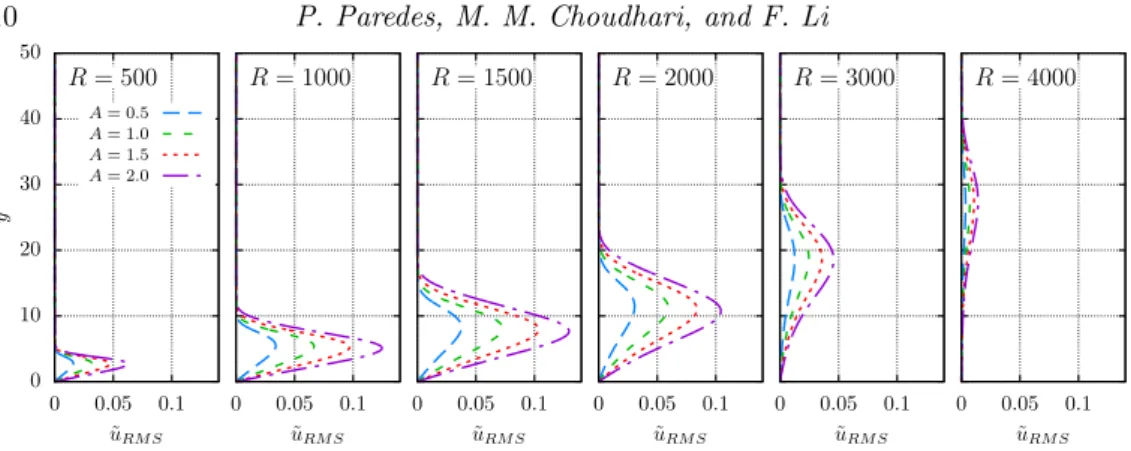
10 P. Paredes, M. M. Choudhari, and F. Li 0 10 20 30 40 50 0 0.05 0.1 y ˜ uRM S A= 0.5 A= 1.0 A= 1.5 A= 2.0 R= 500 0 10 20 30 40 50 0 0.05 0.1 y ˜ uRM S R= 1000 0 10 20 30 40 50 0 0.05 0.1 y ˜ uRM S R= 1500 0 10 20 30 40 50 0 0.05 0.1 y ˜ uRM S R= 2000 0 10 20 30 40 50 0 0.05 0.1 y ˜ uRM S R= 3000 0 10 20 30 40 50 0 0.05 0.1 y ˜ uRM S R= 4000
Figure 4.Evolution of the root-mean-square streamwise velocity, ˜uRM S for selected streak
amplitude parameters, namely,A= 0.5, 1.0, 1.5, and 2.0.
0.95 1 1.05 1.1 1.15 0 1000 2000 3000 4000 5000 cf /cf ( A =0) R A= 0.0 A= 0.5 A= 1.0 A= 1.5 A= 2.0 (a) 0 10 20 30 40 50 60 −4−2 0 2 4 y ˜ uM F D×102 R= 1500 0 10 20 30 40 50 60 −4−2 0 2 4 y ˜ uM F D×102 R= 3000 0 10 20 30 40 50 60 −4−2 0 2 4 y ˜ uM F D×102 R= 4500 (b)
Figure 5.(a) Evolution of spanwise-averaged local skin friction coefficient ratio between those
corresponding to perturbed and unperturbed flows, cf/cf(A=0). Also, (b) M F D streamwise
velocity profiles at streamwise positionsR= 1,500; 3,000; and 4,500.
as ˜ uRM S(x, y) = 1 λST Z λST 0 p u(x, y, z)2− hui(x, y)2dz, (3.2) where hui(x, y) = 1 λST Z λST 0 u(x, y, z)dz, (3.3)
at streamwise locations ofR= 500; 1,000; 1,500; 2,000; 3,000; and 4,000. By comparing the boundary layer profiles in figure 3 and the ˜uRM Sprofiles, the maximum value of ˜uRM S
occurs just below the boundary layer edge along thez= 0 plane.
Finally, the effect of streaks on the skin friction coefficient is studied in figure 5. Figure 5(a) shows the ratio of the spanwise-averaged local skin friction coefficient with respect to that in the unperturbed case (A = 0). A peak skin friction increment of approximately 10% is observed for the A = 2.0 case. For R > 3,800; the skin friction corresponding to A > 0 is lower than that of the unperturbed boundary layer flow. This behavior is explained by the evolution of the mean-flow-distortion (M F D) of the perturbation, ˜qM F D, in figure 5(b). The wall-normal gradient of the streamwise velocity
component of theM F D, ˜uM F D, is positive at the wall forR= 1,500 andR= 3,000; but
3.2. Effect of streaks on first-mode waves
The modal instability of the unperturbed, adiabatic, Mach 3 flat-plate boundary layer flow was examined by Paredeset al.(2016c). By using quasi-parallel LST analysis, they showed that the most amplified instability waves atR= 1,000 correspond to first-mode waves with spanwise wavenumber β ≈0.075 and disturbance frequencyω = 0.02. This spanwise wave number is rather small compared with that corresponding to optimal disturbance initiated near the leading edge and for maximum transient growth at R= 1,000; i.e, βST = 0.25. Following the same approach used here, Paredes et al. (2016c)
presented the spatial evolution of fixed frequency, oblique, first-mode instabilities in terms of the logarithmic amplification ratio based on the energy norm, the so-calledN-factor, as defined by Eq. (2.3). PSE calculations showed that N = 5 is reached atR = 1,596 (i.e.,Rex= 2.55×10⁶) andN = 10 is achieved atR= 3,226 (Rex= 1.04×10⁷).
Herein, the modal instability characteristics of the boundary layer flow perturbed by the finite-amplitude streaks are studied by means of the linear, plane-marching PSE. The three-dimensional basic state is composed of the baseline two-dimensional boundary layer plus the finite-amplitude, linearly optimal perturbation discussed previously. The pair of oblique first-mode waves with equal but opposite wave angle are modulated by the presence of the streaks. For disturbance wavelengths that correspond to λ = λST
(fundamental wavelength) andλ= 2λST (subharmonic wavelength), the symmetric and
antisymmetric modes have different amplification rates. For all other wavelengths, the disturbance field can be decomposed into a pair of modes traveling in opposite directions along the spanwise direction. Both modes in this pair have the same amplification rate in x and their mode shapes satisfy the condition ˆq−(x, y, z) = ˆq+(x, y,−z), where the superscripts + and −denote the signs of the spanwise components of phase velocities associated with the two modes constituting the pair. Because of this, the mode shape for just one of the two waves is presented for those wavelengths.
The results are divided into two groups: highly oblique waves, i.e., first-mode waves with spanwise wavelengths equal to or lower than two streak wavelengths (Section 3.2.1), and nearly planar waves, i.e., first-mode waves with spanwise wavelengths larger than two streak wavelengths (Section 3.2.2). Finally, the overall effect of streaks on the amplification of first-mode waves and the associated transition onset location is presented in Section 3.2.3.
3.2.1. Destabilization of highly oblique waves, λ62λST
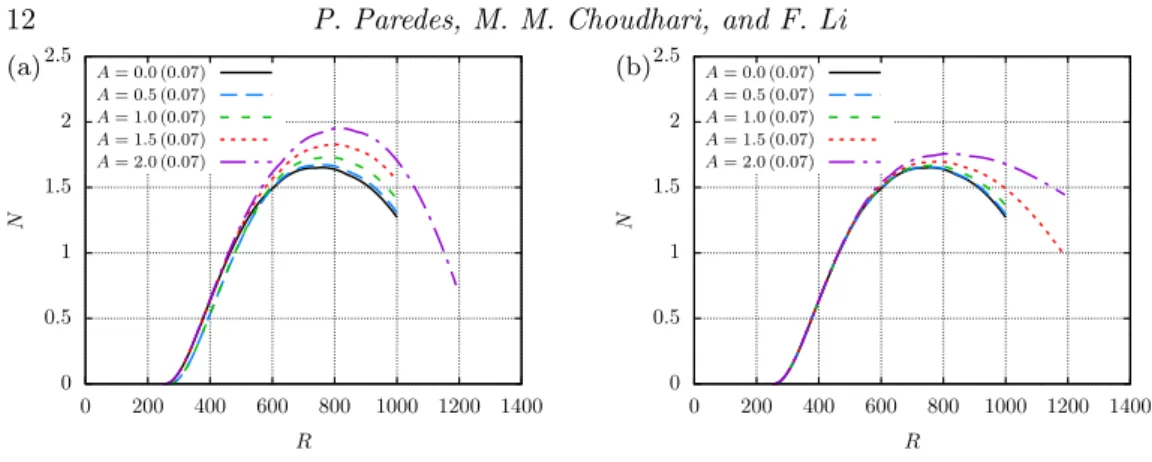
The N-factor envelope evolution for first-mode waves with fundamental spanwise wavelength (λ = λST), are plotted in figures 6(a) and 6(b) for the symmetric and
antisymmetric modes, respectively. The symmetric or antisymmetric character is defined by the structure of the ˆu mode shape with respect to the centerline of the streak (ζ = Lz/2). The N-factor envelopes of figures 6(a) and 6(b) are built upon N-factor
curves with disturbance frequencies ω = 0.05, 0.06, 0.07, and 0.08. The presence of the streaks leads to slight destabilization of both symmetric and antisymmetric first modes at the fundamental spanwise wavelength, but the modulated symmetric modes reach a higher peakN-factor (N ≈2) than the antisymmetric modes. The mode shapes of both antisymmetric and symmetric first-mode waves with fundamental spanwise wavelength are plotted in figure 7 for ω = 0.07, R = 700, and A = 2.0. The real and imaginary parts and the modulus of the streamwise velocity fluctuation of the antisymmetric mode are plotted in figures 7(a), 7(b), and 7(c), respectively. The presence of the streak leads to a concentration of the fluctuation in between the two symmetry planes. Figures 7(d) through 7(f) show analogous mode shapes for the symmetric mode. In this case, the presence of the streak leads to a concentration of the fluctuation over both of the
12 P. Paredes, M. M. Choudhari, and F. Li 0 0.5 1 1.5 2 2.5 0 200 400 600 800 1000 1200 1400 N R A= 0.0 (0.07) A= 0.5 (0.07) A= 1.0 (0.07) A= 1.5 (0.07) A= 2.0 (0.07) (a) 0 0.5 1 1.5 2 2.5 0 200 400 600 800 1000 1200 1400 N R A= 0.0 (0.07) A= 0.5 (0.07) A= 1.0 (0.07) A= 1.5 (0.07) A= 2.0 (0.07) (b)
Figure 6. N-factor envelopes of first-mode waves with fundamental spanwise wavelength,
λ = λST, with (a) symmetric and (b) antisymmetric mode shapes. The selected disturbance frequencies are ω = 0.06, 0.07, 0.08, and 0.09. Note that the most amplified disturbance frequency is specified within parentheses for each streak amplitude parameter.
(a) ℜ(ˆu) 0 5 10 15 y (b)ℑ(ˆu) (c) 0 5 10 15 y (d) ℜ(ˆu) 0 10 20 z 0 5 10 15 y (e) ℑ(ˆu) 0 10 20 z (f) 0 10 20 z 0 5 10 15 y -1 -0.5 0 0.5 1 ℜ(ˆu),ℑ(ˆu) 0 0.5 1 |ˆu|
Figure 7.Isocontours of the (a,d) real and (b,e) imaginary parts and (c,f) modulus of streamwise
velocity fluctuations associated with the (a,b,c) antisymmetric and (d,e,f) symmetric first modes with fundamental wavelength λ = λST and frequency ω = 0.07, at streamwise position
R = 700 and for streak amplitude parameter A = 2.0. The isolines of basic state mass flux ¯
ρu¯= 0.1 : 0.1 : 0.9 are included.
symmetry planes, with the overall maximum along the symmetry plane corresponding to the lower boundary layer thickness,z= 0.
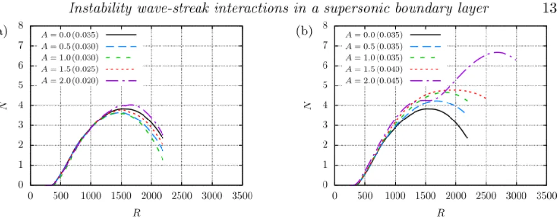
Next, the effect of the streaks on the first-mode waves with subharmonic wavelength (λ = 2λST) is presented. Figure 8(a) and 8(b) show the N-factor envelope curves for
the symmetric and antisymmetric subharmonic modes, respectively. These N-factor envelopes are built upon N-factor curves with disturbance frequencies ω = 0.035, 0.040, 0.045, 0.050, and 0.055. For the subharmonic wavelength, the effect of streaks on the symmetric mode is nonmonotonic with respect to streak amplitude, because the maximumN-factor decreases fromA= 0.0 untilA= 1.0, but theN-factor peak increases again forA= 1.5 andA= 2.0. As shown in figure 8(a), the maximumN-factor for the symmetric modes forA= 2.0 is slightly larger thanN = 4. The figure 8(b) shows that the streaks increase the maximum amplification ratio of the antisymmetric modes. The behavior of the N-factor envelope curve for the A= 2.0 streak is different from that at lower streak amplitudes. Similar to A < 2.0, the N-factor curve for the A = 2.0 case nearly flattens in the vicinity of the upper branch neutral station corresponding to the unperturbed boundary layer. However, the amplification rate does not become negative, and in fact, the antisymmetric modes undergo a new spurt of growth, yielding a peakN -factor value ofN≈6.7 atR≈2,680, which is much larger than theN-factor ofN ≈4.8 at R = 1,960 for A= 1.5. The sudden increase in peak N-factor from A = 1.5 to 2.0
0 1 2 3 4 5 6 7 8 0 500 1000 1500 2000 2500 3000 3500 N R A= 0.0 (0.035) A= 0.5 (0.030) A= 1.0 (0.030) A= 1.5 (0.025) A= 2.0 (0.020) (a) 0 1 2 3 4 5 6 7 8 0 500 1000 1500 2000 2500 3000 3500 N R A= 0.0 (0.035) A= 0.5 (0.035) A= 1.0 (0.035) A= 1.5 (0.040) A= 2.0 (0.045) (b)
Figure 8. N-factor envelopes of first-mode waves with subharmonic spanwise wavelength,
λ= 2λST, with (a) symmetric and (b) antisymmetric mode shapes. The selected disturbance frequencies are ω = 0.020, 0.025, 0.030, 0.035, 0.040, 0.045, and 0.050. Note that the most amplified disturbance frequency is specified within parentheses for each streak amplitude parameter. (a) ℜ(ˆu) 0 5 10 15 y (b)ℑ(ˆu) (c) 0 5 10 15 y (d) ℜ(ˆu) 0 20 40 z 0 5 10 15 y (e)ℑ(ˆu) 0 20 40 z (f) 0 20 40 z 0 5 10 15 y -1 0 1 ℜ(ˆu),ℑ(ˆu) 0 0.5 1 |uˆ|
Figure 9.Isocontours of the (a,d) real and (b,e) imaginary parts and (c,f) modulus of streamwise
velocity fluctuations associated with the (a,b,c) antisymmetric and (d,e,f) symmetric first modes with subharmonic wavelength λ = 2λST and frequency ω = 0.035, at streamwise position
R = 1,000 and for streak amplitude parameter A= 2.0. The isolines of basic state mass flux ¯
ρu¯= 0.1 : 0.1 : 0.9 are included.
represents an onset of streak instability. As shown in Paredeset al.(2016c), at sufficiently large streak amplitudes, the original antisymmetric first mode with subharmonic spanwise wavelength becomes the subharmonic, sinuous (SS) mode of streak instability. By virtue of its high amplification ratios, the SS mode tends to accelerate transition at high streak amplitudes.
The mode shapes of the subharmonic symmetric and antisymmetric modes are com-pared in figure 9 for a disturbance frequency ω = 0.035 at the streamwise location
R = 1,000. The real and imaginary parts and the modulus of the streamwise velocity perturbation for the antisymmetric mode are plotted in figures 9(a), 9(b) and 9(c), respectively; and similar results for the symmetric subharmonic mode are displayed in figures 9(d), 9(e) and 9(f). In the subharmonic case, the fluctuations are concentrated in the region of smaller boundary layer thickness for the antisymmetric mode, and in the region of larger boundary layer thickness for the symmetric mode.
Further analysis of the most amplified instability wave from figure 8(b) is presented in figure 10(a), wherein theN-factor evolution of the subharmonic antisymmetric mode with
ω= 0.045 is compared between theA= 2.0 andA= 0.0 cases. In addition, figure 10(a) also includes the N-factor evolution for two “artificial” basic states: a two-dimensional basic state corresponding to the spanwise average of theA= 2.0 flow, which corresponds to the unperturbed flow (A = 0.0) plus the mean flow distortion (M F D) due to the
14 P. Paredes, M. M. Choudhari, and F. Li
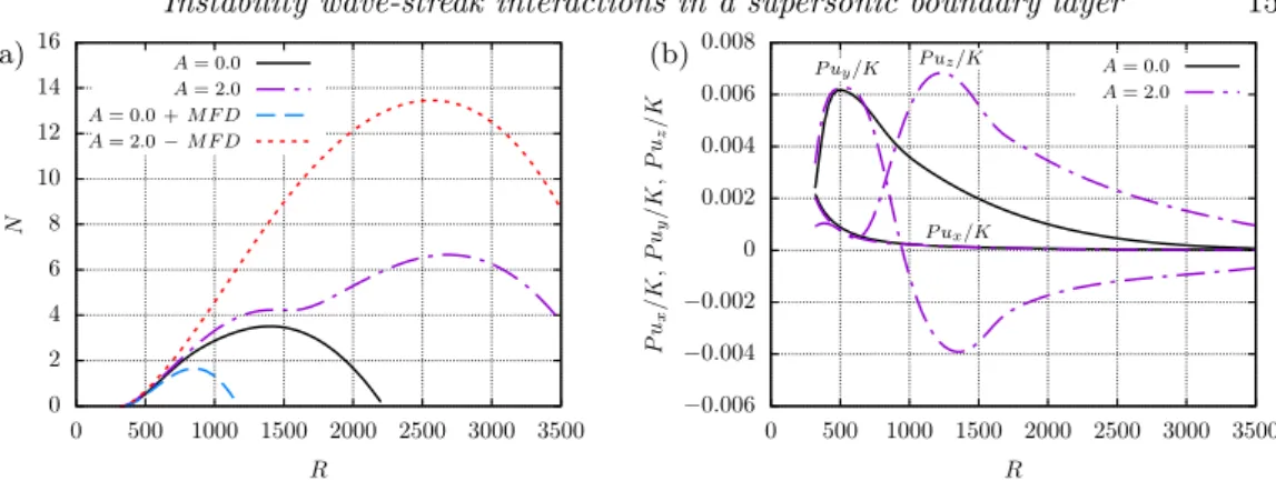
streak, and the perturbed flow withA= 2.0 minus theM F Dof the perturbation. These extra cases are introduced to shed further light on the primary mechanism for the effect of the streak on the enhanced amplification of the first-mode instability. By comparing the N-factor for the first extra case (A = 0.0 +M F D) with that for the unperturbed flow (A= 0.0), we can see that theM F D has a strong stabilizing influence on the first mode. TheN-factor evolution for the second “artificial” case (A= 2.0−M F D) indicates a larger region of amplification relative to the baseline case (A= 0.0), revealing that the previously discussed downstream shift in theN-factor maximum atA= 2.0 is the result of the spanwise gradients of the modified flow. Similar conclusions may be drawn from figure 10(b), which shows the evolution of the normalized production terms (Eq. 2.9) associated with the streamwise velocity gradients, namely,
P ux= Z z Z y Iuxdydz, P uy= Z z Z y Iuydydz, P uz= Z z Z y Iuzdydz, (3.4)
for the subharmonic antisymmetric wave withA= 2.0 and first-mode wave withA= 0.0, andω= 0.045. The production terms are normalized with the disturbance kinetic energy defined by Eq. (2.7). The production terms for the unperturbed boundary layer and the A = 2.0 case are almost coincident at the earlier streamwise stations because the streak amplitudes are small, i.e., Asu < 0.1, for R < 500 (figure 1(a)). As the streak
amplitude becomes relevant forR >500, the wall-normal termP uy/K deviate from the
unperturbed case and becomes negative, which denotes a stabilization effect, and the spanwise termP uz/K notably increases, which denotes a destabilization effect. For the
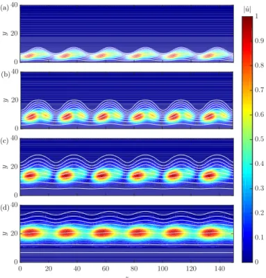
same instability wave, figures 11(a) through 11(d) show the isocontours of the streamwise velocity fluctuation at streamwise locations R = 600; 1,200; 1,800; and 2,400. The concentration of the instability wave peaks on the symmetry plane with reduced boundary layer thickness at the upstream station R = 600, and is successively displaced toward the sides of the centerline symmetry plane (z=λ/2), where the spanwise gradients are larger (Paredes et al. 2016c), indicating a gradual morphing into streak instability. A consequence of this change of the first-mode wave into a streak instability mode, the associated phase speed increases, as well as the amplified frequency range. As indicated by figure 8(b), the most amplified frequency of the antisymmetric subharmonic mode for theA= 2.0 case is larger (ω= 0.045) than forA= 1.5 (ω= 0.040).
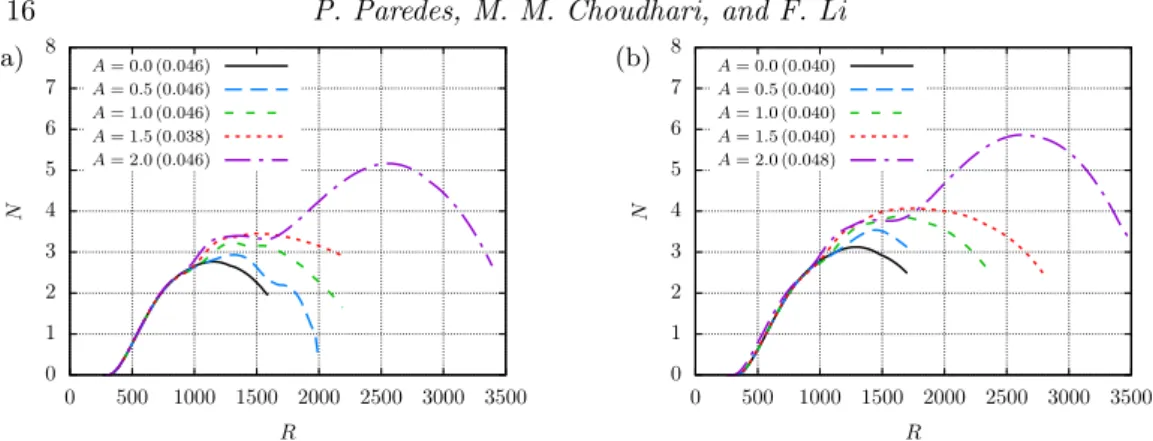
Next, the effect of the streak on first-mode waves with spanwise wavelengths between
λ=λST andλ= 2λST is studied. Figures 12(a) and 12(b) show theN-factor evolution
for first-mode waves with λ = 3/2λST and λ = 5/3λST, respectively. For both cases,
the effect is similar to the antisymmetric subharmonic case (λ = 2λST) of figure 8,
although the N-factor values at every streamwise location remain below the value for the subharmonic case (λ = 2λST) discussed above. An analysis equivalent to figure
figure 10 for the antisymmetric, subharmonic mode is shown for the λ= 5/3λST case
withω= 0.048 in figure 13(a). Similar to the antisymmetric subharmonic case, theM F D
is found to strongly stabilize the first mode, whereas the spanwise gradients destabilize the mode, with the net effect being significantly destabilizing (maxN-factor of 5.9 relative to N ≈3.0 for the baseline case with A = 0.0). Figures 13(b) through 13(f) illustrate the streamwise evolution of the real part of streamwise velocity fluctuation associated with the mode from figure 13(a). AtR= 600 (figure 13(b)), when the streak amplitude is small the three wavelengths of the instability wave are clearly identified within the domain of five streak wavelengths included in the figure. Further downstream, the mode shape becomes more complex and the number of wavelengths becomes hard to identify. Figure 14 shows the evolution of the modulus of the streamwise velocity fluctuation for the same instability wave, i.e., λ = 5/3λST and ω = 0.048. Unlike figure 13(b), the
0 2 4 6 8 10 12 14 16 0 500 1000 1500 2000 2500 3000 3500 N R A= 0.0 A= 2.0 A= 0.0 +M F D A= 2.0−M F D (a) −0.006 −0.004 −0.002 0 0.002 0.004 0.006 0.008 0 500 1000 1500 2000 2500 3000 3500 P ux /K , P uy /K , P uz /K R A= 0.0 A= 2.0 P ux/K P uy/K P uz/K (b)
Figure 10. Analysis of antisymmetric first mode with subharmonic wavelength λ = 2λST
and frequencyω= 0.045 for streak amplitude parameterA= 2.0. (a) Evolution ofN-factors for the unperturbed boundary layer,A = 0.0, the streaky boundary layer with A= 2.0, and two “artificial” basic states: a two-dimensional boundary layer composed by the unperturbed boundary layer, and the M F D of the A = 2.0 case and a three-dimensional boundary layer composed by the boundary layer with A = 2.0 without the M F D of the perturbation. (b) Evolution of the ratio between the crossplane integrals of the production terms associated with the streamwise velocity gradients and the kinetic energy of the perturbation.
(a) 0 10 20 y (b) (c) 0 20 40 z 0 10 20 y (d) 0 20 40 z 0 0.2 0.4 0.6 0.8 1 |ˆu|
Figure 11.Isocontours of the modulus of streamwise velocity fluctuations associated with the antisymmetric first mode with subharmonic wavelengthλ= 2λST and frequencyω= 0.045, at streamwise positions (a) R= 600, (b)R= 1,200, (c)R= 1,800, and (d)R = 2,400, and for streak amplitude parameter A= 2.0. The isolines of basic state mass flux ¯ρu¯= 0.1 : 0.1 : 0.9 are included.
three wavelengths of the disturbance cannot be distinguished in the modulus plot at the same location (figure 14(a)). The fluctuation concentrates around the sides of the streak where the spanwise gradients of ¯uare larger, as previously observed for the antisymmetric subharmonic case in figure 11. Note that, forλ= 5/3λST, the modulus of the fluctuation
is no longer symmetric with respect to the streak symmetry planes. As explained before, for the unperturbed flow there exist two first-mode waves with equal but opposite angles with respect to the free stream. Therefore, forλ6=λST andλ6= 2λST, there is a second
first-mode wave modulated by the streak with an equivalent mode shape corresponding to ˆq−(x, y, z) = ˆq+(x, y,−z), where the superscripts + and − indicate the two waves from a pair.
3.2.2. Stabilization of nearly planar waves, λ >2λST
The effect of streaks on oblique first-mode waves with spanwise wavelengths larger than
16 P. Paredes, M. M. Choudhari, and F. Li 0 1 2 3 4 5 6 7 8 0 500 1000 1500 2000 2500 3000 3500 N R A= 0.0 (0.046) A= 0.5 (0.046) A= 1.0 (0.046) A= 1.5 (0.038) A= 2.0 (0.046) (a) 0 1 2 3 4 5 6 7 8 0 500 1000 1500 2000 2500 3000 3500 N R A= 0.0 (0.040) A= 0.5 (0.040) A= 1.0 (0.040) A= 1.5 (0.040) A= 2.0 (0.048) (b)
Figure 12. N-factor envelopes of first-mode waves with spanwise wavelength equal to (a)
λ= 3/2λST and (b)λ= 5/3λST. The selected disturbance frequencies to build the envelopes are (a)ω = 0.030, 0.038, 0.046, and 0.054, and (b)ω = 0.032, 0.040, 0.048, and 0.056. Note that the most amplified disturbance frequency is specified within parentheses for each streak amplitude parameter. 0 2 4 6 8 10 12 14 16 0 500 1000 1500 2000 2500 3000 3500 N R A= 0.0 A= 2.0 A= 0.0 +M F D A= 2.0−M F D (a) (b) 0 10 y (c) 0 10 y (d) 0 10 y (e) 0 10 y (f) 0 50 100 z 0 10 y -1 -0.5 0 0.5 1 ℜ(ˆu)
Figure 13. Analysis of first mode with spanwise wavelength λ = 5/3λST and frequency
ω = 0.048 for streak amplitude parameter A = 2.0. (a) Evolution of N-factors for the unperturbed boundary layer, A = 0.0, the streaky boundary layer with A = 2.0, and two “artificial” basic states: a two-dimensional boundary layer composed by the unperturbed boundary layer and the M F D of the A = 2.0 case, and a three-dimensional boundary layer composed by the boundary layer with A = 2.0 without the M F D of the perturbation. Also, isocontours of the real part of the streamwise velocity fluctuation at (b)R= 600, (c)R= 800, (d) R = 1,000, (e) R = 1,200, and (f) R = 1,400. The isolines of basic state mass flux ¯
ρu¯= 0.1 : 0.2 : 0.9 are included.
for selected streak amplitude parameters and instability wavelengths of λ = 5/2λST,
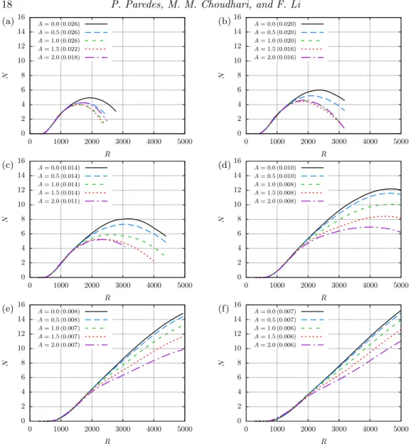
3λST, 4λST, 6λST, 8λST, and 10λST, respectively. For each of these longer spanwise
wavelengths, the introduction of streaks yields a stabilization of the first-mode waves with respect to the unperturbed case (A = 0.0). For λ = 5/2λST (figure 15(a)), λ =
3λST (figure 15(b)), and λ = 4λST (figure 15(c)) the magnitude of stabilizing effect
is not strictly monotonic with respect to increasing streak amplitude. Therefore, there is an optimum streak amplitude for maximum stabilization of the first-mode waves at these spanwise wavelengths. On the other hand, the results for the larger wavelengths in figures 15(d), 15(e) and 15(f) indicate a progressively increasing stabilization effect as the streak amplitude becomes larger.
The relative contributions of the mean flow distortion (M F D) and spanwise variations associated with the streak on the amplification characteristics of instability waves with
(a) 0 10 20 y (b) 0 10 20 y (c) 0 10 20 y (d) 0 20 40 60 80 100 120 z 0 10 20 y 0 0.1 0.2 0.3 0.4 0.5 0.6 0.7 0.8 0.9 1 |ˆu|
Figure 14.Isocontours of the modulus of streamwise velocity fluctuations associated with the first mode with spanwise wavelength λ = 5/3λST and frequency ω = 0.048, at streamwise positions (a) R = 600, (b) R = 1,200, (c) R = 1,800, and (d) R = 2,400, and for streak amplitude parameter A = 2.0. The isolines of basic state mass flux ¯ρu¯ = 0.1 : 0.1 : 0.9 are included.
λ= 6λST are shown in figures 16(a) and 16(b). As previously observed for the
antisym-metric subharmonic case (figure 10(a)) and theλ= 5/3λST case (figure 13(a)), theN
-factor values for theA= 0.0 +M F Dbasic state are much lower than for the rest of basic states. In this case, theN-factor values for theA= 2.0−M F D basic state are slightly larger than those for the unperturbed, two-dimensional boundary layer (A= 0.0). This result indicates that the destabilizing effect of the spanwise gradients is much lower for the long wavelength (λ >2λST) than for the short wavelength modes (λ62λST). Therefore,
the stabilizing effect of the M F D dominates, yielding a significant N-factor reduction for the long wavelength first-mode waves in spanwise modulated boundary layer flow. Figure 16(b) shows that the values of the ratio between the production terms and the kinetic energy are significantly lower than for the subharmonic case of figure 10(b). Here, the lower branch neutral station occurs atR= 650, where the streak amplitude is large enough (Asu= 0.12) to yield larger production terms associated with spanwise gradients
(P uz) than the production termP uy. As the instability wave evolves downstream and
the streak amplitude begins to decrease, the spanwise term P uz/K decreases and the
wall-normal termP uy/K becomes the dominant term atR >3,720.
Figure 17 shows the streamwise evolution of the modulus of streamwise velocity perturbation associated with the instability mode from figure 16. As previously indicated, there exists a pair of waves with the same amplification properties but spanwise-opposite mode shapes that are related via ˜q−(x, y, z) = ˜q+(x, y,−z). The mode shapes of these long wavelength waves are clearly differentiable from the mode shapes from the short wavelength cases in figures 11 and 14 for λ = 2λST and λ = 5/3λST, respectively.
In the short wavelength cases, the concentration of the fluctuation evolved toward the upper part of the boundary layer where the spanwise gradients are larger. In contrast,
18 P. Paredes, M. M. Choudhari, and F. Li 0 2 4 6 8 10 12 14 16 0 1000 2000 3000 4000 5000 N R A= 0.0 (0.026) A= 0.5 (0.026) A= 1.0 (0.026) A= 1.5 (0.022) A= 2.0 (0.018) (a) 0 2 4 6 8 10 12 14 16 0 1000 2000 3000 4000 5000 N R A= 0.0 (0.020) A= 0.5 (0.020) A= 1.0 (0.020) A= 1.5 (0.016) A= 2.0 (0.016) (b) 0 2 4 6 8 10 12 14 16 0 1000 2000 3000 4000 5000 N R A= 0.0 (0.014) A= 0.5 (0.014) A= 1.0 (0.014) A= 1.5 (0.014) A= 2.0 (0.011) (c) 0 2 4 6 8 10 12 14 16 0 1000 2000 3000 4000 5000 N R A= 0.0 (0.010) A= 0.5 (0.010) A= 1.0 (0.008) A= 1.5 (0.008) A= 2.0 (0.008) (d) 0 2 4 6 8 10 12 14 16 0 1000 2000 3000 4000 5000 N R A= 0.0 (0.008) A= 0.5 (0.008) A= 1.0 (0.007) A= 1.5 (0.007) A= 2.0 (0.007) (e) 0 2 4 6 8 10 12 14 16 0 1000 2000 3000 4000 5000 N R A= 0.0 (0.007) A= 0.5 (0.007) A= 1.0 (0.006) A= 1.5 (0.006) A= 2.0 (0.006) (f)
Figure 15. N-factor envelopes of first-mode waves with spanwise wavelength equal to (a)
λ= 5/2λST, (b)λ= 3λST, (c)λ= 4λST, (d)λ= 6λST, (e)λ= 8λST, and (f)λ= 10λST. The selected disturbance frequencies to build the envelopes are (a)ω= 0.018, 0.022, 0.026 and 0.030, (b)ω= 0.012, 0.016, 0.020, 0.024 and 0.028, (c)ω= 0.011, 0.014, 0.017 and 0.020, (d)ω= 0.006, 0.008, 0.010 and 0.012, (e)ω= 0.006, 0.007, 0.008 and 0.009, and (f) ω= 0.005, 0.006, 0.007 and 0.008. Note that the most amplified disturbance frequency within the integration domain is specified within parentheses for each streak amplitude parameter.
the concentration of the fluctuations in the present long wavelength case remains in the interior of the boundary layer.
3.2.3. Overall effect on predicted transition onset
The overall effect of the streaks on the oblique first-mode waves is examined next, in an effort to understand the resulting shift in the transition onset location. Figure 18(a) shows the N-factor envelopes for all spanwise wavelengths considered thus far, namely,
0 2 4 6 8 10 12 14 16 0 1000 2000 3000 4000 5000 N R A= 0.0 A= 2.0 A= 0.0 +M F D A= 2.0−M F D (a) −0.001 −0.0005 0 0.0005 0.001 0.0015 0.002 0 1000 2000 3000 4000 5000 P ux /K , P uy /K , P uz /K R A= 0.0 A= 2.0 P ux/K P uy/K P uz/K (b)
Figure 16.Analysis of first mode with spanwise wavelengthλ= 6λST and frequencyω= 0.010
for streak amplitude parameter A = 2.0. (a) Evolution of N-factors for the unperturbed boundary layer,A= 0.0, the streaky boundary layer withA = 2.0, and two “artificial” basic states: a two-dimensional boundary layer composed by the unperturbed boundary layer and the
M F Dof theA= 2.0 case, and a three-dimensional boundary layer composed by the perturbed boundary layer withA= 2.0 without theM F Dof the perturbation. (b) Evolution of the ratio between the production terms associated with the streamwise velocity gradients and the kinetic energy of the perturbation.
(a) 0 20 40 y (b) 0 20 40 y (c) 0 20 40 y (d) 0 20 40 60 80 100 120 140 z 0 20 40 y 0 0.1 0.2 0.3 0.4 0.5 0.6 0.7 0.8 0.9 1 |uˆ|
Figure 17.Isocontours of the modulus of streamwise velocity fluctuations associated with the first mode with spanwise wavelengthλ= 6λST and frequencyω= 0.010, at streamwise positions (a)R = 1,000, (b) R = 2,000, (c) R= 3,000, and (d)R = 4,000, and for streak amplitude parameterA= 2.0. The isolines of basic state mass flux ¯ρu¯= 0.1 : 0.1 : 0.9 are included.
20 P. Paredes, M. M. Choudhari, and F. Li 0 2 4 6 8 10 12 14 16 0 1000 2000 3000 4000 5000 N R A= 0.0 A= 0.5 A= 1.0 A= 1.5 A= 2.0 (a) 0 2 4 6 8 10 12 14 16 0 1000 2000 3000 4000 5000 6000 7000 N R λ∈[3λST,11λST] λ= 2λST (b)
Figure 18.(a)N-factor envelopes for selected streak amplitude parametersA= 0.0, 0.5, 1.0,
1.5, and 2.0, and spanwise wavelengths within the rangeλ∈[λST,11λST]. (b)N-factor envelope for streak amplitude parameterA= 2.5 separated into destabilized antisymmetric subharmonic modes (λ = 2λST) with frequencies within the range ω ∈ [0.040,0.060] and stabilized long wavelength modes (λ∈[3λST,12λST]) with frequencies within the rangeω∈[0.004,0.024]. (ω∈[0.004,0.090]) for each wavelength. The previously analyzed results are summarized in this plot: the first-mode waves with short wavelengths (λ 62λST), which reach N
-factor values that typically correlate with transition onset location in noisy conditions (N <5) are destabilized, but the first-mode waves with long wavelengths (λ >2λST),
which can reach higher N-factor values that typically correlate with the transition onset location in quiet environments are stabilized. Therefore, the results presented in sections 3.2.1 and 3.2.2 suggest a downstream movement of the transition location in quiet environments, so long as the destabilized subharmonic waves do not cause an earlier onset of transition. These computational findings are not contradictory to the experimental measurements of Holloway & Sterrett (1964) with supersonic boundary layer edge conditions, which showed an upstream movement of the transition location for any roughness height, because of the conventional, i.e., noisy nature of the high-speed facility used in their experiments, which would suggest a likely correlation between the measured transition location and a lowN-factor value (N <5) such as that achieved by short wavelength first-mode waves.
To examine the effect of streak amplitude parameter on transition behavior in benign disturbance environment that corresponds to a transition correlation withN = 10, the
N-factor values of antisymmetric subharmonic modes and for long wavelength waves for a higher streak amplitude parameter case with A = 2.5 are presented in figure 18(b). Paredeset al.(2016c) showed that the antisymmetric subharmonic mode or, equally, the subharmonic sinuous (SS) mode, reachesN = 10 for approximately an streak amplitude parameter value ofA= 2.5. Figure 18(b) shows that the peakN-factor value reached by the SS mode isN = 10.6. The streamwise domain is increased up toR= 7,000 because
N = 10 is reached by the other instability modes atR= 5,116 by the first-mode wave withλ= 11λST andω= 0.005.
Table 1 shows the effect of streak amplitude parameters on the streamwise location,
R, where the selected criticalN-factor values of N = 5, 7 and 10 are reached, and on the frequency, ω, and spanwise wavelength, λ, of the corresponding instability mode. ForA= 1.0, the transition location moves downstream with respect to the unperturbed case. The instability wave that first reaches either of the critical N-factor values has a lower frequency and a larger wavelength than the first-mode wave corresponding to the unperturbed basic state withA= 0.0. For a larger streak amplitude parameter ofA= 2.0, the SS mode reachesN = 5 earlier than the long wavelength first-mode waves, although
A N= 5 N = 7 N = 10 R ω λ(×λST) R ω λ(×λST) R ω λ(×λST) 0.0 1656.4 0.0254 3 2299.4 0.0175 4 3247.4 0.0113 6 1.0 1791.4 0.0164 4 2634.0 0.0106 6 3698.6 0.0080 8 2.0 1911.8 0.0459 2 3328.7 0.0072 8 4597.2 0.0059 10 2.5 1742.3 0.0548 2 2035.6 0.0593 2 2607.5 0.0592 2
Table 1. Effect of streak amplitude parameters on the streamwise location, R, where the
selected N-factors are reached and on the properties of the corresponding first-mode wave, namely, the disturbance frequency,ω, and spanwise wavelength,λ. Note that numbers in bold font refer to the destabilized antisymmetric subharmonic mode (λ= 2λST).
farther downstream than theλ= 4λST wave forA= 1.0. The frequency associated with
the SS mode is much larger than the frequency associated with the λ= 4λST wave for A = 1.0. The trend of decreasing frequency and increasing wavelength observed from
A = 0.0 to A = 1.0 is also observed from A = 1.0 to A = 2.0 for the largerN-factor values of N = 7 and 10. The last row of Table 1 shows the transition location and the properties of the SS mode wave that is the first to reachN-factor values up toN = 10 as shown in figure 18. As shown by Paredeset al.(2016c), the most amplified frequency associated with the SS mode increases with the streak amplitude, which is in agreement with the increase in N = 5 frequency from ω = 0.0459 at A = 2.0 to ω = 0.0548 at
A= 2.5.
The overall effect of the streaks on the instability characteristics of the supersonic boundary layer flow is summarized in figure 19(a), where the transition location cor-responding to selected N-factor values is plotted as a function of the computed streak amplitude parameters, A. Figure 19(b) shows the same results but normalized with the unperturbed case to reflect the relative displacement of the transition location. Selecting
N = 5 as the transition threshold, figure 19(a) shows how the transition onset due to first-mode waves would be slightly displaced downstream by the introduction of the optimal streaks. However, forA>2, the SS mode reachesN = 5 at a position upstream of the larger wavelength modes stabilized by the streaks; this leads to an upstream shift in transition location relative to the baseline (A= 0.0) case. For larger N-factor values, the streaks yield a significant downstream movement of the transition onset location, as long as the streak amplitude is below a threshold value to avoid an early transition onset due to the SS mode. Figure 19(b) shows that for the present configuration, the streaks at any specified value ofA produce the maximum relative shift in transition location when
N = 8. Nevertheless, the trend in transition location from figure 19(b) is quite similar for allN>6. Therefore, the interaction of the streaks with the first-mode instability waves results in a net stabilization of nearly planar waves, yielding a significant transition delay in quiet environments for which the onset of transition typically correlates withN ≈10. The present results show a potential increase in the length of the laminar flow that is comparable to the length of the laminar region in the unperturbed case, i.e., the laminar flow acreage is potentially doubled. Considering that the ratio of local skin friction coefficients for turbulent and laminar flows is in the range ofcf,tur/cf,lam∈[3,5]
for a flat-plate boundary layer with an edge Mach number of 3 (Schlichting 1979), the total skin friction reduction for a flat plate with a total length corresponding toRel=
25×106, at the present flow conditions (M = 3, Re0 = 106/m) and with a transition threshold ofN = 10, would be of the order of the 50−70% relative to the unperturbed case. A parameter study for additional streak wavenumbers and excitation locations, as
22 P. Paredes, M. M. Choudhari, and F. Li 0 0.5 1 1.5 2 2.5 3 0 5 10 15 20 25 30 A Rex=R2(×106) N= 5 N= 6 N= 7 N= 8 N= 9 N= 10 FM SI (a) 0 0.5 1 1.5 2 2.5 3 0 0.5 1 1.5 2 2.5 3 A Rex/Rex(A= 0) (b)
Figure 19. Effect of streak amplitude parameterAon transition location based on N factor
valuesN = 5, 6, 7, 8, 9, and 10. Note that solid lines with filled symbols refer to stabilized long wavelength modes (λ > 2λST) and dashed lines with open symbols refer to destabilized antisymmetric subharmonic modes (λ= 2λST).
well as suboptimal streak profiles that are more readily realizable via the available set of actuation techniques, would be very helpful with identifying the optimal flow control settings that would enable a robust performance with maximum transition delay for a given flow configuration.
4. Conclusions
Optimal growth theory based on parabolized stability equations (PSE), or equivalently, boundary region equations, is used to identify the range of modulating wavelengths that would benefit the most from the intrinsic “lift-up” mechanism within the boundary layer flow. Furthermore, the nonlinear plane-marching PSE are used to predict the downstream development of finite-amplitude, optimal, stationary disturbances introduced near the leading edge. Subsequently, the linear stability characteristics of the perturbed streaky boundary layer flow are studied using the linear form of plane-marching PSE. Results show that stationary streaks lead to a substantial reduction in the amplification of targeted first-mode waves when the streak spacing is less than the spanwise scale of those waves by a factor of two or greater. Instability waves with spanwise wavelengths of twice the streak spacing or lower are destabilized by the streaks; but up to a certain threshold, their amplification factors are sufficiently lower than those of the most amplified waves in the uncontrolled flow so that a significant net stabilization is achieved, yielding a downstream movement of the laminar-turbulent transition onset that is comparable to the uncontrolled transition length. Considering that the wavelengths of the first-mode waves that are substantially amplified in an unperturbed boundary layer flow are much longer than optimal growth streaks, a favorable situation for transition delay is feasible. Furthermore, a detailed analysis has shown that theM F Dof the nonlinear stationary streak perturbation is responsible of the stabilizing effect, while the spanwise variations destabilize the first-mode waves. When the spanwise wavelength of the instability waves is equal to or smaller than twice the streak wavelength, the spanwise production terms dominate and yield the destabilization with respect to the unperturbed case. When the streak amplitude is large enough, the antisymmetric subharmonic mode, becomes the subharmonic, sinuous (SS) mode of streak instability (Paredeset al.2016c), and because of its high amplification ratio, it can lead to the early onset of transition. When the spanwise wavelength of the first-mode waves is larger than twice the streak wavelength, the difference between both spanwise length scales reduce the destabilizing effect of
the spanwise gradients and the streak effects on first-mode waves is dominated by the stabilizing effect of theM F D.
The results indicate that the overall effect of streaks on first-mode instabilities may result in a notable transition delay if suitable stationary disturbances can be excited in the flow. The base flow modulation at the required wavelengths and amplitudes can be generated by using micro vortex generators or discrete roughness elements. However, the growth characteristics and profiles of the streaks generated in this manner will be different from those excited via optimum initial conditions. The realizability of such initial disturbances and/or the effect of realizable but suboptimal disturbances on the first-mode instabilities are part of our ongoing work.
Acknowledgments
This research was sponsored by NASA’s Transformational Tools and Technologies (TTT) Project of the Transformative Aeronautics Concepts Program under the Aero-nautics Research Mission Directorate. Resources supporting this work were provided by the NASA High-End Computing (HEC) Program through the NASA Advanced Supercomputing (NAS) Division at Ames Research Center.
REFERENCES
Andersson, P., Brandt, L., Bottaro, A. & Henningson, D.S.2001 On the breakdown of
boundary layer streaks.J. Fluid Mech.428, 29–60.
Andersson, P., Henningson, D.S. & Hanifi, A.1998 On a stabilization procedure for the
parabolic stability equations.J. Engng. Math.33, 311–332.
Bagheri, S. & Hanifi, A.2007 The stabilizing effect of streaks on Tollmien-Schlichting and oblique waves: a parametric study.Phys. Fluids19, 078103–1–078103–4.
Boiko, A.V., Westin, K.J.A., Klingmann, B.G.B., Kozlov, V.V. & Alfredsson, P.H.
1994 Experiments in a boundary layer subjected to free stream turbulence. Part 2. The rhole of TS-waves in the transition process.J. Fluid Mech.281, 219–245.
Broadhurst, M. & Sherwin, S. 2008 The parabolised stability equations for 3D-flows:
implementation and numerical stability.Appl. Num. Math.58(7), 1017–1029.
Chang, C.-L. & Malik, M.R. 1994 Oblique-mode breakdown and secondary instability in
supersonic boundary layers.J. Fluid Mech.273, 323–360.
Choudhari, M., Li, F., Chang, C.-L., Norris, A. & Edwards, J.2013 Wake instabilities
behind discrete roughness elements in high speed boundary layers. AIAA Paper 2013-0081.
Choudhari, M., Li, F. & Edwards, J.2009 Stability analysis of roughness array wake in a high-speed boundary layer. AIAA Paper 2009-0170.
Cossu, C. & Brandt, L.2002 Stabilization of Tollmien-Schlichting waves by finite amplitude
optimal streaks in the Blasius boundary layer.Phys. Fluids14(8), L57–L60.
De Tullio, N., Paredes, P., Sandham, N.D. & Theofilis, V. 2013 Laminar-turbulent
transition induced by a discrete roughness element in a supersonic boundary layer. J. Fluid Mech.735, 613–646.
Fasel, H., Thumm, A. & Bestek, H. 1993 Direct numerical simulation of transition in
supersonic boundary layer: oblique breakdown. InTransition and Turbulent Compressible Flows (ed. L.D. Kral & T.A. Zang),FED, vol. 151, pp. 77–92. ASME.
Fransson, J.H., Talamelli, A., Brandt, L. & Cossu, C. 2006 Delaying transition to
turbulence by a passive mechanism.Phys. Rev. Lett.96, 064501.
Haj-Hariri, H.1994 Characteristics analysis of the parabolized stability equations.Stud. Appl. Math.92, 41–53.
Hermanns, M. & Hern´andez, J.A.2008 Stable high-order finite-difference methods based on
non-uniform grid point distributions.Int. J. Numer. Meth. Fluids 56, 233–255.
Holloway, P.F. & Sterrett, J.R.1964 Effect of controlled surface roughness on boundary-layer transition and heat transfer at Mach number of 4.8 and 6.0. NASA TR-D-2054.