Global Instability Analysis of Laminar Boundary Layer Flow Over a Bump at Transonic Conditions

(1)

Procedia IUTAM 14 ( 2015 ) 503 – 510

Selection and peer-review under responsibility of ABCM (Brazilian Society of Mechanical Sciences and Engineering) doi: 10.1016/j.piutam.2015.03.080

ScienceDirect

IUTAM ABCM Symposium on Laminar Turbulent Transition

Global instability analysis of laminar boundary layer ﬂow over a

bump at transonic conditions

Jos´e Miguel P´erez

a,∗

_{, Pedro Paredes}

a

_{, Vassilis Theoﬁlis}

a

a_{School of Aeronautics, Universidad Polit´eecnica de Madrid, Plaza Cardenal Cisneros 3, E-28040 Madrid, Spain}

Abstract

Modal three-dimensional BiGlobal linear instability analysis is performed in steady, spanwise-homogeneous two-dimensional laminar compressible boundary-layer flow past a millimeter-tall hemispherical bump at transonic conditions. Starting with subsonic inlet flow, at the flow conditions considered a stationary shock is formed near the downstream end of the bump. The interplay of shock and adverse-pressure-gradient results in a steady spanwise homogeneous laminar two-dimensional laminar separation bubble being formed at the downstream end of the bump.

The objective of the present analysis is to interrogate this basic flow with respect to its potential to sustain low-frequency unsteadiness arising from linear amplification of unstable traveling global flow eigenmodes. Such unsteadiness, coupled to eigen-frequencies of the structure, can lead to resonance phenomena that are detrimental for the performance and adversely affect the efficiency of systems on which the bump configuration is employed. Only damped global eigenmodes have been identified at the parameters examined, pointing to the possibility of the above mentioned unsteadiness being the result of algebraic instability.

c

2014 The Authors. Published by Elsevier B.V.

Selection and peer-review under responsibility of ABCM (Brazilian Society of Mechanical Sciences and Engineering).

Keywords: Shock wave - boundary layer interaction; transonic and supersonic ﬂows; global linear instability

Nomenclature

hbump Bump height

Lbump Bump width

L Length of computational domain

H Height of computational domain

ξ0 Stagnation value of variableξ

ξ∞ Free-stream value of variableξ

ˆ

ξ Amplitude perturbation of variableξ

∗_{Corresponding author. Tel.:}₊_{34 91 336 32 97} E-mail address:josemiguel.perez@tupm.es

(2)

1. Introduction

Shock-wave laminar boundary layer interactions (SWLBLI) are present on aerodynamic systems in the transonic and supersonic regimes. Enhance by the presence of flow separation, SWLBLI may produce low-frequency unsteadi-ness which can be coupled to eigenfrequencies of the structure and lead to resonance phenomena that are detrimental for the performance and adversely affect the efficiency of such systems. Flow instability analysis may shed light on the origin of this interaction processes. However the geometrically complex nature of the surfaces on which SWLBLI typically appears (wedges,λ−shaped shock waves impinging upon the boundary layer, etc) has mostly confined such analysis efforts to idealized regions of the flow, on which classic local instability analysis could be employed3_.

Two types of flow configurations have been used in the literature in order to investigate transonic flow over bumps: those in confined channels and bumps in open channels. The difference between these configurations is that in the former case reflections exist at the top walls. In addition, two different types of bumps are mostly considered in the literature: a variable-curvature bump (the so-calledDelery bump1

geometry) as well as a circular-arc or hemispherical bump geometry2_{. Finally, most studies consider application-related, high Reynolds numbers. For example Batten et}

al.11 _{used RANS model in order to study a ﬂow over the Delery bump while Sandham et al.}10 _{used LES in the}

case of a flow over a circular bump. In all cases, a strong normal shock impinges on the bump and is modified by the interaction with the geometry in inviscid flow and, additionally, with the boundary layer, when viscosity is considered, adopting the well-knownλpattern. In the latter case, the interaction causes separation of the boundary layer and a low-speed recirculating bubble is observed near the shock foot. The flow perturbations that arise in this problem are characterized by two distinct frequencies: a low frequency related with the slow motion of the shock, and a high frequency that appears in the mixing layer where the effects of the shear stress are most relevant. An idealization of the latter problem, which considered shock curvature has been studied by Duck et al.3using classic local linear stability analysis.

The present effort focuses on the stability analysis of a freestream channel with a millimeter hemispherical bump with maximum height of 10 % of the bump width, where the Reynolds number is small and the flow is laminar. Advances in global linear instability analysis6_{over the last decade permit commencing the analysis of SWLBLI flows.}

In addition, the successful work of Crouch and co-workers8regarding the origin of buﬀeting over a two-dimensional airfoil at transonic ﬂight conditions lends credibility to the followed approach.

2. Problem formulation

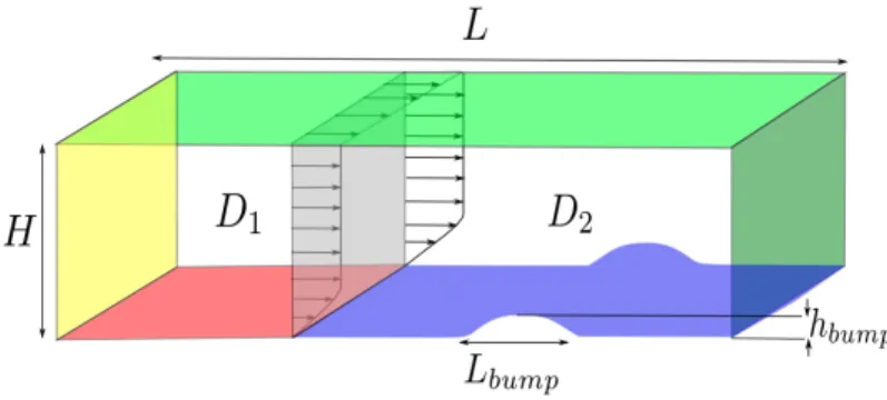
The geometry of the problem consists of a ﬂat plate with a two-dimensional cylindrical bump element that is homogeneous in the spanwise direction. A schematic representation of the geometry and the boundary conditions employed for the computation of the basic state are shown in Figure 1. Zero-pressure-gradient ﬂow of a Newtonian

Fig. 1. Computational domain and boundary conditions: Dirichlet inlet ﬂow (yellow/left wall), freestream (green / top and right walls), adiabatic and slip wall (red / bottom wall inD1) and adiabatic and non-slip wall (blue / bottom wall inD2).

(3)

computational domain isx∈[−1,4]×y∈[0,1.5] in millimeters. The size of the circular-arc bump is defined by its length,Lbump=10−3mand height,hbump=10−4m. Quantities are made dimensionless using the bump length (Lbump), while temperature (T∞), velocity (U∞), density, (ρ∞) and dynamic viscosity, (μ∞) scales are defined at their respective freestream values. Thex-axis is taken to be along the streamwise direction,yis the wall-normal direction and thez -axis is the spanwise direction. The dimensionless quantities obtained using the above scales imply that low-Reynolds number laminar boundary layer flow ensues.

The domain is divided in two regions;D1andD2(see Figure 1). Base ﬂow calculations are performed inD1andD2

while stability analysis is only performed inD2. Inviscid velocity and adiabatic temperature boundary conditions are

considered at theD1(red) wall, while viscous velocity and adiabatic temperature boundary conditions are considered

at theD2(blue) wall. Freestream boundary conditions are considered at the top and outﬂow boundaries (green); an

analogous model proposed by Poinsot and Lele4_{has been used in this respect.}

2.1. Navier-Stokes equations

The non-dimensional compressible Navier-Stokes equations are given by, ∂ρ ∂t +∇ ·(ρu)=0, (1) ∂(ρu) ∂t +∇ ·(ρuu)=− 1 γM2∇p+ 1 Re∇ ·σ , (2) ∂p ∂t +u· ∇p+γp∇ ·u= γ RePr∇ ·(κ∇T)+ γ(γ−1)M2 Re Φ, (3)

whereu= (u,v,w) are the three component velocities,pis the pressure,T the temperature,σis the viscous stress tensor of a Newtonian ﬂuid and

Φ =1 2

∇u+∇uT:σ , (4)

is the dissipation function. Here μandκ are the dynamic viscosity and thermal conductivity, respectively. These quantities could be obtained from the Sutherland’s formula,

μ=C1

T3/2

T+C2 ,

(5) and the relationship betweenμandκis

κ=μcp/Pr, (6)

where cp is the speciﬁc heat at constant pressure and Pr is the Prandtl number. The parameters used areC1 =

1.458×10−6kg/(ms√K), C2 = 110.4K andPr = 0.72; see Schlichting7 for more detail. The non-dimensional

parameters of the problem are the Reynolds numberRe=ρ∞L∞U∞/μ∞and the Mach numberM∞=U∞/√γRT∞.

3. Base ﬂow

The two-dimensional compressible Navier-Stokes equations were solved using the modulerhoCentralFoam within the open-source CFD software OpenFOAM. This module is a density-based compressible ﬂow solver, which uses the central-upwind schemes of Kurganov and Tadmor5_{and an unstructured collocated mesh with a ﬁnite volume}

method. In order to resolve the boundary layer, the grid points were clustered towards the wall in the normal direction. Finer mesh was also used on the bump surface in the streamwise direction clustering points near to the leading and trailing edges of the bump. Away from the bump, the mesh expands in the streamwise direction towards the inflow and outflow boundaries with an aspect ratio close to one. The base flow computational mesh comprises a total number of approximately 2×105_{cells, while computations were performed in parallel on 8 cores.}

A steady base ﬂow atRe=1380 andM=0.675 at the inlet boundary was calculated, usingρ∞=1.2kg/m3,U∞= 229.5m/sandμ∞=2×10−4kg/(ms). Convergence of the base ﬂow was attained using around 550 control volumes in thex-direction and 300 control volumes in the normal direction, obtaining results such as those shown in Figure 3. No

(4)

wave reflections were observed at the top and outflow boundaries during the numerical simulations. Figure 2 shows in semi-logarithmic scale the evolution of the relative error (defined using the transient and the converged values) of the streamwise base flow velocity component at a given point in the flow field, close to the laminar separation bubble. The relative error drops to∼ −14 at 5×10−4_s_{, which corresponds to 23 times the characteristic residential time of the}

ﬂow. -16 -14 -12 -10 -8 -6 -4 -2 0 210-4 410-4 610-4 810-4 Time

Fig. 2. Logarithm of relative error ofU(x=1.5,y=0.5) versus time.

Iso-contours of streamwise and transverse base flow velocity components,UandV, and Mach number are shown in Figure 3 were a peak ofM=1.4 is observed. The bump is placed inside the flat-plate boundary layer, but is actually quite large compared with the characteristic dimension of the boundary layer: the displacement thickness at the inflow and outflow boundaries are, respectively,δ∗_inflow =0.5hbumpandδ∗_outflow =1.0hbump. A small recirculation bubble is

observed in this configuration, as shown in Figure 4. Figure 5 (left)shows the variation of the skin friction coefficient along the bump surface. The friction coefficient decreases at the leading edge of the bump and then increases up to the shock position. This coefficient drops suddenly across the shock and becomes negative. Flow separation exists in this region. Reattachment occurs in a two-dimensional sense when the skin friction is again positive. Progressively the skin-friction coefficient gradually increases downstream. The streamwise velocity component profile at the leeside foot of the bump is shown in Figure 5 (right), where weak recirculation is observed.

Fig. 3. Steady two-dimensional laminar base ﬂow:Uvelocity and streamlines (left),Vvelocity in dimensions variables (middle)and Mach number contours (right).

(5)

Fig. 4. Detail of the recirculation bubble, withUreverse≈ −2%U∞. Base ﬂow streamlines are shown at the leeside foot of the bump. -50 0 50 100 150 200 250 300 350 400 450 500 0 0.5 1 1.5 2 2.5 3 3.5 4 cf 103 x 0 0.0002 0.0004 0.0006 0.0008 0.001 0.0012 0.0014 0.0016 -50 0 50 100 150 200 250 300 350 400 450 y U U 0 5e-06 1e-05 1.5e-05 2e-05 2.5e-05 3e-05 3.5e-05 -4 -2 0 2 4 6

Fig. 5. (Left:)Skin friction coeﬃcient and (Right:)Streamwise velocity componentU(y) at this location.

4. Global Linear Stability Analysis

Global linear stability theory studies the temporal evolution of small amplitude disturbances superimposed upon a base ﬂow6_{. Flow is decomposed into a steady base ﬂow} _Q ₌ ₍_{ρ, ρ}_u_{, ρ}_v_,_E_{), where} _E_{is the total energy, and a}

three-dimensional unsteady small perturbationq, ∂q ∂t = ∂f(Q) ∂q q ≡Aq, (7)

whereAis the Jacobian matrix of the right-hand-side of the Navier-Stokes equations (1-3). According to the BiGlobal Ansatz, solution of the equation (7) are sought as eigenmodes:

q(x,y,z,t)=ˆq(x,y)ei(βz−ωt)+c.c. (8) where1,β=2π/Lzis the wavenumber in the spanwise spatial direction,z,ˆqare the eigenvectors andω=ωr+i·ωi whereωrrepresenting the circular frequency andωibeing the ampliﬁcation/damping rate of the disturbances. A large-scale non-Hermitian generalized eigenvalue problem is obtained, by inserting equation (8) into equation (7),

Aqˆ(x,y)=ωBqˆ(x,y). (9) A shift-and-invert implementation of the Arnoldi algorithm was employed in order to recover a window of the eigenspectrum centered around the shift parameterσ,

ˆ

AX=μX, where ˆA=(A−σB)−1B, μ= 1

(6)

where A andBare a matrix representation for a given discretization of the operators deﬁned in (9) for a given appropriate boundary conditions. The linear algebra work was performed using the sparse MUltifrontal Massively Parallel Sparse direct Solver (MUMPS) package9_{. This was ﬁrst successfully employed to global linear instability}

problems by Crouch et al.8_. 5. Results

The eigenvalue problem (10) derived from the BiGlobal stability analysis was solved numerically using ﬁnite-diﬀerence discretization of 6th order withN x=501 andNy= 301 discretization points. Transformation functions were used in order to follow the geometry variations and cluster points in the vicinity of the wall and the bump ends. This involved using general transformation coordinate as well as metrics in the linearized Navier-Stokes equations, see reference12_{for more details.}

The computational domain considered in the stability analysis corresponds to the regionD2 in Figure 1. The

boundary conditions used for the perturbations variables were homogeneous Dirichlet at the inflow and wall, and homogeneous Neumann at the outflow and top boundaries, with the exception of the density component which satisfies the linearized continuity equations at the walls.

-4

-3.5

-3

-2.5

-2

-1.5

-1

-0.5

0 -1

-0.5

0

0.5

1

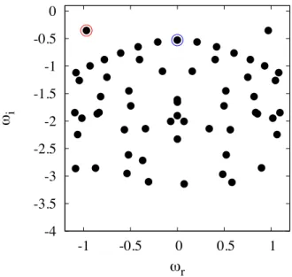
i

_r

Fig. 6. BiGlobal eigenspectrum atRe=1380,M=0.675,β=1.

Figure 6 shows the eigenspectrum corresponding toRe = 1380, M = 0.675 andβ = 1 where the least damped eigenvalue is a traveling perturbation (and its complex-conjugate), marked with a red circle (marked left eigenvalue). The next stronger damped eigenmode is a stationary perturbation, marked with a blue circle (marked right eigen-value). Analogous eigenspectrum structure appears for any of the examined values ofβ∈[0,4π]. Convergence of the leading eigenvalue was attained using different domain lengths in thex-direction, as well as a larger number of dis-cretization points. Iso-contours of the module of the spanwise perturbation velocity amplitude function and amplitude function of the temperature perturbation of the leading traveling and stationary eigenmodes are shown in Figures 7 and 8, respectively. These perturbations are concentrated around the shock and the boundary layer downstream of the bump. Finally, a three-dimensional reconstruction of thetotalspanwise velocity and temperature fields, as obtained from the base flow and a linearly-small amount of the respective eigenmodes is shown in Figure 9. The potential three-dimensionalization of the reattachment region and the subsequent growth inxof linear, spanwise periodic per-turbations is evident in these results. Of particular interest is the adequate resolution of the perturbation around the shock region, evident in the temperature field reconstruction.

(7)

Fig. 7. Values of||Wˆ||and||Tˆ||of the leading stationary mode atRe=1380,M=0.675 andβ=1.

Fig. 8. Values of||Wˆ||and||Tˆ||of one of the leading traveling modes atRe=1380,M=0.675 andβ=1.

Fig. 9. Total ﬂow ﬁeld reconstruction of the spanwise velocity (left) and temperature (right) of the leading stationary mode atRe=1380,M=0.675 andβ=1.

(8)

6. Conclusions

Linear three-dimensional instability analysis of laminar transonic over a circular-arc bump inside a boundary layer has been investigated. Modal global perturbations have been unraveled, peaking in the separated ﬂow region down-stream of the bump. Parametric sweeps inβhas shown that the two-dimensional laminar basic ﬂow at these conditions is stable to both two- and three-dimensional modal perturbations. Consequently, transient growth analysis of the same geometry is presently being pursued.

7. Acknowledgments

Support of the Spanish Ministry of Science and Innovation through Grant TRA34148 (Plan Nacional 2012-2015) is gratefully acknowledged..

References

1. Delery, J.M., “Experimental investigation of turbulence properties in transonic shock/boundary-layer interactions,”,AIAA Journal21(2), 180185, 1983

2. Liu, X., Squire, L.C., “An investigation of shock boundary-layer interactions on curved surfaces at transonic speeds,”,Journal of Fluid Mechan-ics187, 467486, 1987

3. Duck, P. W., Lasseigne, D. J. and Hussaini, M. Y. “The eﬀect of three-dimensional freestream disturbances on the supersonic ﬂow past a wedge”,

Phys. Fluids,9, 456, 1997

4. Poinsot, T. J. Lele, S. “Boundary conditions for direct simulations of compressible viscous ﬂow”,J. Computational Physics,101, 104-129, 1992 5. Kurganov A. and Tadmor E., “New high-resolution central schemes for nonlinear conservation laws and convection diﬀusion equations,”,

Journal of Computational Physics,160(1), 241-282, 2000

6. Theoﬁlis, V. “Global linear instability”,Annual Reviews of Fluid Mechanics,43, 319-352, 2011 7. Schlichting H. “Boundary layer theory”,McGraw-Hill, 1979, 7th

8. Crouch, J. D. and Garbaruk, A. and Magidov, D., “Predicting the onset of ﬂow unsteadiness based on global instability”,J. Comp. Phys.2242, 92494, 2007

9. Amestoy, P. R. and Duﬀ, I. S. and L’Excellent, J.-Y. and Koster, J., “A fully asynchronous multifrontal solver using distributed dynamic scheduling”,SIAM Journal of Matrix Analysis and Applications.1, 1541, 2001

10. Sandham, N.D. and. Yao, Y.F. and Lawal, A.A., “Large-eddy simulation of transonic turbulent ﬂow over a bump”,International Journal of Heat and Fluid Flow24, 584595, 2003

11. Batten, P. and. Craft, T.J. and Leschziner, M.A. and Loyau, H., “Reynolds- stress-transport modeling for compressible aerodynamics applica-tions.”AIAA Journal37(7), 785797, 1999

12. Paredes, P. “Advances in global instability computations: from incompressible to hypersonic ﬂow”,PhD Thesis, Technical University of Madrid, 2014