Contributions to the Sixth Drag Prediction Workshop Using
Structured, Overset Grid Methods
James G. Coder∗
University of Tennessee, Knoxville, Tennessee 37996 David Hue†
ONERA—The French Aerospace Lab, 92190 Meudon, France
Gaetan Kenway‡
University of Michigan, Ann Arbor, Michigan 48109 Thomas H. Pulliam§
NASA Ames Research Center, Moffett Field, California 94035 and
Anthony J. Sclafani,¶Leonel Serrano,**and John C. Vassberg††
Boeing Commercial Airplanes, Long Beach, California 90808 DOI: 10.2514/1.C034486
Structured-grid solutions obtained for the NASA Common Research Model for the Sixth AIAA Computational Fluid Dynamics Drag Prediction Workshop are detailed. Three different flow solvers were used among the contributors, and the numerical methodologies and turbulence modeling strategies employed by each code are described. Key results for all authors include grid convergence studies for the drag increment of a nacelle and pylon added to a wing–body configuration and a buffet study accounting for static aeroelastic deformation. Additional studies performed include feature-based adaptive mesh refinement and higher-order convective flux discretization, among others.
Nomenclature
= wing aspect ratio
b = wing span CD = drag coefficient CL = lift coefficient CM = pitching-moment coefficient Cp = pressure coefficient c = chord length M = Mach number
N = total number of grid points
Re = Reynolds number based on reference chord length
S = wing area
x = x-coordinate direction
y = y-coordinate direction
α = angle of attack
η = nondimensional spanwise coordinate,2y∕b
Subscripts
ref = geometric reference values
∞ = free-stream conditions
I. Introduction
T
HE AIAA Drag Prediction Workshop (DPW) series was first organized to assess the state-of-the-art in computational fluid dynamics (CFD) methods for predicting aircraft forces and moments, to provide a forum for evaluating the effectiveness of codes and modeling techniques, and to identify areas for improvement. The first DPW was held in Anaheim, CA, in 2001, and the 6th and most recent workshop was held in June 2016 in conjunction with the 34th AIAA Applied Aerodynamics Conference in Washington, DC.The focus of the Sixth DPW (DPW-6) [1] is the Common Research Model (CRM), pictured in Fig. 1, which was designed in cooperation by Boeing and NASA to be an open-source commercial transport configuration [2]. The CRM was also used for the 4th and 5th DPWs [3,4] in 2009 and 2012, respectively. In DPW-4, participant simulations of the CRM wing–body–tail were performed“blind”and pre-dated the availability of experimental, wind-tunnel force, and moment measurements. By DPW-5, experimental data for a 2.7% scale model were available from the NASA Langley NTF and the NASA Ames Transonic Wind Tunnel [5]; however, it was discovered that the test article was fabricated to have 1-g deformed wing shape when the model was unloaded. During the experiments, the wing experienced additional aeroelastic deflection and twist, thereby causing a discrepancy between what was tested and what was simulated. The deflections and twists of the experiment were measured and are the basis for a revised CAD definition of the CRM for DPW-6.
Test cases for DPW-6 included a grid-convergence study for the drag increment between the wing–body (WB) and wing–body– nacelle–pylon (WBNP) configurations, an angle-of-attack sweep using grids based on the measured aeroelastic deflections, a grid-adaptation study, and a coupled aeroelastic simulation. An additional turbulence model verification study was also included. Participants of DPW-6 employed a wide range of solver methodologies, such as structured overset, unstructured finite volume, unstructured finite
Presented as Paper 2017-0960 at the 55th AIAA Aerospace Sciences Meeting, Grapevine, TX, 9–13 January 2017; received 26 March 2017; revision received 25 July 2017; accepted for publication 11 September 2017; published online 30 October 2017. Copyright © 2017 by J. Coder, D. Hue, G. Kenway, T. Pulliam, A. Sclafani, L. Serrano, and J. Vassberg. Published by the American Institute of Aeronautics and Astronautics, Inc., with permission. All requests for copying and permission to reprint should be submitted to CCC at www.copyright.com; employ the ISSN 0021-8669 (print) or 1533-3868 (online) to initiate your request. See also AIAA Rights and Permissions www.aiaa.org/randp.
*Assistant Professor, Department of Mechanical, Aerospace and Biomedical Engineering, 303 Dougherty Engineering Bldg. Senior Member AIAA.
†Engineer, Applied Aerodynamics Department, 8 rue des Vertugadins. Member AIAA.
‡Postdoctoral Research Fellow, Department of Aerospace Engineering, 1320 Beal Ave. Member AIAA.
§Research Scientist, MS 258-2. Associate Fellow AIAA.
¶Aerodynamics Engineer, 4000 N. Lakewood Blvd, MC 800-0017. Senior Member AIAA.
**Aerodynamics/Applied CFD Engineer, 4000 N. Lakewood Blvd, MC 800-0017.
††Boeing Technical Fellow, 4000 N. Lakewood Blvd, MC 800-0017. Fellow AIAA, Chairman DPW.
Article in Advance / 1
element, and lattice Boltzmann. The structured, overset contributions to the workshop are documented herein, and include submissions using three codes from four teams encompassing five organizations: Boeing/NASA (authors Sclafani and Pulliam), the Pennsylvania State University Applied Research Laboratory (author Coder, now with the University of Tennessee), the University of Michigan (author Kenway), and ONERA (author Hue).
II. Description of DPW-6 Geometry and Cases
The CRM is intended to be representative of modern wide-body commercial transports. Its wing planform is shown in Fig. 2, and its key geometric parameters are summarized in Table 1.
The test matrix for DPW-6 includes a two-dimensional (2D) turbulence model verification study from the NASA Turbulence Modeling resource [6], a grid-convergence study of the nacelle– pylon (NP) drag increment, a WB buffet study (angle-of-attack sweep) using the measured aeroelastic deformations, a grid-adaptation study using the WB geometry, and a coupled
aerostructural simulation of the WB. All CRM simulations are specified to be in free air with a free-stream Mach number of 0.85, a Reynolds number of 5 million based on the mean aerodynamic chord, and a reference temperature of 100°F. These cases are summarized in Table 2.
III. Computational Methodologies
A. Solver Descriptions
1. OVERFLOW
OVERFLOW 2.2 [7] is a widely used Reynolds-averaged Navier– Stokes (RANS) CFD code considered reliable and accurate for analyzing modern transport configurations, like the CRM, at or near the cruise design condition. Originally developed by NASA with numerous contributions from academia and industry, it is a node-based solver specifically designed for structured overset grids where many options are available to the user, such as 2D/3D and steady/ unsteady simulations, thin-layer versus full Navier–Stokes, multiple turbulence models, and a quadratic constitutive relation (QCR) [8]. Although the flow regime and geometry of interest narrow down the solver options, there are still many combinations of numerical schemes, dissipation parameters, and turbulence models to pick from. The settings applied to the CRM test case are provided for reference.
Two sources of OVERFLOW data were presented at DPW-6. The first came from Pulliam and Sclafani, who ran cases on the NASA Pleiades supercomputer, and the second from Coder, who used computing resources at the Pennsylvania State University Applied Research Laboratory. For the Pleiades runs, version 2.2k was used with a setup consistent with the CRM analysis from DPW-5 [9] with the full Navier–Stokes option (as opposed to thin-layer mode), second-order central differencing with matrix dissipation for convection terms, the implicit ARC3D diagonalized scalar pentadiagonal scheme for solution advancement, the“noft2”version of the Spalart–Allmaras (SA) one-equation turbulence model [10] with rotation and curvature corrections [11] turned on, an exact wall distance calculation, and multigrid convergence acceleration. All cases were run in a non–time accurate mode (e.g., full-multigrid, spatially varying time steps). The effect of QCR was investigated in this analysis.
For the second source of OVERFLOW data, from ARL Penn State, version 2.2l was used to evaluate benefits of using higher-order convective fluxes on a cruise configuration such as the CRM. Fifth-order WENO and third-Fifth-order MUSCL schemes with Roe fluxes were used for spatial discretization. To accelerate convergence, all solutions were initialized by using with the third-order MUSCL discretization and the implicit, ARC3D scalar pentadiagonal solver for first 5000 iterations. Afterward, the left-hand side was switched to the robust SSOR scheme available in OVERFLOW, which requires no artificial dissipation but did not permit multigrid acceleration. For the WENO solutions the spatial discretization was switched at this point as well. The“noft2”of the SA model with the rotation/curvature corrections and QCR was also employed.
2. elsA
The structured-grid solver elsA is a cell-centered, finite-volume, RANS code originally developed by ONERA and capable of using both point-matched and overset grids. For the DPW-6 studies, an implicit LU-SSOR solver was used with a backward-Euler time discretization and the second-order central differencing scheme of Jameson et al. [12]. Turbulence was modeled with the standard form of the one-equation SA eddy-viscosity model either with or without a QCR. One level of multigrid was employed to accelerate solution convergence. Overset interpolations used two fringe layers and special treatment of solid surfaces defined by multiple overlapping meshes. Solution convergence was regarded as occurring when the lift coefficient variation was within0.001and drag coefficient was within 0.00005 for the previous 1000 iterations. More detail on the ONERA simulations for DPW-6 may be found in [13].
Fig. 1 CRM WBTNP configuration (from [2]).
Table 1 CRM wing geometric reference parameters [2] Wing reference area,Sref 594;720.0 in:2 Trap-wing area 576;000 in:2 Reference chord,cref 275.80 in.
Span,b 2313.50 in.
Taper ratio,λ 0.275
Quarter-chord sweep,Λc∕4 35 deg
Aspect ratio, 9.0
Fig. 2 CRM wing planform [2].
3. ADflow
ADflow is a finite-volume RANS code maintained by the Multidisciplinary Design Optimization Laboratory (MDOlab) at the University of Michigan. ADflow was originally developed as SUmb [14], which is a multiblock solver for the RANS, laminar Navier– Stokes, or Euler equations in steady, unsteady, or time-spectral modes [14,15]. The MDOlab developed a discrete adjoint method that efficiently computes the derivatives of force coefficients with respect to shape variables [16], enabling ADflow to be used for aerodynamic [17–20] and aerostructural [21,22] aircraft design optimization.
As with most CFD solvers, several discretization schemes and turbulence models are available. For the ADflow results contained in this paper, the scalar artificial dissipation scheme of Jameson et al. [12] is employed throughout. The viscous flux gradients are computed using the Green–Gauss approach. The“noft2”variant of SA turbulence model is used unless otherwise noted. A fully coupled Newton–Krylov method is used to solve the mean flow and turbulence equations simultaneously, yielding a robust method with rapid convergence near the solution.
More recently, a chimera overset grid method was implemented in ADflow. For the chimera approach, all interpolation and blanking information is computed internally using an efficient and parallelized preprocessing module. The method closely follows the implicit hole cutting method described by Landmann and Motagnac [23]. This method is automatic and requires no additional user input other than the computational blocks and their associated boundary conditions. The implicit hole cutting approach was able to successfully compute
overset grid connectivity for all WB and WBNP configurations presented herein with no resulting orphan cells.
The force and moment integrations use the zipper mesh approach described by Chan [24].
B. Grid Systems
1. Standard Overset Grid System
The overset grid families for the CRM WB and WBNP aeroelastic configurations were generated at Boeing. A new grid generation process was established for this workshop where the gridding guidelines were followed as closely as possible by starting with the coarsest grid level and refining to the next denser mesh using a factor of 1.5 on the total number of points. Considering grid dimensions in each of the three directions, the cube root of 1.5 is approximately 1.14 (i.e., 8/7), and so this factor was used to guide the selection of point numbers. To ensure that the guidelines were met, a unique set of factors was applied to each grid level per Table 3. Note thatNin this table is an even integer.
Table 3 shows that the target ratio of 8/7 was met as the fine grid was refined to the extra-fine grid, where the growth factor was 1.493. The table also shows how the growth factor on total number of points monotonically decreases starting with 1.953 for the tiny-to-coarse refinement.
The process used to generate the overset grid families is based on the ICEMCFD HEXA software package [25], where surface grids were built directly on the CAD geometry using a“blocking file” approach. This process allows for some degree of automation by applying the same set of parameters to each grid in the family. The coarse grid zonal surface grids were created manually, whereas those for the other grids were created automatically by scaling the number of cells and end spacings on the individual zonal blocking files by the factors specified in Table 1 using tool command language (TCL)-based scripts. The number of points on each block edge for the coarse grid was chosen based on experience and established best practices for overset grid generation as well as on the gridding guidelines [26]. For example, the number of cells on the wing upper surface for the coarse grid was set to 110. The leading edge spacing was set equal to 0.1% of local chord, whereas the trailing edge spacing was set to match the size of the cells defining the trailing edge base. The same was done on the lower surface of the wing. The number of cells on the wing trailing edge was set to 20. Once all of the zonal blocking files had been created
Table 2 DPW-6 case definitions
Case Conditions Description
Case 1: Verification study (NACA 0012 airfoil)
M0.15,Re6×106,α10 deg Grid convergence study using NACA 0012 grid family from NASA TMR website [6]
Case 2: CRM Nacelle– Pylon drag increment
M0.85,Re5×106,C
L0.50.0001 Grid convergence studies for the WB and WBNP geometries using α2.75 deg(CL0.5) measured aeroelastic deflections Case 3: CRM WB static
aero-elastic effect
M0.85,Re5×106,
α 2.50; 2.75; 3.00; 3.25; 3.50; 3.75; 4.00 deg
Angle-of-attack sweep for the WB geometry using measured aeroelastic deflections for each angle
Case 4: CRM WB grid
adaptation M
0.85,Re5×106,C
L0.50.0001 Participant-generated adapted grid family starting from Tiny or
Coarse baseline mesh andα2.75 degaeroelastic deflection Case 5: CRM WB coupled
aero-structural simulation M
0.85,Re5×106,C
L0.50.0001 Coupled CFD/CSD simulation using medium-resolution grid and
provided FEM model and mode shapes
Table 3 Overset grid family factors Level Cell dim Growth factor
Tiny 4×N 5∕431.953 Coarse 5×N 6∕531.728 Medium 6×N 7∕631.588 Fine 7×N 8∕731.493 eXtra-Fine 8×N 9∕831.125 Ultra-Fine 9×N
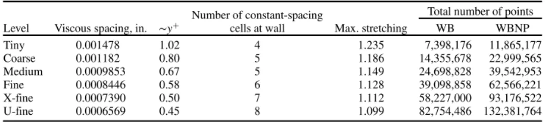
Table 4 CRM WB and WBNP overset grid information
Level Viscous spacing, in. ∼y
Number of constant-spacing
cells at wall Max. stretching
Total number of points
WB WBNP Tiny 0.001478 1.02 4 1.235 7,398,176 11,865,177 Coarse 0.001182 0.80 5 1.186 14,355,678 22,999,565 Medium 0.0009853 0.67 5 1.149 24,698,828 39,542,953 Fine 0.0008446 0.58 6 1.128 39,098,858 62,566,221 X-fine 0.0007390 0.50 7 1.112 58,227,000 93,176,522 U-fine 0.0006569 0.45 8 1.099 82,754,486 132,381,764
for the coarse grid, the zonal grids for the rest of the grid levels were created by running ICEMCFD in batch mode using TCL scripts as previously mentioned. With this approach, the resulting grid system for a given level is made up of a consistent set of zones with the exact same topology applied to the exact same surface definition.
The surface grids were then used to build volume grids using NASA’s Chimera Grid Tools (CGT) package [27] coupled with a NASA TCL script system, which defines boundary conditions for each zone, organizes components with a master configuration file, and drives the CGT programs with a master input file. A script tool called BuildVol generates volume grids where surface grids are run through one of two hyperbolic grid generators (HYPGEN and LEGRID) and Cartesian box grids are created using BOXGR. Grid connectivity was accomplished using PEGASUS5. The resulting system of volume grids is summarized in Table 4. Note that the total number of points shown in this table includes those with an iblank value of 0 (i.e., hole points).
Figure 3 compares surface grid density for the WBNP overset grid family. The WB grids were created by simply removing the NP group and re-running PEGASUS5, and so the grid point clustering on the wing behind the nacelle remained in the WB grid system. This resulted in a consistent set of grids for the NP incremental study.
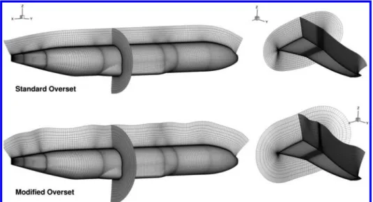
2. UM Modified Overset Grid System
The Standard Overset grid system was generated to provide sufficient overlap of the grids for a node-centered overset solver; however, this overlap was found to be insufficient for the cell-centered ADflow solver. This necessitated a regeneration of the volume meshes to ensure positive volumes, creating a Modified Overset grid system. New volume grids were generated based on the
Fig. 3 CRM WBNP surface grid density variation.
Fig. 4 Modification of nacelle surface mesh.
Fig. 5 Comparison of Standard Overset and Modified Overset body-fitted volume meshes.
field surface meshes of the Standard Overset system. All near-field surface meshes in the Modified Overset system are identical to the Standard Overset meshes, with the exception of the nacelle body grid. It was modified to provide slightly more overlap near the front of the nacelle for coarser meshes. The full mesh refinement series (Tiny through XFine) use this modification, and the number of nodes and spacings are kept consistent with the Standard Overset grids. A comparison of the two Tiny surface meshes are shown in Fig. 4.
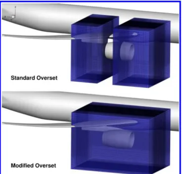
The near-field volume meshes were extruded using an in-house hyperbolic mesh generator. The number of nodes, marching distance, and stretching ratios were kept close to the Standard Overset grids; however, due to the use of a different grid-generation algorithm, the resulting volume meshes differ slightly. A comparison of several slices of the Tiny mesh is depicted in Fig. 5. Finally, the Standard Overset background meshes were used with one exception: the two Cartesian blocks at the leading and trailing edge of the nacelle were merged to create a single block covering the entire nacelle region. This modification is shown in Fig. 6.
An additional, point-matched multiblock mesh was generated for use with the ADflow solver. These grids were generated based on the same meshing guidelines as the Standard and Modified Overset grid systems. A key difference in the grids, as will be highlighted later in Sec. IV, is that the mesh topology in the WB juncture differs. The differences are pictured in Fig. 7. In the overset grid systems, the WB collar grid (Fig. 7a) has all viscous surfaces on the same computational plane. Consequently, there is skew in the grid lines as they extrude outward. In the multiblock system (Fig. 7b), the wing and the body surfaces are separate computational planes, leading to a grid that is more orthogonal.
C. Turbulence Closure
All CFD codes used for the results presented in this work solve the RANS equations, which requires additional closure relations to define the turbulent stress tensor. To this end, all results in this paper were obtained using versions of the one-equation, SA model [10]. This model is rooted in the Boussinesq approximation and uses a field partial differential equation to solve for the eddy viscosity. Additional features/capabilities of the SA model were also employed, such as the Spalart–Shur streamline rotation/curvature correction [11] and a QCR [8]. The use of the rotation/curvature correction, termed the
“SA-RC”variant, improves the model’s prediction around leading edges and in vortex cores. QCR is an extension of the eddy-viscosity
Fig. 6 Revised nacelle–pylon refinement block.
Fig. 7 Grid topology differences in wing-body juncture.
Table 5 Description of solution datasets
ID Dataset name Organization Code
Spatial discretization
Turbulence
model QCR Grid type
q OF-cen2-SARC-noQCR-SO Boeing / NASA OVERFLOW v2.2k Central, O(2) SA-nott2-RC No Standard Overset
r OF-cen2-SARC-QCR-SO Central, O(2) SA-nott2-RC Yes, QCR2000 Standard Overset
o OF-upw3-SARC-QCR-SO Penn State Applied Research Lab OVERFLOW v2.2l Upwind, O(3) SA-noft2-RC Yes, QCR2000 Standard Overset
P OF-weno5-SARC-QCR-SO WENO, O(5) SA-noft2-RC Yes, QCR2000 Standard Overset
a AD-cen2-SA-noQCR-MO University of Michigan ADflow Central, O(2) SA-noft2 No Modified Overset
b AD-cen2-SA-noQCR-MB Central, O(2) SA-noft2 No Multiblock
c AD-cen2-SA-QCR-MB Central, O(2) SA-noft2 Yes Multiblock
e eA-cen2-SA-noQCR-SO ONERA elsA Central, O(2) SA No Standard Overset
f eA-cen2-SA-QCR-S0 Central, O(2) SA Yes, QCR2000 Standard Overset
hypothesis that includes quadratic moments of the strain rate and vorticity tensors to introduce anisotropy to the normal turbulent stresses (u02,v02,w02) that are absent from Boussinesq closures. This
takes the form
τij;QCRτij−CNL1OikτjkOjkτik (1)
where τij is the Boussinesq Reynolds stress tensor based on the SA-model eddy viscosity andOijis a normalized rotation tensor. The value ofCNL1in Eq. (1) is generally set to 0.30 and promotes the
canonical4∶2∶3behavior of the normal stresses in 2D planar shear layers [8]. Use of QCR has been demonstrated to improve solution robustness and accuracy in WB juncture flows, particularly in the presence of incipient separation [9,28].
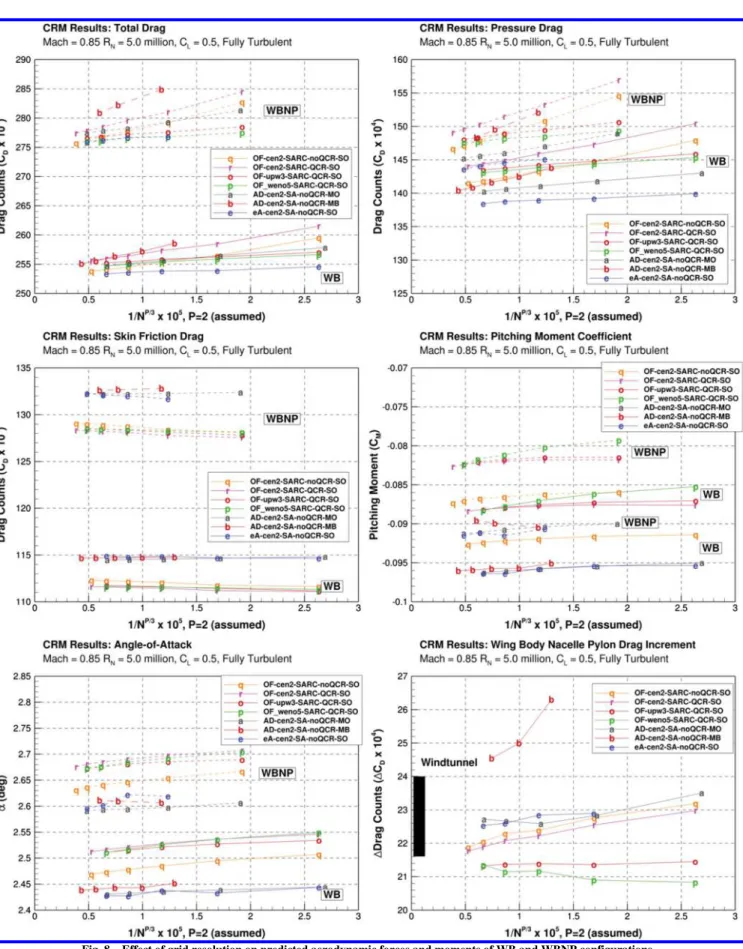
Fig. 8 Effect of grid resolution on predicted aerodynamic forces and moments of WB and WBNP configurations.
IV. Results and Discussion
Various solution strategies and turbulence modeling combinations were employed with the three CFD codes, and these are summarized in Table 5. The ID and Dataset Name are used in subsequent results, and the Dataset Name is formatted as “ Solver-Discretization-TurbulenceModel-QCR-GridSystem.”For example, a second-order central difference solution obtained on the Standard Overset grid system using OVERFLOW with the SARC turbulence model variant and without the QCR option is referred to as “ OF-cen2-SARC-noQCR-SO.”
A. CRM Nacelle–Pylon Drag Increment (Case 2)
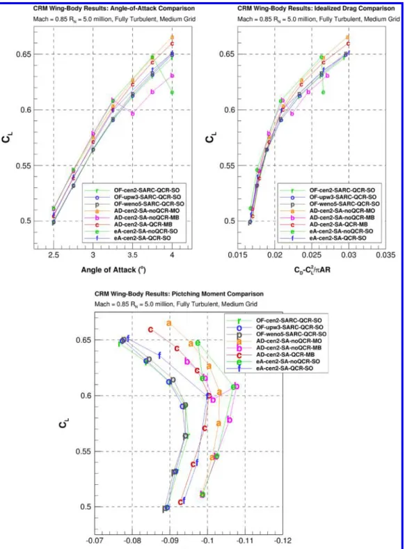
The WB and WBNP grid-convergence study results of all datasets for drag (total, skin friction, pressure, and increment), pitching moment, and angle of attack forCL0.5are plotted in Fig. 8. Total drag values for all solutions are converging to limits between 253 and 255 counts for the WB configuration and between 275 and 277 counts for the WBNP configuration. The predicted NP drag increment for the OVERFLOW solutions is 21–22 counts, whereas ADflow predicts a larger increment of nearly 23 counts. elsA predicts a value just above 22 counts, which is lower than ADflow but higher
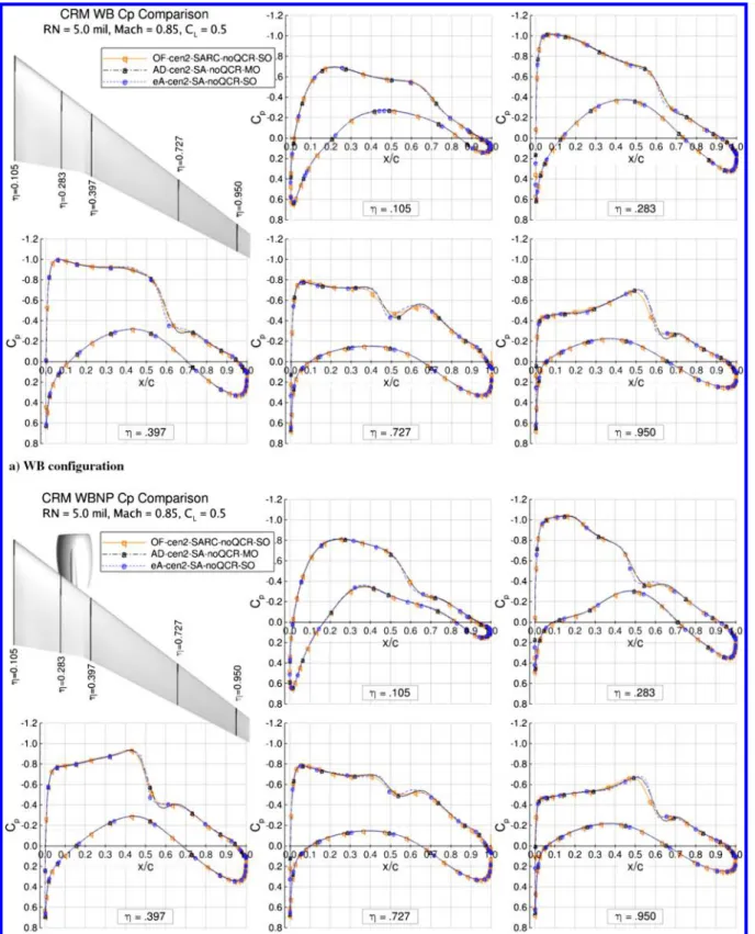
Fig. 9 Predicted surface pressure distributions at select spanwise locations of the WB and WBNP configurations.
than OVERFLOW. Pressure and skin-friction drag components show distinct trends across the solvers. OVERFLOW predicts higher pressure drag than ADflow and elsA for the grid levels considered; however, extrapolating the values to the continuum limit shows the data to be grouped based on whether or not QCR is used. The solutions without QCR predict lower skin-friction drag than those with QCR. Skin-friction drag predictions exhibit two bands: solutions that used OVERFLOW and solutions that did not. Non-OVERFLOW solutions have higher skin-friction drag, and while they did not use QCR, the OVERFLOW values without QCR are more similar to the other OVERFLOW predictions than with the other non-QCR results. Two other factors are also at play between the two groups: the use of the“RC”correction and the solvers being cell-centered versus node-cell-centered.
Predictions for the pitching-moment coefficient are scattered across the various datasets, with the strongest agreement being between the three OVERFLOW solutions with SARC and QCR but with different discretizations. The increase in nose-down moment due to the NP is consistent across all datasets. The angle of attack for
CL0.5exhibits groupings similar to what was observed for the
skin-friction coefficient; however, the OVERFLOW solutions without QCR lies distinctly in between the other OVERFLOW data and the elsA/ADflow data. It may then be inferred that the“RC” correction and QCR alter the angle by approximately 0.05 deg for both the WB and WBNP configurations.
Predicted wing surface pressures for the WB and WBNP configurations are compared in Fig. 9 for all three codes. To provide an appropriate comparison, the plotted solutions represent the use of a second-order central difference scheme without the QCR option. There is very strong agreement between the three codes at all spanwise stations for both configurations. The characteristics of the pressure distributions, including the upper-surface shockwave location, are consistently predicted across the codes. There is some scatter in the details of the shockwave, such as minimum pressure and total pressure rise; however, there appear to be no trends based on the use of the RC correction or the use of standard versus modified overset grids.
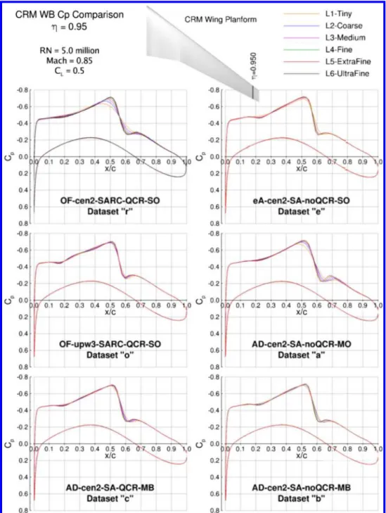
Detailed investigation of the predicted flow fields revealed some inconsistencies across the various solutions in the structure of the shockwave near the tip. An additional weak compression shock
Fig. 10 Surface pressure distributions atη0.95, including the effect of grid resolution and discretization.
appears near the leading edge in this region, giving the shock a lambda-like shape on the surface. A comparison of the pressure distributions at theη0.950station is plotted in Fig. 10 for the solvers at multiple grid refinement levels. For the various central-difference solutions, the location of the primary shockwave does not change as the grid is refined, but the shockwave does sharpen. Refining the grid reveals the presence of a weaker compression around x∕c0.20, upstream of the main shock. The upwinded solution, however, predicts this compression to be stronger and more distinct even for the coarser grid levels. There are numerous possible explanations for the discrepancy in solution behavior, such as upwinding strategy and order of accuracy, and as such, it is the subject of ongoing investigation.
B. CRM WB Static Aero-Elastic Effect (Case 3)
An angle-of-attack sweep ranging from 2.5 to 4.0 deg in quarter-degree increments (7 total angles) was performed using all codes. The grids for each angle of attack were generated based on the measured aeroelastic deformation (bending and twist) from the wind-tunnel tests for the same angles. Polars of the predicted aerodynamic forces and moments are plotted in Fig. 11. As the total drag coefficient includes strong lift-dependent component that obscures solver-specific behaviors, an idealized vortex-induced drag component has been subtracted to provide a pseudo-profile-drag coefficient in the figure.
The various lift curves show distinct banding between the different solution approaches, and this is consistent with the previously
Fig. 11 Aerodynamic characteristics of WB configuration through an alpha sweep.
described behavior for the predicted angle of attack. While the trim cases focused on desired lift coefficient, this study is looking at the behavior at specific angles of attack. All QCR-based solutions show similar lift behavior across the angle-of-attack range, whereas two of the non-QCR datasets exhibit breaks in the lift curve corresponding to the buffet boundary. These breaks in the lift curve correspond with
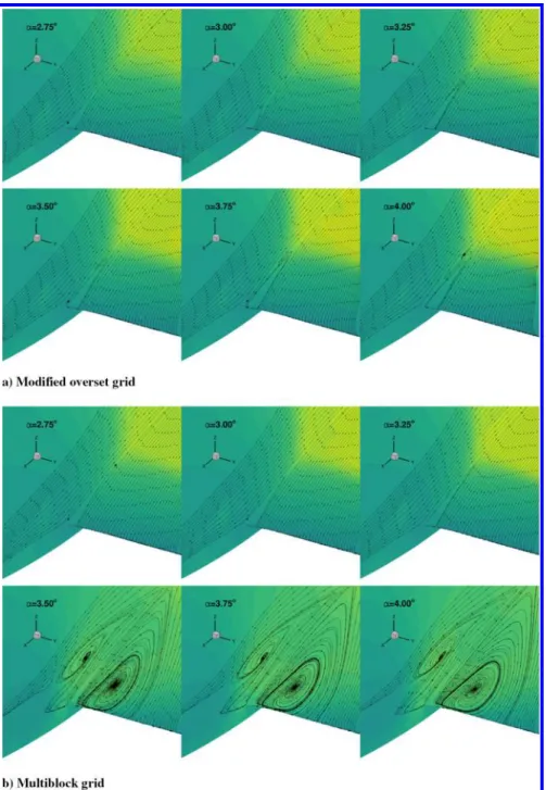
rapid growth of the side-of-body separation bubble in the WB juncture and its interaction with the primary shockwave on the wing. The non-QCR ADflow solutions show a strong dependency on the grid topology. Surface streamlines in the WB juncture for the non-QCR ADflow solutions on both the Modified Overset and Multiblock grid systems are shown in Fig. 12. The solutions on the
Fig. 12 Effect of grid topology on predicted side-of-body separation using ADflow without QCR.
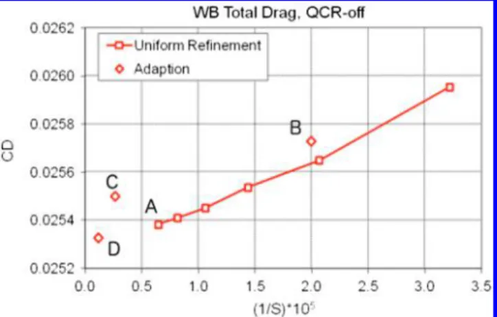
Table 6 OVERFLOW adapted grid parameters Adaption parameters
Case Initial grid Phase Type Region Limit NB levels OB levels Total points Increase WingSrf points Increase
A L6, ufine n/a None n/a n/a n/a n/a 82.8M 156.3K
B L2, coarse n/a None n/a n/a n/a n/a 14.4M 50.3K
C L2, coarse 1 Gradient Wing, wake 100 M 3 2 (wake) 98.3M 6.8× 337.6K 7.7×
D L2, coarse 1 Uniform All zones n/a 1 1
2 Uniform Wing n/a 2 0
3 Gradient Wing, body 400 M 3 2 388.9M 27× 895. IK 17.8×
NB, near-body; OB, off-body.
Existing near-field and far-field box grids were used. Gradient-based adaption used undivided second difference for sensor function.
Modified Overset grid exhibit a smaller bubble and thus no lift break in this angle-of-attack range, whereas the Multiblock solution (with the same surface grids) shows a sharp break between 3.25 and 3.5 deg. The volume grids in this region have differing topologies between the mesh systems, which may be a contributing factor in the drastically different behavior due to the different viscous differencing directions and grid skew. The behavior of the SA model without QCR is known to be inconsistent in juncture flow regions, even for unstructured grids [29], and so the possibility of multiple solutions to the governing equations must be considered.
All of the QCR-based solutions on the Standard Overset meshes (using OVERFLOW and elsA) show strong agreement in the pseudo-profile-drag polar, whereas the QCR-based solutions from ADflow on the multiblock grid exhibit lower drag at the higher angles of
attack. The non-QCR solutions exhibit lower drag values than their QCR counterparts for prebuffet angles of attack. For the pitching-moment coefficient, all QCR-based solutions exhibit less nose-down moment than the non-QCR solutions, and of those, the non-SARC results show greater nose-down moment than the SARC results.
C. CRM WB Grid Adaption (Case 4)
A solution adaption capability for both the Cartesian off-body regions and for curvilinear near-body grids has been implemented in the OVERFLOW overset grid CFD code [30,31]. The adaption capability in OVERFLOW is considered a feature-based process, which does well for hard flow features (e.g., shocks, wakes, and vortices), but is not an output-based or adjoint error-based approach. Building on the Cartesian off-body approach inherent in OVERFLOWand the original adaptive refinement method developed by Meakin [32], the off-body adaption provides for automated creation of multiple levels of finer Cartesian off-body grids. The near-body approach follows closely that used for the Cartesian off-near-body grids, but inserts refined grids in the computational space of original near-body grids. Refined curvilinear grids are generated using parametric cubic interpolation, with one-sided biasing based on curvature and stretching ratio of the original grid. Sensor functions, grid marking, and solution interpolation tasks are implemented in a consistent and efficient way for both the off-body and near-body grids. Refinement is based on normalized second-undivided differences of the flow variables. A goal-oriented procedure, based on largest error first, is included for controlling growth rate and maximum size of the adapted grid system. The adaption process is almost entirely parallelized using MPI, resulting in a capability suitable for viscous, moving body simulations. Coupled with load-balancing and an in-memory solution interpolation procedure, the
Fig. 13 Total drag grid convergence with adaptive results.
Fig. 14 Pressure coefficient comparisons at multiple spanwise wing stations.
adaption process provides very good performance for steady-state and time-accurate simulations on parallel computing platforms.
OVERFLOW’s adaption process was applied to the L2-coarse WB grid defined above. The original L2-coarse grid near body system was modified for use with the adaption process, and the connectivity was switched from a PEGASUS-based approach to the DCF approach (which required the development of a set of XRAYs). All periodic meshes were broken into overlapping grids (OVERFLOW’s adaption cannot be applied to grids with a periodic boundary condition) and the off-body Cartesian boxes were removed. All near-body surface grids were maintained. The total grid size for the new coarse grid is 14.4 million (M) points with 50.3 thousand (K) wing surface points. The new coarse grid case was converged to the same level as the original L2-coarse grid system, labeled Case B below.
Two results from adaption are presented here. In the first case, two levels of near-body adaption were applied to the upper surface of the wing only, along with three levels of off-body adaption (principally to enhance the capture of the wakes and tip vortices). The total number of grid points was restricted to 100 M points, and the resulting adapted grid has 98.3 M total points and 387.6 K wing surface points. Results for this case are labeled C in Table 6. In the second case, first one level of adaption is applied for both the near-body and off-body grids, and then the upper wing grid is uniformly refined two levels to
give a better base for the final three levels of near-body and two levels of off-body grid adaption. This result is labeled“D”in Table 6. The total number of grid points was restricted to 400 M points, and the resulting adapted grid has 388.9 M total points and 895.1 K wing surface points as shown in Table 6. The solution for the L6-ufine grid is used for reference and is labeled“A”below. This grid has 82.8 M points and 156.3 K wing surface points.
Figure 13 shows total computed drag from the adaption cases compared with the grid family results obtained via uniform refinement. The variable (S) plotted along the horizontal axis is the total number of surface grid points. Because this is a 2D evaluation of grid refinement, the powerSis raised to 2/2 instead of 2/3 for 3D. The new coarse grid (DCF mode) result, labeled“B”in Fig. 13, is less than 1 count higher than the original coarse grid (PEGASUS mode) result due to the differences in connectivity and grid topology. The two adaptive cases (C and D) fall to the left of the L6-ufine case (A) due to increased grid count with the adapted case D falling along the asymptotic convergence of grid refinement. Solver convergence was considered good with adaption turned on where multigrid was shut off and 50 iterations were run between adaption cycles.
Figure 14 shows comparisons of theCpat various wing stations, which highlights the improvement in the shock resolution with both increasing grid size and the adaption process. The effect of the
Fig. 15 Effect of adaptation of wing surface grid resolution.
Fig. 16 Effect of adaptation and wing-tip region surface pressure coefficient behavior.
adaption on the shock structure is clearly evident in the adapted cases, especially case D, where the tip shock region shows a well-resolved lambda shape and is more similar to what had been observed in the upwinded MUSCL solution (Fig. 10). The tip region is further explored in Figs. 15 and 16, which show grid resolution and pressure contours for the four cases defined in Table 6. Figure 17 shows a comparison with experimental data [5], with the various cases. The slight compression and expansion at about 20% chord at this station is evident in both the experimental data and the adapted case D.
V. Conclusions
Predictions obtained using the OVERFLOW, elsA, and ADflow structured, overset flow solvers for the 6th AIAA DPW were compared for the NP drag increment and the angle-of-attack sweep. Results were fairly consistent across all solvers, with the prominent differences attributable primarily to the turbulence modeling strategies employed [i.e., SA vs. SARC, quadratic constitutive relation (QCR) vs. non-QCR] and, to a lesser extent, discretization. Some influence of the discretization scheme was observed in the predicted shock structure near the tip. The upwinded MUSCL scheme predicts a more distinct upstream compression compared with the central-difference solutions. Feature-based grid adaption of a central-difference solution responded to this shock, refining the mesh in its vicinity and providing clear resolution of the compression.
Acknowledgments
The authors thank the Boeing Company, ONERA, the National Aeronautics and Space Administration, the Pennsylvania State University Applied Research Laboratory, and the University of Michigan for their support in the Drag Prediction Workshop series.
References
[1] Tinoco, E. N., Brodersen, O., Keye, S., and Laflin, K.,“Summary of Data from the 6th AIAA CFD Drag Prediction Workshop: CRM Cases 2 to 5,”55th AIAA Aerospace Sciences Meeting, AIAA Paper 2017-1208, Jan. 2017.
doi:10.2514/6.2017-1208
[2] Vassberg, J. C., Dehaan, M. A., Rivers, M., and Wahls, R. A., “Development of a Common Research Model for Applied CFD Validation Studies,” 26th AIAA Applied Aerodynamics Conference, AIAA Paper 2008-6919, Aug. 2008.
doi:10.2514/6.2008-6919
[3] Vassberg, J. C., et al.,“Summary of the 4th AIAA Computational Fluid Dynamics Drag Prediction Workshop,”Journal of Aircraft, Vol. 51, No. 4, 2014, pp. 1070–1089.
doi:10.2514/1.C032418
[4] Levy, D. W., et al., “Summary of Data from the 5th AIAA Computational Fluid Dynamics Drag Prediction Workshop,”Journal of
Aircraft, Vol. 51, No. 4, 2014, pp. 1194–1213. doi:10.2514/1.C032389
[5] Rivers, M. B., and Dittberner, A.,“Experimental Investigations of the NASA Common Research Model in the NASA Langley National Transonic Facility and NASA Ames 11-Ft Transonic Wind Tunnel (Invited),”49th AIAA Aerospace Sciences Meeting, AIAA Paper 2011-1126, Jan. 2011.
doi:10.2514/6.2011-1126
[6] Rumsey, C. L., Smith, B. R., and Huang, G. P.,“Description of a Website Resource for Turbulence Modeling Verification and Validation,”40th AIAA Fluid Dynamics Conference and Exhibit, AIAA Paper 2010-4742, June–July 2010.
doi:10.2514/6.2010-4742
[7] Nichols, R. H., and Buning, P. G.,“User’s Manual for OVERFLOW 2.2,”NASA Langley Research Center, Hampton, VA, Aug. 2010. [8] Spalart, P. R.,“Strategies for Turbulence Modelling and Simulation,”
International Journal of Heat and Fluid Flow, Vol. 21, No. 3, 2000, pp. 252–263.
doi:10.1016/S0142-727X(00)00007-2
[9] Sclafani, A. J., Vassberg, J. C., Winkler, C., Dorgan, A. J., Mani, M., Olsen, M. E., and Coder, J. G.,“Analysis of the Common Research Model Using Structured and Unstructured Meshes,”Journal of Aircraft, Vol. 51, No. 4, 2014, pp. 1223–1243.
doi:10.2514/1.C032411
[10] Spalart, P. R., and Allmaras, S. R., “A One-Equation Turbulence Model for Aerodynamic Flows,”Recherche Aerospatiale, No. 1, 1994, pp. 5–21.
[11] Shur, M. L., Strelets, M. K., Travin, A. K., and Spalart, P. R., “Turbulence Modeling in Rotating and Curved Channels: Assessing the Spalart-Shur Correction,” AIAA Journal, Vol. 38, No. 5, 2000, pp. 784–792.
doi:10.2514/2.1058
[12] Jameson, A., Schmidt, W., and Turkel, E.,“Numerical Solution of the Euler Equations by Finite Volume Methods Using Runge Kutta Time Stepping Schemes,” 14th Fluid and Plasma Dynamics Conference, AIAA Paper 1981-1259, 1981.
doi:10.2514/6.1981-1259
[13] Hue, D., Chanzy, Q., and Landier, S.,“DPW-6: Drag Analyses and Increments Using Different Geometries of the CRM Airliner,”Journal of Aircraft, Jan. 2017.
doi:10.2514/1.C034139
[14] Van der Weide, E., Kalitzin, G., Schluter, J., and Alonso, J. J.,“Unsteady Turbomachinery Computations Using Massively Parallel Platforms,” 44th AIAA Aerospace Sciences Meeting, AIAA Paper 2006-0421, Jan. 2006.
doi:10.2514/6.2006-0421
[15] Mader, C. A., Martins, J. R. R. A., Alonso, J. J., and van der Weide, E., “ADjoint: An Approach for the Rapid Development of Discrete Adjoint Solvers,”AIAA Journal, Vol. 46, No. 4, 2008, pp. 863–873.
doi:10.2514/1.29123
[16] Lyu, Z., Kenway, G. K., Paige, C., and Martins, J. R. R. A.,“Automatic Differentiation Adjoint of the Reynolds-Averaged Navier-Stokes Equations with a Turbulence Model,”21st AIAA Computational Fluid Dynamics Conference, AIAA Paper 2013-2581, June 2013.
doi:10.2514/6.2013-2581
[17] Lyu, Z., Kenway, G. K., and Martins, J. R. R. A.,“Aerodynamics Shape Optimization Investigations of the Common Research Model Wing Benchmark,”AIAA Journal, Vol. 53, No. 4, 2015, pp. 968–985. doi:10.2514/1.J053318
[18] Lyu, Z., and Martins, J. R. R. A.,“Aerodynamic Design Optimization Studies of a Blended-Wing-Body Aircraft,”Journal of Aircraft, Vol. 51, No. 5, 2014, pp. 1605–1617.
doi:10.2514/6.1.C032491
[19] Chen, S., Lyu, Z., Kenway, G. K. W., and Martins, J. R. R. A., “Aerodynamic Shape Optimization of the Common Research Model Wing-Body-Tail Configuration,”Journal of Aircraft, Vol. 53, No. 1, 2016, pp. 276–293.
doi:10.2514/1.C033328
[20] Kenway, G. K. W., and Martins, J. R. R. A.,“Multipoint Aerodynamic Shape Optimization Investigations of the Common Research Model Wing,”AIAA Journal, Vol. 54, No. 1, 2016, pp. 113–128.
doi:10.2514/1.J054154
[21] Kenway, G. K. W., Kennedy, G. J., and Martins, J. R. R. A.,“Scalable Parallel Approach for High-Fidelity Steady-State Aeroelastic Analysis and Derivative Computations,”AIAA Journal, Vol. 52, No. 5, 2014, pp. 935–951.
doi:10.2514/1.J052255
[22] Kenway, G. K. W., and Martins, J. R. R. A.,“Multipoint High-Fidelity Aerostructural Optimization of a Transport Aircraft Configuration,” Fig. 17 Comparison at outboard station between experiment[5],
nonadapted, and adapted results.
Journal of Aircraft, Vol. 51, No. 1, 2014, pp. 144–160. doi:10.2514/1.C032150
[23] Landmann, B., and Motagnac, M., “A Highly Automated Parallel Chimera Method for Overset Grids Based on the Implicit Hole Cutting Technique,”Journal for Numerical Methods in Fluids, Vol. 66, No. 6, 2011, pp. 778–804.
doi:10.1002/fld.v66.6
[24] Chan, W. M.,“Enhancements to the Hybrid Mesh Approach to Surface Loads Integration on Overset Structured Grids,”19th AIAA Computa-tional Fluid Dynamics Conference, AIAA Paper 2009-3990, June 2009. doi:10.2514/6.2009-3990
[25] “ANSYS ICEM CFD 15.0,”ANSYS, Inc., Canonsburg, PA, Nov. 2013. [26] Vassberg, J. C., DeHaan, M. A., and Sclafani, A. J.,“Grid Generation Requirements for Accurate Drag Predictions Based on OVERFLOW Calculations,”16th AIAA Computational Fluid Dynamics Conference, AIAA Paper 2003-4124, June 2003.
doi:10.2514/6.2003-4124
[27] Chan, W. M., Rogers, S. E., Pandya, S. A., Kao, D. L., Buning, P. G., Meakin, R. L., Boger, D. A., and Nash, S. M.,“Chimera Grid Tools User’s Manual, Version 2.1,”NASA Ames Research Center, Moffett Field, CA, 2010.
[28] Yamamoto, K., Tanaka, K., and Murayama, M.,“Effect of a Nonlinear Constitutive Relation for Turbulence Modeling on Predicting Flow
Separation at Wing-Body Juncture of Transonic Commercial Aircraft,” 30th AIAA Applied Aerodynamics Conference, AIAA Paper 2012-2895, June 2012.
doi:10.2514/6.2012-2895
[29] Park, M. A., Laflin, K. R., Chaffin, M. S., Powell, N., and Levy, D. W., “CFL3D, FUN3D, and NSU3D Contributions to the 5th Drag Prediction Workshop,” Journal of Aircraft, Vol. 51, No. 4, 2014, pp. 1268–1283.
doi:10.2514/1.C032613
[30] Buning, P. G., and Pulliam, T. H.,“Cartesian Off-Body Grid Adaption for Viscous Time-Accurate Flow Simulations,”20th AIAA Computa-tional Fluid Dynamics Conference, AIAA Paper 2011-3693, June 2011. doi:10.2514/6.2011-3693
[31] Buning, P. G., and Pulliam, T. H.,“Near-Body Grid Adaption for Overset Grids,” 46th AIAA Fluid Dynamics Conference, AIAA Paper 2016-3326, June 2016.
doi:10.2514/6.2016-3326
[32] Meakin, R. L.,“An Efficient Means of Adaptive Refinement within Systems of Overset Grids,”12th AIAA Computational Fluid Dynamics Conference, AIAA Paper 1995-1722, June 1995.
doi:10.2514/6.1995-1722
![Table 1 CRM wing geometric reference parameters [2]](https://thumb-us.123doks.com/thumbv2/123dok_us/275179.2528284/2.877.89.388.169.643/table-crm-wing-geometric-reference-parameters.webp)