The Variable-Rate Decision for Multiple Inputs with Multiple Management Zones

The Variable-Rate Decision for Multiple Inputs with Multiple Management Zones

Roland K. Roberts, Burton C. English, and James A. Larson Department of Agricultural Economics, University of Tennessee

2126 Morgan Circle, Knoxville, TN 37996-4518 [email protected], (865) 974-7482

Selected Paper Prepared for Presentation at the

Southern Agricultural Economics Association Annual Meeting Little Rock, Arkansas, February 5-9, 2005

Abstract: Research has evaluated the relative profitability of variable-rate versus uniform-rate application of a single input in fields with multiple management zones. This paper addresses the variable-rate decision for multiple inputs. The decision-making framework is evaluated for nitrogen and water applied to irrigated cotton in fields with three management zones.

Keywords: Breakeven analysis, cotton, economic feasibility, multiple inputs, precision farming, variable-rate technology

JEL Classifications: Q12

Copyright 2005 by Roland K. Roberts, Burton C. English, and James A. Larson. All rights reserved. Readers may make verbatim copies of this document for non-commercial purposes by any means, provided that this copyright notice appears on all such copies.

The Variable-Rate Decision for Multiple Inputs with Multiple Management Zones Introduction

Economic analyses of the decision to use variable-rate technology (VRT) versus uniform-rate technology (URT) to apply inputs within a farm field have concentuniform-rated on application of a single input (eg., Lambert and Lowenberg-DeBoer; Swinton and Lowenberg-DeBoer; English, Roberts, and Mahajanashetti). Unless inputs are independent of one another, a change in the quantity of one input affects the marginal product of the other inputs as they interact in

producing output. Thus, for the multiple input VRT decision, the optimal quantities of the inputs for each management zone must be determined by the simultaneous solution of the first order conditions for profit maximization. This paper considers the profit-maximizing decision about whether to use VRT or URT to apply multiple inputs within a field and evaluates this decision for cases where nitrogen and water are applied to cotton fields with different proportions of their acreage in three management zones.

Farmers are interested in knowing whether VRT is economically viable for their fields. Profitability of VRT varies across fields with differences in spatial variability, where spatial variability is defined as the distribution across a field of management zones with different crop yield responses to inputs (Roberts, English, and Mahajanashetti). Within-field variability in soil physical and chemical characteristics is a necessary condition for the economic viability of using VRT (English, Roberts, and Mahajanashetti; Forcella; Hayes, Overton, and Price; Roberts, English, and Mahajanashetti; Snyder). Relationships among crop yields, input levels, and soil characteristics determine spatial variability within a field. These relationships also determine yield response variability, where yield response variability is defined as the differences in magnitudes of yield response among management zones (English, Roberts, and Mahajanashetti;

Forcella; Roberts, English, and Mahajanashetti). Spatial and yield response variability, along with the crop price, the input prices, and the additional cost of using VRT versus URT, in concert with farmer and farm characteristics, factor into the decision to adopt VRT (Roberts et al., 2004). In the end, no general formula exists for determining whether VRT or URT should be used on a particular field because each field presents a different case (Roberts et al., 2002).

The objectives of this paper are to 1) present an analytical framework for the VRT versus URT decision for applying multiple inputs in fields with multiple management zones and 2) illustrate the decision-making framework for irrigated cotton fields with nitrogen and water applied to three management zones.

Analytical Framework

Assume farmers are profit maximizers who can classify their fields into m management zones and have knowledge of the management-zone-specific yield response functions for a given crop and set of n inputs. Suppose further that yield responses can be represented by concave functions and fields can include any of these m management zones in any proportions. Let the response functions be represented by equations (1).

(1) Yi = Yi (Xi1,…,Xin) i = 1,2,…,m

where Yi is crop yield/acre for management zone i and Xij is the amount of input j (j=1,…,n) applied per acre to management zone i.

Economically optimal quantities of the n inputs are determined for a particular

management zone by equating the marginal physical products of the yield response function for that management zone with the input-to-crop price ratios and solving these equations

simultaneously for input quantities. These n equations are the first order conditions for profit maximization for that management zone. Optimal quantities of inputs are different for each

management zone. Optimal return above input costs per acre for the field under VRT ( ) is then calculated from the following profit function (Nicholson):

* VRT R (2) * = [ Y VRT R

∑

= λ m 1 i i Y P i (Xi1 *,…, Xin *) – ij* n 1 j jX P

∑

= ] = * ( , , ) VRT R λ₁,λ₂,...,λ_m−1 P_Y P₁,...,P_n

where P_Y is the crop price; is the price of input j (j=1,…,n); XP_j ij * is the optimal input

(j=1,…n) application rate for the ith management zone; is optimal net return above input costs for the i

* i

π

th _{management zone; and is the proportion of the field in the i}

i

λ th _{management zone}

such that

∑

= 1. Thus, is the weighted average over =

λ

m 1 i

i R*VRT λi of the optimal returns above

input costs per acre obtained for each management zone. The proportion of the field in management zone m (λ_m) is not included as an argument in the * function because

VRT R λ_m = 1 –

∑

− . = λ 1 m 1 i i

Numerous decision rules could be assumed for URT application of the inputs (English, Roberts, Majajanashetti). In this paper, farmers are assumed to base URT decisions on the profit-maximizing input levels obtained from a field-average yield response function, with the proportions of the field in each management zone ( ) serving as weights. Determining the optimal uniform rate based on the weighted average response function is analogous to some methods used to develop fertilizer recommendations. For example, receiving a recommendation from a soil-test laboratory based on a soil sample that mixes soil cores drawn at random across a field (VanEck and Collier) is similar to weighting the recommendations for the management zones by the proportions of the field in each management zone. In addition, soil-test laboratories

s

and the Extension Service often base their fertilizer recommendations on yield goals developed by farmers (Savoy and Joines). These yield goals can be formed in a variety of ways (O’Neal et al.). If the farmer forms the field yield goal by implicitly averaging yield goals across

management zones, the field yield goal and the fertilizer recommendation would be weighted by the proportions of the field in each management zone.

Assume the farmer determines optimal uniform application rates based on the field-average response function expressed as:

(3) Yu = Yu (Xu1 ,…, Xun ) =

∑

Y = λ m 1 i i i (Xu1 ,…, Xun)

where Yu is the weighted average crop yield response function for the field and Xuj is the uniform application rate for input j (j=1,…,n). The optimal return above input cost per acre for URT ( * ) is calculated from the following profit function:

URT R (4) * = Y URT R P_Y

∑

= λ m 1 i i i (Xu1 *_{,…, X} un*) – uj* n 1 j jX P

∑

= = * ( , , ) URT R λ1,λ2,...,λm−1 PY P1,...,Pn

where Xuj* is the optimal uniform application rate for input j obtained from the field-average yield response function through the simultaneous solution of the n first order conditions for profit maximization, which equate the marginal products of the inputs with their respective input-to-crop price ratios. Again λ_m is excluded as an argument because the sum of the s equals 1. λ_i

The difference between * and , which is the optimal return to VRT (RVRT

VRT

R *

URT

R *),

can be specified as:

(5) RVRT* = * - = RVRT

VRT

R *

URT

R *(λ₁,λ₂,...,λ_m−1, P_Y, P₁,...,P_n) where all variables have been previously defined.

VRT is more profitable than URT if RVRT* – V₁– V₂ > 0, where is the application cost for VRT minus the application cost for URT and is the cost of gathering spatial

information and using it to identify management zones and their yield response functions. If the management zones and their response functions have already been identified, is known and the farmer will undertake VRT if RVRT

1 V 2 V 2 V

* _{> , because is a sunk cost in making the VRT}

versus URT decision. If, on the other hand, is not known, the farmer can use conservative, educated guesses about the s, the corresponding yield response functions, and to estimate RVRT 1 V V₂ 2 V i λ V₁

* _{– , which can be thought of as an education guess about the maximum amount a}

farmer can invest in gathering spatial information and identifying the field’s management zones and their yield response functions.

1

V

Equation (5) is concave in . Its concavity can easily be understood by considering fields with three management zones; management zones 1, 2, and 3. For fields that are all in management zone 1 ( = 1, = 0, and = 0), RVRT

i

λ

1

λ λ₂ λ₃ * = 0 because the weighted average response function and the response function for management zone 1 are the same. Fields with a positive and/or (0 < <1) have multiple management zones and farmers can consider using VRT. Since optimization of input use with VRT is more suited to the site-specific yield response functions than to the field-average response function, RVRT

2

λ λ₃ λ₁

* _{now becomes positive}

and continues to increase to a maximum as decreases over some range. λ₁

Spatial Break-even Variability Proportions (SBVPs) (English, Roberts, and

Mahajanashetti; Mahajanashetti; Roberts, English, and Mahajanashetti) are defined as the lower and upper limits of λ_m−2, λ_m−1, and λ_m for given levels of λ₁,λ₂,...,λ_m−3, P_Y, , and VP_j 1 such

that RVRT* = V1, where V1 is the additional application cost of using VRT compared to URT. Mathematically, equation (5) can be modified as follows and used to locate the SBVPs for λ_m−2,

, and .

1 m−

λ λ_m

(6) RVRT* = RVRT*(λ_m−1,λ_m−2⏐λ₁,λ₂,...,λ_m−3, P , _Y P₁,...,P_n) = V ₁

where λ₁,λ₂,...,λ_m−2, P , _Y P (j=1,…,n), and _j V are given levels of the respective variables and ₁

= 1 – – m λ λ_m−2 −λ_m−1

∑

− = 3 m 1 i i. λ

As a more specific example using a concave functional form, assume three management zones and express equations (1) as quadratic yield response functions containing two inputs with interaction between the inputs. Given these assumptions, the functional forms of equations (2), (4), and (5) can be determined and the SBVPs can be identified. Let the respective management-zone proportions be , , and , and let equations (1) be represented by equations (7), (8), and (9). 1 λ λ₂ λ₃ (7) 2 _{1 11 12} 12 1 12 1 2 11 1 11 1 1 1 a b X c X d X e X f X X Y = + + + + + (8) 2 _{2 21 22} 22 2 22 2 2 21 2 21 2 2 2 a b X c X d X e X f X X Y = + + + + + (9) 2 _{3 31 32} 32 3 32 3 2 31 3 31 3 3 3 a b X c X d X e X f X X Y = + + + + +

where Yi and Xij are defined in equations (1) for m = 3 management zones (i=1, 2, and 3) and n = 2 inputs (j=1 and 2).

For VRT, take the partial derivative of the yield response function for management zone I with respect to inputs 1 and 2, set these derivatives equal to the price of input j divided by the price of the output, and solve the two equation simultaneously (Heady and Dillon) for X*i1 and X*

(10) X

[

(

( ) (

Pf 2d P

)

/P

)

(2bd cf )

]

/(f2 4c_ie_i) i i i i i y 1 i i 2 * i1 = + − + − (11) X

[

(

( ) (

Pf 2c P

)

/P

)

(2cd bf )

]

/(f2 4c_ie_i) i i i i i y 2 i i 1 * 2i = + − + −

Substitute these optimal input rates into equations (7, 8, and 9), substitute the resulting optimal yields into equation (2) to determine the net return for management zone i, do the same for each management zone, and weight these net returns based on to get . For URT, substitute equations (7), (8), and (9) into equation (3) and set X

i

λ *

VRT

R

1j = X2j = X3j = Xuj (j=1 and 2). Set the derivative of the resulting field-average yield response function equal to / and solve for X

j

P PY

uj*. Substitute these optimal uniform input application rates into equation (3) and substitute the resulting optimal field-average yield into equation (4) to get . Calculation of RVRT* is straight forward from equation (5).

* URT

R

Illustrative Example

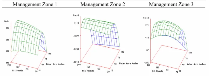
To illustrate the concepts presented above, assume hypothetical fields suited to cotton production can be classified into three management zones and that the following quadratic functions represent cotton yield response to fertilizer nitrogen and irrigation plus initial moisture (W) for the management zones.

(12) 2 _{1 1} 1 1 2 1 1 1 233.72 23.65*W 0.182*W 0.439*N 0.0033*N 0.021*W *N Y = + − + − + (13) Y₂ =−1103.6+118.35*W₂ −1.63*W₂2 +2.85*N₂ −0.004*N₂2 −0.046*W₂*N₂ (14) Y₃ =−170.93+32.45*W₃−0.022*W₃2 +3.74*N₃ −0.011*N₃2 +0.022*W₃*N₃ where Y1, Y2, and Y3 are cotton lint yields (lb/acre); W1, W2, and W3 are the amounts of water applied plus 5 inches of available preplant moisture plus 1 inch of rainfall (acre-inches); N1, N2, and N3 are nitrogen application rates (lb/acre); and the subscripts represent the three management

zones. These equations were estimated by Hexem and Heady in the mid 1970’s using field data. They were estimated as quadratic yield response functions similar to those in Arce-Diaz et al., Agrawal and Heady, Mjelde et al., Vanotti and Bundy, and Schlegel and Havlin. These functions would be somewhat different if estimated with current data. Nevertheless, they are plausible irrigated cotton yield response functions, chosen for illustrative purposes to serve as examples in this paper. Their use facilitates exposition of the aforementioned concepts because they are continuous and concave. The response functions are portrayed graphically in Figure 1. An average cotton lint price received by farmers (P =$0.52/lb) and an average nitrogen _Y price (PN=$0.26/lb) over the 2000-2003 period and an irrigation water price of $4.00/acre-inch

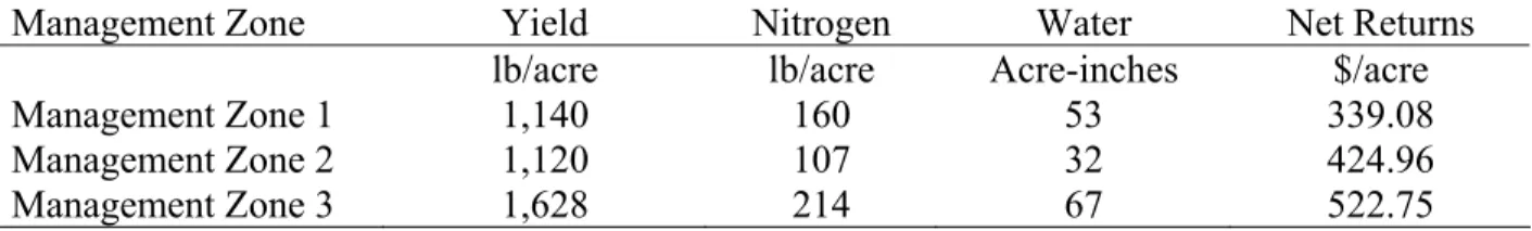
were used in the analysis. Optimal yields, input application rates, and net returns above input costs were determined for each management zone (Table 1). was determined as a

weighted average of the last column in Table 1, given the assumptions about the . was calculated using the field-average yield response function to determine optimal field-average input application rates, corresponding yields, and net returns above input costs for each management zone, weighted by the assumed . In this example, RVRT* was evaluated for hypothetical cotton fields for all combinations of the when each λ varied between 0.0 and 0.9 in increments of 0.1 (eg., = 0.0, = 0.4, and = 0.6 or

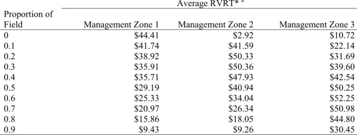
* VRT R s λ_i * URT R s λ_i s λ_i 1 λ λ₂ λ₃ λ₁= 0.2, λ₂= 0.5, and λ₃= 0.3). For illustrative purposes, Table 2 presents average RVRT*s for all combinations of two assuming the for one management zone is fixed at the level in the first column. For example, if the proportion of the field in management zone 1 is fixed at the average RVRT s λ_i λ , 0 . 0 λ₁ =

* _{is $44.41/acre for fields with all combinations of and between 0.0 and 0.9.}

2

Average RVRT* declines as the proportion of land in management zone 1 increases. Management zone 1 is the least profitable management zone and increasing its proportion relative to the other two management zones decreases expected profit and impacts RVRT*. If management zone 2 is either non-existent or makes up 90% of the field, RVRT* is less than $10/acre. The highest RVRT* for management zone 2 is reached when it constitutes between 20 and 30% of the field. The highest RVRT* for management zone 3 is reached when the field has about 60% of its area in this management zone.

The additional charge for VRT versus URT application of inputs can be separated into two componentsV₁ = V_1N +V_1W, where V_1N is the difference between the cost of VRT versus URT application of nitrogen and V_1W is the difference between the cost of VRT versus URT application of irrigation water. The additional custom charge for variable-rate nitrogen application compared to uniform-rate application was assumed to beV_1N = $3.00/acre. This additional charge was close to the mean of $3.08/ac (range $1.50 to $5.50/acre) obtained from personal telephone interviews with firms providing precision farming services to Tennessee farmers (Roberts, English, and Sleigh). Responding firms indicated that the additional charge would include the difference in application costs for VRT versus URT and a charge to create a nitrogen application map based on soil survey maps in conjunction with the consultant’s

knowledge about corn response on various soils, a visit to the field to observe conditions, and an interview with the farmer about historical yields. Based on information developed in Georgia (Fairchild), a center pivot system can be retrofitted for somewhere in the $5,000-to-$10,000 range depending on the number of sprinklers controlled. Assuming a 5-year life, no salvage value and a 150-acre irrigation system, the additional cost is $9 to $18/acre. Therefore, a farmer

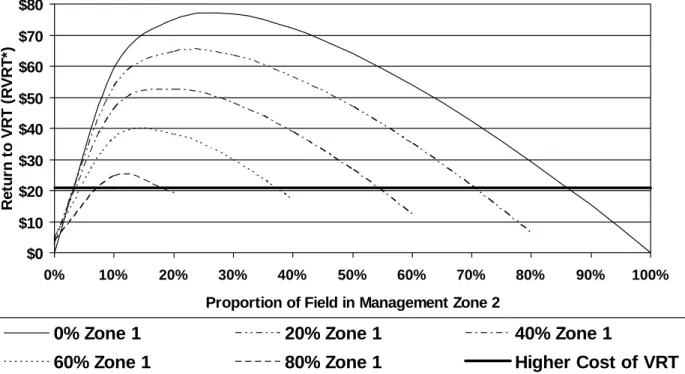
would have to receive an RVRT* of between $12 and $21/acre to break even with URT application of these two inputs. This increase in net returns would have to come from either increased yields and/or decreased input usage compared to URT application of nitrogen and water.

If the field has no area in management zone 1 (Figure 2), management zone 2 must be greater than 4% or less than 90% of the field for VRT application of nitrogen and water to provide equal or higher net returns than URT application and management zone 3 has to be between 96% (100% – 4%) and 10% (100% – 90%) of the field because management zones 2 and 3 comprise 100% of the field. If the field is 30% management zone 2 and 0% management zone 1, the expected net return to VRT is $77/acre (RVRT*) minus $21/acre (V ) or $56/acre. ₁ As the percentage of a field in management zone 1 increases, the SBVP’s become narrower. If the proportion of management zone 1 is 60%, the SBVPs for management zone 2 (management zone 3) are 7.5% (32.5% = 100% – 60% – 7.5%) and 38% (2% = 100% – 60% – 38%). Within these ranges of λ₂ and λ₃ (given = 0.6), RVRT* – λ₁ V is greater than or equal to zero and the ₁ farmer at least breaks even by using VRT.

Conclusions

The extent that multiple-input VRT is adopted will depend on the expected net economic benefits received by potential adopters. Fields generally exhibit yield variability; however, as demonstrated in this paper, not all fields warrant VRT from an economic standpoint. Farmers are interested in knowing whether VRT is economically viable on their fields. The answer to this question varies from field to field depending on spatial variability as well as yield response variability among management zones. The answer also varies with the crop, the inputs, their prices, and the cost of using VRT relative to URT. In the end, no general formula exists for

determining whether VRT or URT should be used on a particular field because each field presents a different case. Nevertheless, for the case presented in this paper, a wide range of spatial variability would provide increased net returns for VRT application of nitrogen and water relative to URT application.

To utilize this methodology, farmers need knowledge of the field-specific management zones for a particular crop and inputs, including the parameters of the corresponding yield response functions. Unfortunately, this knowledge is difficult to obtain with certainty, but farmers are currently using other precision farming technologies (eg., yield monitors, grid soil sampling, field mapping) that can be used to identify management zones and their yield response potentials (English, Roberts, and Sleigh). Even when information about the management zones and yield response functions is not known, these methods can be used to obtain rough estimates about whether investment in obtaining additional spatial information to more precisely identify management zones and estimate their corresponding yield response functions is potentially worthwhile.

References

Agrawal, R.C. and E.O. Heady. Operations Research Methods for Agricultural Decisions. Ames, IA: Iowa State University Press, 1972.

Arce-Diaz, E., A.M. Featherstone, J.R. Williams, and D.L. Tanaka. “Substitutability of Fertilizer and Rainfall for Erosion in Spring Wheat Production.” Journal of Production Agriculture 6(1993):72-76.

English, B.C., R.K. Roberts, and S.B. Mahajanashetti. “Assessing Spatial Break-Even Variability in Fields with Two or More Management Zones.” Journal of Agricultural and Applied Economics 33(2001):551-565.

English, B.C., R.K. Roberts, and D.E. Sleigh. “Spatial Distribution of Precision Farming Technologies in Tennessee.” Tennessee Agricultural Experiment Station, Department of Agricultural Economics, Research Report 00-05, 2000.

Fairchild, B. “Water in the Right Spot.” AgWeb.com. Available on line at:

http://www.farmjournal.com/pub_get_article.asp?sigcat=&pageid=96373. Published March 22, 2003 (accessed December 30, 2004).

Forcella, F. “Value of Managing Within-Field Variability.” pp. 125-132. In (P.C. Robert, R.H. Rust, and W.E. Larson, eds.) Proceedings of the First Workshop on Soil-Specific Crop Management: A Workshop on Research and Development Issues. American Society of Agronomy, Crop Science Society of America, Soil Science Society of America, Madison, WI, 1992.

Hayes, J.C., A. Overton, and J.W. Price. “Feasibility of Site-Specific Nutrient and Pesticide Applications.” In (K.L. Campbell, W.D. Graham, and A. B. Bottcher, eds.) Proceedings of the Second Conference on Environmentally Sound Agriculture. Orlando, FL, April 20-22, 1994. St. Joseph, MI: American Society of Agricultural Engineers, 1994:62–68.

Heady, E.O., and J. L. Dillion. Agricultural Production Functions. Ames, IA: Iowa State University Press, 1972.

Hexem, R., and E.O. Heady. Water Production Functions for Irrigated Agriculture. Ames, IA: Iowa State University Press, 1978.

Lambert, D., and Lowenberg-DeBoer. “Precision Agriculture Profitability Review.” Site-Specific Management Center. West Lafayette, IN: Purdue University. Available online at: http://www.purdue.edu/ssmc. Published September 15, 2000 (accessed January 13, 2005). Mahajanashetti, S.B. “Precision Farming: An Economic and Environmental Analysis of

Mjelde, J.W., J.T. Cothren, M.E. Rister, F.M. Hons, C.G. Coffman, C.R. Shumway, and R.G. Lemon. “Integrating Data from Various Field Experiments: The Case of Corn in Texas.” Journal of Production Agriculture 4(1991):139-147.

Nicholson, W. Microeconomic Theory: Basic Principles and Extensions, 9th ed. Mason, Ohio: South-Western/Thomson Learning, 2004.

O’Neal, M.R., J.R. Frankenberger, D.R. Ess, and J.M. Lowenberg-DeBoer. “Impact of Spatial Precipitation Variability on Profitability of Site-Specific Nitrogen Management Based on Crop Simulation.” Paper No. 001014 presented at the 2000 ASAE Annual International Meeting, Milwaukee, WI, July 8-12, 2000.

Roberts, R.K., B.C. English, and S.B. Mahajanashetti. “Evaluating the Returns to Variable Rate Nitrogen Application.” Journal of Agricultural and Applied Economics 32(2000):133-143. Roberts, R.K., B.C. English, and D.E. Sleigh. “Precision Farming Services in Tennessee Results

of a 1999 Survey of Precision Farming Service Providers.” Tennessee Agricultural

Experiment Station, Department of Agricultural Economics, Research Report 00-06, 2000. Roberts, R.K., B.C. English, J.A. Larson, R.L. Cochran, W.R. Goodman, S.L. Larkin, M.C.

Marra, S.W. Martin, W.D. Shurley, and J.M. Reeves. “Adoption of Site-Specific Information and Variable Rate Technologies in Cotton Precision Farming.” Journal of Agricultural and Applied Economics 36(2004):143-158.

Roberts, R.K., S.B. Mahajanashetti, B.C. English, J.A. Larson, and D.D. Tyler. “Variable Rate Nitrogen Application on Corn Fields: The Role of Spatial Variability and Weather.” Journal of Agricultural and Applied Economics 34(2002):111-129.

Savoy, H.J., Jr., and D. Joines. “Lime and Fertilizer Recommendations for the Various Crops of Tennessee.” The University of Tennessee Institute of Agriculture, Agricultural Extension Service, P&SS Info No. 185, 1998.

Schlegel, A.J. and J.L. Havlin. “Crop Response to Long-term Nitrogen and Phosphorous Fertilization.” Journal of Production Agriculture 8(1995):181-185.

Snyder, C.J. “An Economic Analysis of Variable-Rate Nitrogen Management Using Precision Farming Methods.” Ph.D. Dissertation. Kansas State University, 1996.

Swinton, S.M., and J. Lowenberg-DeBoer. “Evaluating the Profitability of Site-Specific Farming.” Journal of Production Agriculture 11(1998):439-446.

VanEck, W.A., and C.W. Collier, Jr. “Sampling Soils.” West Virginia University Extension Service. Available on line at: http://www.caf.wvu.edu/~forage/3201.htm. Published September 1995 (Accessed January 13, 2005).

Vanotti, M.B. and L.G. Bundy. “An Alternative Rationale for Corn Nitrogen Fertilizer Recommendations.” Journal of Production Agriculture 7(1994):243-249.

Table 1. Optimal Yields, Input Application Rates, and Net Returns above Input Costs for Management Zones 1 through 3

Management Zone Yield Nitrogen Water Net Returns

lb/acre lb/acre Acre-inches $/acre

Management Zone 1 1,140 160 53 339.08

Management Zone 2 1,120 107 32 424.96

Table 2. Average Returns to Variable-Rate Application of Nitrogen and Water (RVRT*) for Selected Management Zone Proportions

Average RVRT* a

Proportion of

Field Management Zone 1 Management Zone 2 Management Zone 3

0 $44.41 $2.92 $10.72 0.1 $41.74 $41.59 $22.14 0.2 $38.92 $50.33 $31.69 0.3 $35.91 $50.36 $39.60 0.4 $35.71 $47.93 $42.54 0.5 $29.19 $40.94 $50.25 0.6 $25.33 $34.04 $52.25 0.7 $20.97 $26.34 $50.98 0.8 $15.86 $18.05 $44.80 0.9 $9.43 $9.26 $30.45

a _{Average RVRT*, represented by the fixed in the first column and the management zone in} the column, is determined by averaging the RVRT*s for fields with all combinations of the other two s. For instance, the $9.43/acre return in the column headed Management Zone 1 is the average return when the field is 90% management zone 1 and either 10% management zone 2 ($16.38/acre) or 10% management zone 3 ($2.37/acre).

λ λ

Management Zone 1 Management Zone 2 Management Zone 3

Figure 1. Graphical Portrayal of the Cotton Yield Response Functions Used in the Analysis

$0 $10 $20 $30 $40 $50 $60 $70 $80 0% 10% 20% 30% 40% 50% 60% 70% 80% 90% 100%

Proportion of Field in Management Zone 2

R e tu rn to V R T (R V R T *)

0% Zone 1 20% Zone 1 40% Zone 1

60% Zone 1 80% Zone 1 Higher Cost of VRT

Figure 2. Spatial Breakeven Variability Proportions for Management Zones 2 and 3 Given a Predetermined Proportion for Management Zone 1