E
XCEL
M
ODELING AND
E
STIMATION
IN
I
NVESTMENTS
Third
Edition
CRAIG W. HOLDEN
Max Barney Faculty Fellow and Associate Professor Kelley School of Business
Indiana University
CONTENTS
Preface ... vii
Third Edition Changes ... vii
What Is Unique About This Book ... x
Conventions Used In This Book ... xii
Craig’s Challenge ... xiii
The Excel Modeling and Estimation Series ... xiii
Suggestions for Faculty Members ... xiv
Acknowledgements ... xv
About The Author ... xvi
PART 1 BONDS / FIXED INCOME
SECURITIES ... 1
Chapter 1 Bond Pricing ... 1
1.1 Annual Payments ... 1
1.2 EAR and APR ... 2
1.3 By Yield To Maturity ... 3
1.4 Dynamic Chart... 4
1.5 System of Five Bond Variables ... 5
Problems ... 6
Chapter 2 Bond Duration ... 8
2.1 Basics ... 8
2.2 Price Sensitivity using Duration ... 10
2.3 Dynamic Chart... 12
Problems ... 14
Chapter 3 Bond Convexity ... 15
3.1 Basics ... 15
3.2 Price Sensitivity Including Convexity ... 16
3.3 Dynamic Chart... 19
Problems ... 21
Chapter 4 The Yield Curve ... 22
4.1 Obtaining It From Treasury Bills and Strips ... 22
4.2 Using It To Price A Coupon Bond ... 23
4.3 Using It To Determine Forward Rates ... 25
Problems ... 25
Chapter 5 US Yield Curve Dynamics ... 27
5.1 Dynamic Chart... 27
Problems ... 33
Chapter 6 Affine Yield Curve Models ... 35
6.1 The Vasicek Model ... 35
6.2 The Cox-Ingersoll-Ross Model ... 38
PART 2 STOCKS / SECURITY
ANALYSIS ... 41
Chapter 7 Portfolio Optimization ... 41
7.1 Two Risky Assets and a Riskfree Asset ... 41
7.2 Descriptive Statistics ... 44
7.3 Many Risky Assets and a Riskfree Asset ... 49
Problems ... 60
Chapter 8 Constrained Portfolio Optimization ... 62
8.1 No Short Sales, No Borrowing, and Other Constraints ... 62
Problems ... 78
Chapter 9 Asset Pricing ... 79
9.1 Static CAPM Using Fama-MacBeth Method ... 79
9.2 APT or Intertemporal CAPM Using Fama-McBeth Method ... 84
Problems ... 91
Chapter 10 Trading Simulations using @RISK ... 93
10.1 Trader Simulation ... 93
10.2 Dealer Simulation ... 109
Chapter 11 Portfolio Diversification Lowers Risk ...127
11.1 Basics ... 127
11.2 International ... 129
Problems ... 131
Chapter 12 Life-Cycle Financial Planning ...132
12.1 Basics ... 132
12.2 Full-Scale Estimation ... 134
Problems ... 142
Chapter 13 Dividend Discount Models ...143
13.1 Dividend Discount Model ... 143
Problems ... 144
Chapter 14 Du Pont System Of Ratio Analysis ...145
14.1 Basics ... 145
Problems ... 146
PART 3 OPTIONS / FUTURES /
DERIVATIVES ... 147
Chapter 15 Option Payoffs and Profits ...147
15.1 Basics ... 147
Problems ... 149
Chapter 16 Option Trading Strategies ...150
16.1 Two Assets ... 150
16.2 Four Assets ... 155
Problems ... 159
Chapter 17 Put-Call Parity ...162
17.1 Basics ... 162
17.2 Payoff Diagram ... 162
Chapter
18. 18. 18.3 18. 18. 18. ProChapter
19. 19. 19.3 19. 19. ProChapter
20. 20. ProChapter
21. 21. ProChapter
22. 22. ProPART
Chapter
23. 23. 23.3 23. 23. 23. 23. 23. 23. 23. 23.C
ONTE
Re Ex Ch Ch Chr 18 Binom
1 Estimating 2 Single Perio 3 Multi-Perio 4 Risk Neutra 5 American W 6 Full-Scale .. oblems ...r 19 Black
1 Basics ... 2 Continuous 3 Greeks ... 4 Implied Vo 5 Exotic Opti oblems ...r 20 Merto
1 Two Metho 2 Impact of R oblems ...r 21
Spot-1 Basics ... 2 Index Arbit oblems ...r 22 Intern
1 System of F 2 Estimating oblems ...T 4 EX
r 23 Usefu
1 Quickly De 2 Freeze Pan 3 Spin Button 4 Option But 5 Scroll Bar .. 6 Install Solv 7 Format Pai 8 Conditiona 9 Fill Handle 10 2-D Scatte 11 3-D SurfaENTS ON
eadme.txt xcel Mod Est i h 01 Bond Pri h 02 Bond Du h 03 Bond Conmial Optio
Volatility ... od ... od ... al ... With Discrete ... ...Scholes O
... s Dividend ... ... olatility ... ions ... ...on Corpor
ods ... Risk ... ...Futures P
... trage ... ...national P
Four Parity Co Future Excha ...XCEL S
ul Excel Tr
elete The Instr es ... ns and the Dev ttons and Gro
... ver or the Ana inter ... al Formatting e ... er Chart ... ce Chart ...
N
CD
in Inv 3e.pdf cing.xlsx uration.xlsx nvexity.xlsxon Pricing
... ... ... ... Dividends ... ... ...Option Pri
... ... ... ... ... ...rate Bond
... ... ...Parity (Cos
... ... ...Parity ...
onditions ... ange Rates ... ...SKILLS
ricks ...
ruction Boxes ... veloper Tab .. up Boxes ... ... alysis ToolPak ... ... ... ... ...g ...
... ... ... ... ... ... ...icing ...
... ... ... ... ... ...Model ....
... ... ...st of Carry
... ... ......
... ... ...S ...
...
and Arrows .. ... ... ... ... k ... ... ... ... ... ......
... ... ... ... ... ... ......
... ... ... ... ... ......
... ... ...y) ...
... ... ......
... ... ...... 2
...
... ... ... ... ... ... ... ... ... ... ....165
.... 165 .... 166 .... 168 .... 174 .... 177 .... 181 .... 189.191
.... 191 .... 192 .... 195 .... 201 .... 203 .... 210.212
.... 212 .... 213 .... 215.216
.... 216 .... 217 .... 218.220
.... 220 .... 222 .... 224225
.225
.... 225 .... 225 .... 226 .... 227 .... 229 .... 230 .... 230 .... 231 .... 232 .... 232 .... 234Ch 04 The Yield Curve.xlsx
Ch 05 US Yield Curve Dynam.xlsx
Ch 06 Affine Yield Curve.xlsx
Ch 07-08 Port Optimization.xlsm
Ch 09 Asset Pricing.xlsm
Ch 10 Dealer Simulation.xlsm
Ch 10 Trader Simulation.xlsm
Ch 11 Portfolio Diversific.xlsx
Ch 12 Life-Cycle Fin Plan.xlsx
Ch 13 Div Discount Models.xlsx
Ch 14 DuPont Ratio Anal.xlsx
Ch 15 Option Payoff-Profit.xlsx
Ch 16 Option Trading Strat.xlsx
Ch 17 Put-Call Parity.xlsx
Ch 18 Binomial Option Pric.xlsx
Ch 19 Black Scholes Opt Pr.xlsx
Ch 20 Merton Corp Bond.xlsx
Ch 21 Spot-Futures Parity.xlsx
Ch 22 International Parity.xlsx
Preface
For more than 20 years, since the emergence of PCs, Lotus 1-2-3, and Microsoft Excel in the 1980’s, spreadsheet models have been the dominant vehicles for finance professionals in the business world to implement their financial knowledge. Yet even today, most Investments textbooks rely on calculators as the primary tool and have little coverage of how to build and estimate Excel models. This book fills that gap. It teaches students how to build and estimate financial models in Excel. It provides step-by-step instructions so that students can build and estimate models themselves (active learning), rather than being handed already completed spreadsheets (passive learning). It progresses from simple examples to practical, real-world applications. It spans nearly all quantitative models in investments.
My goal is simply to change finance education from being calculator based to being Excel based. This change will better prepare students for the 21st century business world. This change will increase student evaluations of teacher performance by enabling more practical, real-world content and by allowing a more hands-on, active learning pedagogy.
Third Edition Changes
New to this edition, the biggest innovation is Ready-To-Build Spreadsheets on the CD. The CD provides ready-to-build spreadsheets for every chapter with:
The model setup, such as input values,
labels, and graphs
Step-by-step instructions for building and
estimating the model on the spreadsheet itself
All instructions
are explained
twice: once in
English and a
second time as an
Excel formula
Students enter the
formulas and
copy them as
instructed to
build the
spreadsheet
Many spreadsheets
use real-world data
The Third Edition advances in many ways:
• The new Ready-To-Build spreadsheets on the CD are very popular with students. They can open a spreadsheet that is set up and ready to be constructed. Then they can follow the on-spreadsheet instructions to complete the Excel model and don’t have to refer back to the book for each step. Once they are done, they can double-check their work against the completed spreadsheet shown in the book. This approach concentrates student time on implementingfinancial formulas and estimation.
• There is great new investments content, including:
o Estimating the Static CAPM using the Fama-MacBeth method,
o Estimating the APT or Intertemporal CAPM using the Fama-MacBeth method, including the Fama-French three factor model,
o Estimating portfolio optimization with constraints (i.e. no short-sales, no borrowing, etc.),
o A trader simulation, which requires you to determine the optimal trading strategy for a variety of trading problems in a limit order book market, o A dealer simulation, which requires you to determine the optimal dealer
strategy for a variety of dealer problems in a dealer market – both simulations use the Excel add-in @RISK,
o The Cox-Ingersoll-Ross term structure model, o The Merton corporate bond model,
o Valuing American options with discrete dividends, o Black-Scholes sensitivities (Greeks), and
o Eleven varieties of exotic options.
• There is a new chapter on useful Excel tricks.
• The Ready-To-Build spreadsheets on CD and the explanations in the book are based on Excel 2007 by default. However, the CD also contains a folder with Ready-To-Build spreadsheets based on Excel 97-2003 format. Also, the book contains “Excel 2003 Equivalent” boxes that explain how to do the equivalent step in Excel 2003 and earlier versions.
• The instruction boxes on the Ready-To-Build spreadsheets are bitmapped images so that the formulas cannot just be copied to the spreadsheet. Both the instruction boxes and arrows are objects, so that all of them can be deleted in one step when the spreadsheet is complete and everything else will be left untouched. Click on Home | Editing | Find & Select down-arrow | Select Objects, then select all of the instruction boxes and arrows, and press the
Excel 2003 Equivalent
To call up a Data Table in Excel 2003, click on Data | Table
delete key. Furthermore, any blank rows can be deleted, leaving a clean spreadsheet for future use.
• The book contains a significant number of comparative statics exercises (lower risk aversion, higher short-rate, etc.) and explores a variety of optional choices (alternative models to forecast expected return, alternative spreads and combinations, etc.). In each case, a picture is show of how things change and there is a discussion of what this means in economic terms. For example, below is Figure 8.16 which explores what happens to the optimal portfolio when risk aversion is lowered?
FIGURE 8.16 Risk Aversion of 1.8 and 0.2
What Is Unique About This Book
There are many features which distinguish this book from any other:
• Plain Vanilla Excel. Other books on the market emphasize teaching students
programming using Visual Basic for Applications (VBA) or using macros. By contrast, this book does nearly everything in plain vanilla Excel.1
1
I have made two exceptions. The Constrained Portfolio Optimization spreadsheet uses a macro to repeatedly call Solver to map out the Constrained Risky Opportunity Set and the Constrained Complete Opportunity Set. The Trader and Dealer Simulations use macros to automate analyzing many trading problems and many trading strategies.
Although programming is liked by a minority of students, it is seriously disliked by the majority. Plain vanilla Excel has the advantage of being a very intuitive, user-friendly environment that is accessible to all. It is fully capable of handling a wide range of applications, including quite sophisticated ones. Further, your students already know the basics of Excel and nothing more is assumed. Students are assumed to be able to enter formulas in a cell and to copy formulas from one cell to another. All other features of Excel (such as built-in functions, Data Tables, Solver, etc.) are explained as they are used.
• Build From Simple Examples To Practical, Real-World Applications.
The general approach is to start with a simple example and build up to a practical, real-world application. In many chapters, the previous Excel model is carried forward to the next more complex model. For example, the chapter on binomial option pricing carries forward Excel models as follows: (a.) single-period model with replicating portfolio, (b.) eight-period model with replicating portfolio, (c.) eight-period model with risk-neutral probabilities, (d.) eight-period model with risk-neutral probabilities for American or European options with discrete dividends, (e.) full-scale, fifty-period model with risk-neutral probabilities for American or European options with discrete dividends using continuous or discrete annualization convention. Whenever possible, this book builds up to full-scale, practical applications using real data. Students are excited to learn practical applications that they can actually use in their future jobs. Employers are excited to hire students with Excel modeling and estimation skills, who can be more productive faster.
• Supplement For All Popular Investments Textbooks. This book is a
supplement to be combined with a primary textbook. This means that you can keep using whatever textbook you like best. You don’t have to switch. It also means that you can take an incremental approach to incorporating Excel modeling and estimation. You can start modestly and build up from there.
• A Change In Content Too. Excel modeling and estimation is not merely a
new medium, but an opportunity to cover some unique content items which require computer support to be feasible. For example, using 10 years of monthly returns for individual stocks, U.S. portfolios, and country portfolios to estimate the (unconstrained) Risky Opportunity Set and the (unconstrained) Complete Opportunity Set. The same data is used by Solver to numerically solver for the Constrained Risky Opportunity Set and the Constrained Complete Opportunity Set. The same data is used to estimate the Static CAPM using the Fama-MacBeth method and to estimate the APT or Intertemporal CAPM using the Fama-MacBeth method. A Trader Simulation in a limit order market and a Dealer Simulation in a dealer market make sophisticated use @RISK (an Excel Add-in) to simulate the arrival of orders and information. The Excel model in US Yield Curve Dynamics shows 37 years of monthly US yield curve history in just a few minutes. Real call and put prices are fed into the Black Scholes Option Pricing model and Excel’s Solver is used to back-solve for the implied volatilities. Then the “smile” pattern (or more like a “scowl” pattern) of implied volatilities is graphed. As a practical matter, all of these sophisticated applications require Excel.
Conventions Used In This Book
This book uses a number of conventions.
• Time Goes Across The Columns And Variables Go Down The Rows.
When something happens over time, I let each column represent a period of time. For example in life-cycle financial planning, date 0 is in column B, date 1 is in column C, date 2 is in column D, etc. Each row represents a different variable, which is usually a labeled in column A. This manner of organizing Excel models is so common because it is how financial statements are organized.
• Color Coding. A standard color scheme is used to clarify the structure of the
Excel models. The Ready-To-Build spreadsheets on CD uses: (1) yellow shading for input values, (2) no shading (i.e. white) for throughput formulas, and (3) green shading for final results ("the bottom line"). A few Excel models include choice variables. Choice variables use blue shading. The Constrained Portfolio Optimization spreadsheet includes constraints. Constaints use pink-purple shading.
• The Time Line Technique. The most natural technique for discounting cash
flows in an Excel model is the time line technique, where each column corresponds to a period of time. As an example, see the section labeled Calculate Bond Price using a Timeline in the figure below.
• Using As Many Different Techniques As Possible. In the figure above, the
Specifically, it is calculated three ways: (1) discounting each cash flow on a time line, (2) using the closed-form formula, and (3) using Excel’s PV function. This approach makes the point that all three techniques are equivalent. This approach also develops skill at double-checking these calculations, which is a very important method for avoiding errors in practice.
• Symbolic Notation is Self-Contained. Every spreadsheet that contains
symbolic notation in the instruction boxes is self-contained (i.e., all symbolic notation is defined on the spreadsheet). Further, I have stopped using symbolic notation for named ranges that was used in prior editions. Therefore, there is no need for alternative notation versions that were provided on the CD in the prior edition and they have been eliminated.
Craig’s Challenge
I challenge the readers of this book to dramatically improve your finance education by personally constructing all of the Excel models in this book. This will take you about 10 – 20 hours hours depending on your current Excel modeling skills. Let me assure you that it will be an excellent investment. You will:
• gain a practical understanding of the core concepts of Investments,
• develop hands-on, Excel modeling skills, and
• build an entire suite of finance applications, which you fully understand. When you complete this challenge, I invite you to send an e-mail to me at
[email protected] to share the good news. Please tell me your name, school, (prospective) graduation year, and which Excel modeling book you completed. I will add you to a web-based honor roll at:
http://www.excelmodeling.com/honor-roll.htm We can celebrate together!
The Excel Modeling and Estimation Series
This book is part of a series on Excel Modeling and Estimation by Craig W. Holden, published by Pearson / Prentice Hall. The series includes:
• Excel Modeling and Estimation in Corporate Finance,
• Excel Modeling and Estimation in the Fundamentals of Corporate
Finance,
• Excel Modeling and Estimation in Investments, and
• Excel Modeling and Estimation in the Fundamentals of Investments. Each book teaches value-added skills in constructing financial models in Excel. Complete information about the Excel Modeling and Estimation series is available at my web site:
All of the Excel Modeling and Estimation books can be purchased any time at:
http://www.amazon.com
If you have any suggestions or corrections, please e-mail them to me at
[email protected]. I will consider your suggestions and will implement any corrections in the next edition.
This book provides educational examples of how to estimate financial models from real data. In doing so, this book uses a tiny amount of data that is copyrighted by others. I rely upon the fair use provision of law (Section 107 of the Copyright Act of 1976) as the legal and legitimate basis for doing so.2
Suggestions for Faculty Members
There is no single best way to use Excel Modeling and Estimation in Investments. There are as many different techniques as there are different styles and philosophies of teaching. You need to discover what works best for you. Let me highlight several possibilities:
1. Out-of-class individual projects with help. This is a technique that I have
used and it works well. I require completion of several short Excel modeling projects of every individual student in the class. To provide help, I schedule special “help lab” sessions in a computer lab during which time myself and my graduate assistant are available to answer questions while students do each assignment in about an hour. Typically about half the questions are Excel questions and half are finance questions. I have always graded such projects, but an alternative approach would be to treat them as ungraded homework.
2. Out-of-class individual projects without help. Another technique is to
assign Excel modeling projects for individual students to do on their own out of class. One instructor assigns seven Excel modeling projects at the beginning of the semester and has individual students turn in all seven completed Excel models for grading at the end of the semester. At the end of each chapter are problems that can be assigned with or without help. Faculty members can download the completed Excel models at
http://www.prenhall.com/holden. See your local Pearson / Prentice Hall (or Pearson Education) representative to gain access.
3. Out-of-class group projects. A technique that I have used for the last fifteen
years is to require students to do big Excel modeling projects in groups. I have students write a report to a hypothetical boss, which intuitively explains their method of analysis, key assumptions, and key results.
2 Consistent with the fair use statute, I make transformative use of the data for teaching purposes, the nature of the data is factual data that important to the educational purpose, the amount of data used is a tiny, and its use has no significant impact on the potential market for the data.
4. In-class reinforcement of key concepts. The class session is scheduled in a computer lab or equivalently students are required to bring their (required) laptop computers to a technology classroom, which has a data jack and a power outlet at every student station. I explain a key concept in words and equations. Then I turn to a 10-15 minute segment in which students open a Ready-To-Build spreadsheet and build the Excel model in real-time in the class. This provides real-time, hands-on reinforcement of a key concept. This technique can be done often throughout the semester.
5. In-class demonstration of Excel modeling. The instructor can perform an
in-class demonstration of how to build Excel models. Typically, only a small portion of the total Excel model would be demonstrated.
6. In-class demonstration of key relationships using Spin Buttons, Option
Buttons, and Charts. The instructor can dynamically illustrate comparative statics or dynamic properties over time using visual, interactive elements. For example, one spreadsheet provides a “movie” of 37 years of U.S. term structure dynamics. Another spreadsheet provides an interactive graph of the sensitivity of bond prices to changes in the coupon rate, yield-to-maturity, number of payments / year, and face value.
I’m sure I haven’t exhausted the list of potential teaching techniques. Feel free to send an e-mail to [email protected] to let me know novel ways in which you use this book.
Acknowledgements
I thank Mark Pfaltzgraff, David Alexander, Jackie Aaron, P.J. Boardman, Mickey Cox, Maureen Riopelle, and Paul Donnelly of Pearson / Prentice Hall for their vision, innovativeness, and encouragement of Excel Modeling and
Estimation in Investments. I thank Susan Abraham, Kate Murray, Lori
Braumberger, Holly Brown, Debbie Clare, Cheryl Clayton, Kevin Hancock, Josh McClary, Bill Minic, Melanie Olsen, Beth Ann Romph, Erika Rusnak, Gladys Soto, and Lauren Tarino of Pearson / Prentice Hall for many useful contributions. I thank Professors Alan Bailey (University of Texas at San Antonio), Zvi Bodie (Boston University), Jack Francis (Baruch College), David Griswold (Boston University), Carl Hudson (Auburn University), Robert Kleiman (Oakland University), Mindy Nitkin (Simmons College), Steve Rich (Baylor University), Tim Smaby (Penn State University), Charles Trzcinka (Indiana University), Sorin Tuluca (Fairleigh Dickinson University), Marilyn Wiley (Florida Atlantic University), and Chad Zutter (University of Pittsburgh) for many thoughtful comments. I thank my graduate students Scott Marolf, Heath Eckert, Ryan Brewer, Ruslan Goyenko, Wendy Liu, and Wannie Park for careful error-checking. I thank Jim Finnegan and many other students for providing helpful comments. I thank my family, Kathryn, Diana, and Jimmy, for their love and support.
About The Author
CRAIG W. HOLDEN
Craig Holden is the Max Barney Faculty Fellow and Associate Professor of Finance at the Kelley School of Business at Indiana University. His M.B.A. and Ph.D. are from the Anderson School at UCLA. He is the winner of many teaching and research awards. His research on security trading and market making (“market microstructure”) has been published in leading academic journals. He has written four books on
Excel Modeling and Estimation in finance, which are published by Pearson / Prentice Hall and Chinese editions are published by China Renmin University Press. He has chaired sixteen dissertations, been a member or chair of 46 dissertations, served on the program committee of the Western Finance Association for nine years, and served as an associate editor of the Journal of Financial Markets for eleven years. He chaired the department undergraduate committee for eleven years, chaired three different schoolwide committees over six years, and is currently chairing the department doctoral committee. He has lead several major curriculum innovations in the finance department. More information is available at Craig’s home page: www.kelley.iu.edu/cholden.
PART 2 STOCKS / SECURITY ANALYSIS
Chapter 7 Portfolio Optimization
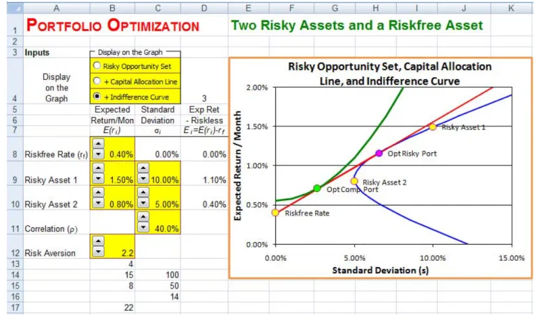
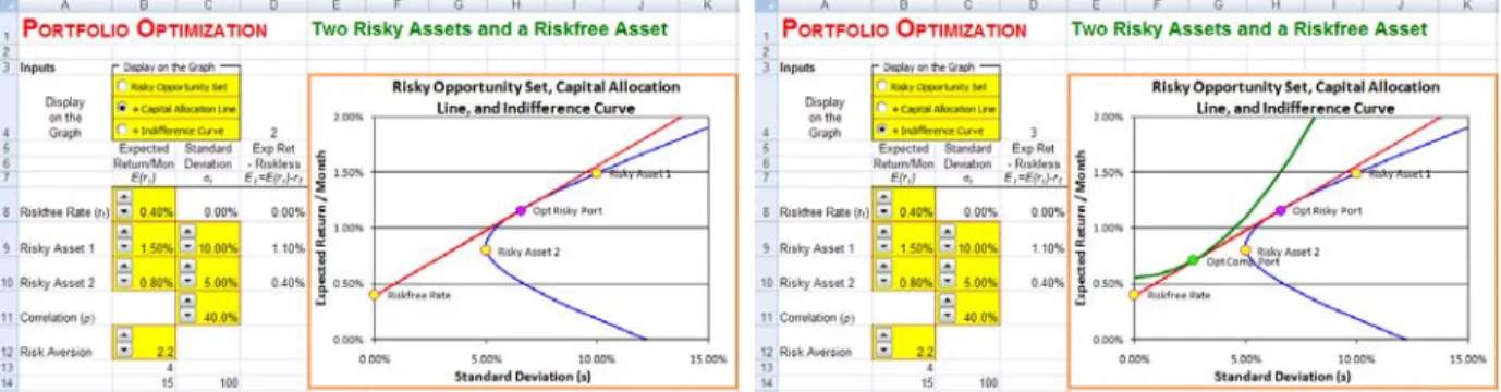
7.1 Two Risky Assets and a Riskfree Asset
Problem. The one-month riskfree rate is 0.40%. Risky Asset 1 has a mean return / month of 1.50% and a standard deviation of 10.00%. Risky Asset 2 has a mean return / month of 0.80% and a standard deviation of 5.0%. The correlation between Risky Asset 1 and 2 is 40.0%. An individual investor with a simple mean and variance utility function has a risk aversion of 2.2. Graph the Risky Opportunity Set, the Optimal Risky Portfolio, the Capital Allocation Line, the investor’s Indifference Curve, and the Optimal Complete Portfolio.
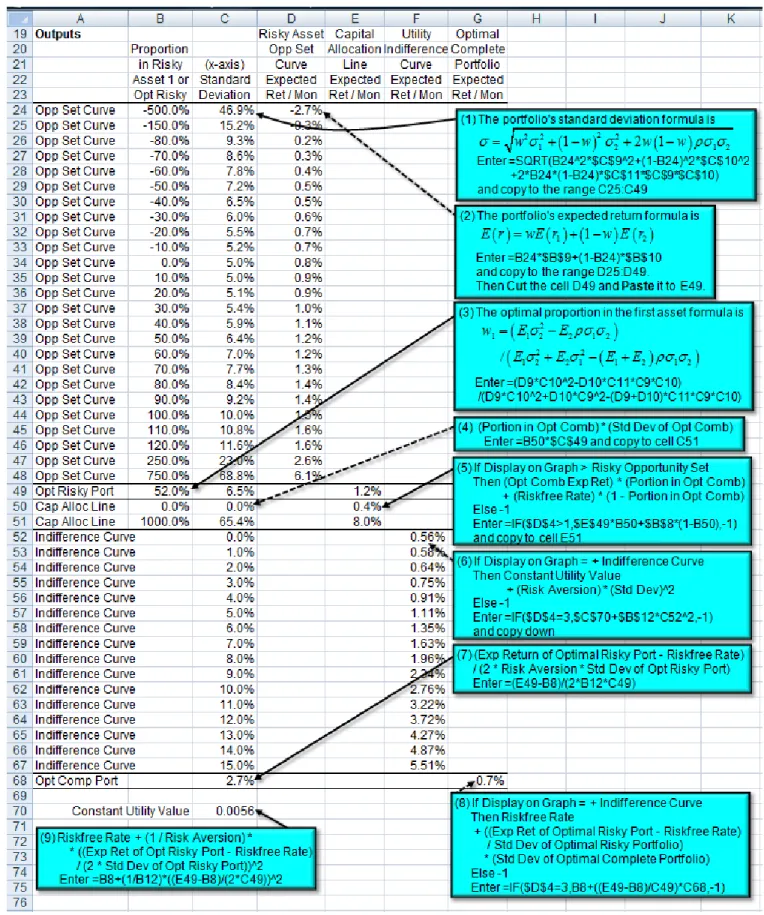
Solution Strategy. The two-asset Risky Opportunity Set involves varying the proportion in the first asset and calculating the portfolio’s standard deviation and expected return. The Optimal Risky Portfolio is computed using a formula for the optimal proportion in the first asset. The Capital Allocation Line comes from any two weights in the Optimal Risky Portfolio. The Optimal Complete Portfolio is computed from a formula for the utility maximizing standard deviation. Then, the Indifference Curve through the Optimal Complete Portfolio is computed.
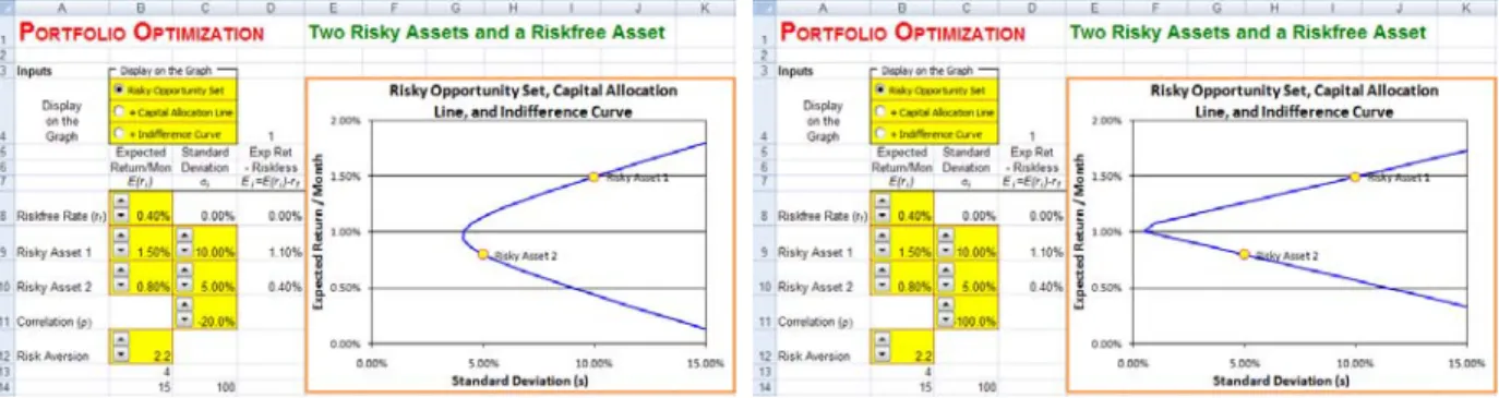
To focus on the two-asset Risky Opportunity Set, click on the Risky Opportunity Set option button. An interesting experiment is to click on the Correlation spin button to raise or lower the correlation.
FIGURE 7.3 Two Assets – Correlation of -20.0% and -100.0%
As the correlation is lowered, the Risky Opportunity Set shifts to the left permitting portfolios with lower standard deviations. At the extreme, a correlation of -100% permits a zero standard devivation (i.e., the Risky Opportunity Set should touch the y-axis). The graph would indeed touch y-axis if additional points in the vicinity were graphed.
FIGURE 7.4 Two Assets – Correlation of +70.0% and +100.0%
As the correlation is raised, the Risky Opportunity Set shifts to the right. At the other extreme, when the correlation is +100%, then the Risky Opportunity Set is a straight line.
Click on the +Capital Allocation Line option button to add the Capital Allocation Line and the Optimal Risky Portfolio. Click on the +Indifference
Curve option button to add the Indifference Curve and the Optimal Complete
FIGURE 7.5 +Capital Allocation Line and +Indifference Curve
An interesting experiment is to click on the Risk Aversion down-arrow spin button to lower the investor’s risk aversion.
FIGURE 7.6 Two Assets – Risk Aversion of 1.0 and 0.5
As risk aversion decreases, the Optimal Complete Portfolio slides up the Capital Allocation Line.
7.2 Descriptive Statistics
Mean-variance optimization is a very useful technique that can be used to find the optimal portfolio investment for any number of risky assets and any type of risky asset: stocks, corporate bonds, international bonds, real estate, commodities, etc. The key inputs required are the means, standard deviations, and correlations of the risky assets and the riskfree rate. Of course,these inputs must be estimated from historical data.
One approach to estimating the inputs is to use descriptive statistics. That is, use the sample means, sample standard deviations, and sample correlations. A serious limitation of this approach is that it assumes that past winners will be future winners and past losers will be future losers. Not surprisingly, the portfolio optimizer concludes that you should heavily buy past winners and heavily short-sell past losers. Given strong evidence that future returns are independent of past returns, then chasing past winners is a fruitless strategy.
A better approach is to estimate an asset pricing model (see the asset pricing chapter), use the estimated model to forecast the future expected return of each asset, and then use these forecasted means in the portfolio optimization. This has the significant advantage of eliminating past idiosyncratic realizations (both positive and negative) from future forecasts. It is especially advantageous to eliminate past idiosyncratic realizations at all three levels: firm-specific, industry/sector-specific, and country-specific. This approach is limited if the asset pricing model has poor forecast power (e.g., the static CAPM). It is desirable to use asset pricing models with higher forecast power (check the R2 of each model in the asset pricing chapter).
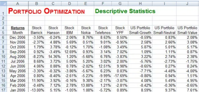
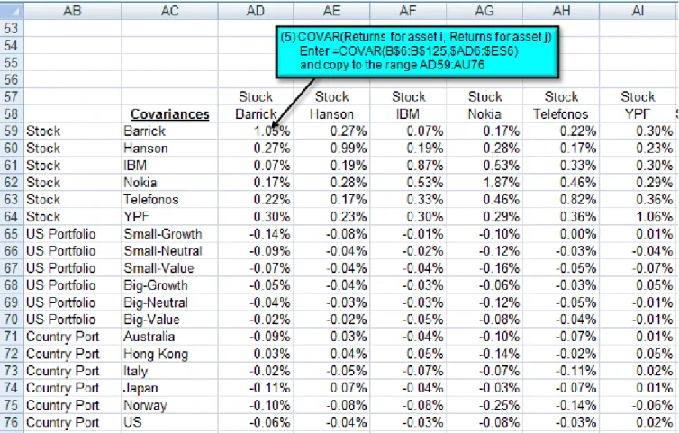
A useful technique for greatly reducing the influence of past idiosyncratic realizations is to analyze portfolios. Therefore, we will use three asset types: individual stocks, broad U.S. portfolios, and country portfolios. The individual stocks include all idiosyncratic realizations. The broad U.S. portfolios have eliminated firm-specific realizations, but still have industry/sector-specific realizations and U.S.-specific realizations. The country portfolios have eliminated firm-specific realizations and mostly eliminated industry/sector-specific realizations, but each country portfolio still has own-country realizations. The individual stocks are Barrick, Hanson, IBM, Nokia, Telephonos, and YPF. They were picked using 1996 (pre-sample) information to avoid selection bias. IBM was the highest volume US stock on the NYSE in 1996. The other five firms were the five highest volume foreign stocks cross-listed on the NYSE in 1996 after disallowing additional firms in the same industry. The US portfolios are six Fama-French portfolios formed by size and by book/market. For example, Small-Growth is an equally-weighted portfolio created from all NYSE/AMEX/NASDAQ firms that have both a small market capitalization and a low book value / market value ratio. Similarly, Big-Value is an equally-weighted portfolio of firms that have both a big market capitalization and a high book value / market value ratio. The country portfolios, created by Fama and French, are broadly-diversified portfolios of firms in each country. The six country portfolios are for Australia, Hong Kong, Italy, Japan, Norway, and the US. The monthly returns for all risky assets are computed from prices in US dollars that are adjusted for stock splits and dividends.
Problem. Given monthly returns for stocks, U.S. portfolios, and country
portfolios, estimate the means, standard deviations, correlations, and variances/covariances among the risky assets. Given the U.S riskfree rate, compute the mean riskfree rate.
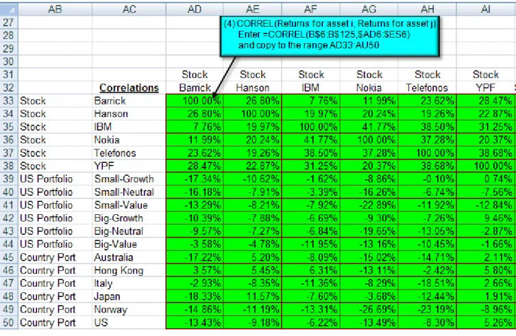
Solution Strategy. Monthly returns for 10 years are provided (see below). Each asset goes down a column. Use TRANSPOSE entered as an Excel matrix to transpose the monthly returns so that each asset goes across a row. This allows convenient computation of the correlation matrix. Specifically, you compute the correlation between one asset going down the column and another asset going across the row. The same approach works for the variance/covariance matrix. Compute the sample descriptive statistics using Excel’s AVERAGE, STDEV, CORREL, and COVAR functions.
The starting point is the monthly returns for each asset.
FIGURE 7.7 Excel Model of Portfolio Optimization – Descriptive Statistics
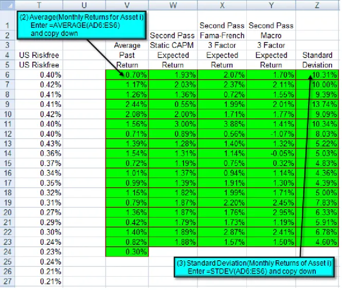
For computational convenience, transpose the monthly returns.
Compute the sample average and sample standard deviation. Columns W to Y contain the forecasted expected return based on various asset pricing models (Static CAPM, Fama-French 3 Factor, and Macro 3 Factor). See the Asset Pricing chapter for details on how these forecasts were made.
FIGURE 7.11 Excel Model of Portfolio Optimization – Descriptive Statistics
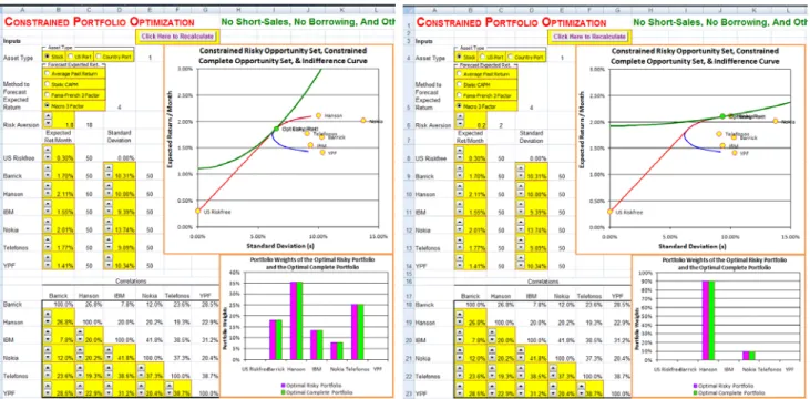
7.3 Many Risky Assets and a Riskfree Asset
Problem. An individual investor with a simple mean and variance utility
function has a risk aversion of 2.8. This investor is considering investing in the given individual stocks, US portfolios, or country portfolios. This investor considers four methods to forecast expected returns: average past return, Static CAPM, Fama-French 3 Factor, or Macro 3 Factor. Determine the Portfolio Weights of the Optimal Risky Portfolio and the Optimal Complete Portfolio. Solution Strategy. To compute the many-asset Risky Opportunity Set, vary the portfolio expected return from 0.00% to 3.00% in increments of 0.10%. Then compute the corresponding portfolio’s standard deviation on the Risky Opportunity Set using the analytic formula. The Optimal Risky Portfolio is computed using a many-asset formula. The Capital Allocation Line comes from any two weights in the Optimal Risky Portfolio. The Optimal Complete Portfolio is computed from a many-asset formula for utility maximization. Then, the Indifference Curve through the Optimal Complete Portfolio is computed.
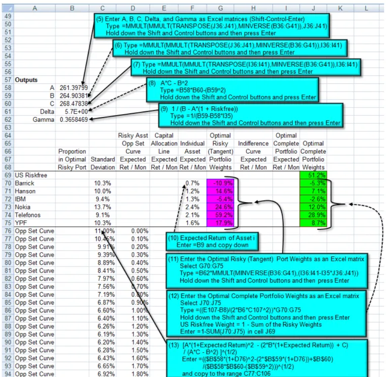
FIGURE 7.14 Excel Model Details of Portfolio Optimization - Many Assets.
Hyperbola Coefficients. In a Mean vs. Standard Deviation graph, the Risky Opportunity Set is a hyperbola. The exact location of the hyperbola is uniquely
determined by three coefficients, usually called A, B, and C. The derivation of the formulas can be found in Merton (1972).4
FIGURE 7.15 Excel Model Details of Portfolio Optimization - Many Assets.
4 See Robert C. Merton, "An Analytic Derivation of the Efficient Portfolio
Frontier," Journal of Financial and Quantitative Analysis, September 1972, pp. 1851-72. His article uses slightly different notation.
The graphs show several interesting things. First, click on Stocks and click on various option buttons for the Method to Forecast Expected Return.
FIGURE 7.16 Average Past Returns and Static CAPM
FIGURE 7.17 Fama-French 3 Factor and Macro 3 Factor
Barrick had a low average return from 1997 – 2006 (0.70%/month), so the Average Past Return method results in a negative portfolio weight on Barrick in the Optimal Risky and Complete Portfolios. However, the three methods based on asset pricing models forecast much higher returns for Barrick ranging from
1.20%/month to 2.07%/month. Hence all three asset pricing based methods result in positive portfolio weights on Barrick in the Optimal Risky and Complete Portfolios. This demonstrates that asset pricing based methods eliminate firm-specific past realizations, which are not generally predictive of future returns. Another point is that the Method to Forecast Expected Return matters a great deal. The four methods produce very different portfolio weights for the Optimal Risky and Complete Portfolios.
An interesting experiment is to click on the Risk Aversion down-arrow spin button to lower the investor’s risk aversion.
FIGURE 7.18 Risk Aversion of 1.9 and 1.3
As risk aversion decreases, the Optimal Complete Portfolio slides up the Capital Allocation Line. When it reaches the Optimal Risky Portfolio, then the Optimal Complete Portfolio involves putting 0% in the riskfree asset and 100% in the Optimal Risky Portfolio. As risk aversion decreases further, it slides above the Optimal Risky Portfolio, then the Optimal Complete Portfolio involves a negative weigh in the riskfree asset (e.g., borrowing) and “more than 100%” in the Optimal Risky Portfolio.
Return risk aversion to 2.8 and imagine that you did security analysis on Barrick. Click on the Barrick Expected Return/Month up-arrow spin button to raise expected return/month to 2.30% (e.g., Barrick is underpriced). Then try the opposite experiment by clicking on the Barrick Expected Return/Month down-arrow spin button to lower expected return/month to 2.30% (e.g., Barrick is overpriced).
FIGURE 7.19 Barrick Expected Return/Month of 2.60% and 0.90%
When Barrick’s Expected Return/Month increases to 2.60%, the Optimal Risky Portfolio weight in Barrick rises dramatically (to 33.4%) to exploit this higher return. But also notice that the Optimal Risky Portfolio does NOT put 100% in Barrick even though it has the highest expected return of all assets considered. The Optimal Risky Portfolio maintains an investment in all five risk assets in order lower the portfolio standard deviation by diversification. Thus, the Optimal Risky Portfolio is always a trade-off between putting a higher weight in assets with higher returns vs. spreading out the investment to lower portfolio risk. When Barrick’s Expected Return/Month decreases to 0.90%, the Optimal Risky Portfolio weight in Barrick declines so far that it even goes negative (to -5.0%) to exploit this low return. A negative portfolio weight means short-selling. Putting a -5.0% in low return asset raises the overall portfolio return by allowing 105% to be invested in high return assets.
Return Barrick’s Expected Return/Month to 1.70% and consider changes in Standard Deviation. Click on the IBM Standard Deviation down-arrow spin button to lower the standard deviation to 5.39%. Then try the opposite experiment by clicking on the IBM Standard Deviation up-arrow spin button to raise the standard deviation to 12.39%.
FIGURE 7.20 IBM Standard Deviation of 5.39% and 12.39%
When IBM’s Standard Deviation falls to 5.39%, the Optimal Risky Portfolio weight in IBM rises dramatically (to 59.9%) to exploit this low risk. But also notice that the Optimal Risky Portfolio does NOT put 100% in IBM even though it has the lowest standard deviation. It still pays to maintain some investment in all five risk assets in order lower the portfolio standard deviation by diversification. When IBM’s Standard Deviation rises to 12.39%, the Optimal Risky Portfolio weight in IBM falls dramatically (to 2.2%) to avoid this high risk.
Return IBM’s Standard Deviation to 9.39% and consider changes in Correlation. Click on the Barrick/Telefonos Correlation down-arrow spin button (in cell B22) to lower the correlation to -36.4%. Then try the opposite experiment by clicking on the Barrick/Telefonos Correlation up-arrow spin button to raise the correlation to 63.6%.
FIGURE 7.21 Barrick/Telefonos Correlation of -36.4% and 63.6%
When Barrick/Telefonos’ Correlation falls to -36.4%, the Optimal Risky Portfolio weight in both Barrick and Telefonos rises dramatically (Barrick to 41.4% and Telefonos to 52.1) to exploit this low correlation. When Barrick/Telefonos’ Correlation rises to -63.6%, the Optimal Risky Portfolio weight in both Barrick and Telefonos falls dramatically (Barrick to 12.7% and Telefonos to 20.1) to avoid this high correlation.
Return Barrick/Telefonos’ Correlation to 23.6% and consider changes in the Riskfree Rate. Click on the US Riskfree Expected Return/Month up-arrow spin button to raise the Riskfree Rate to 1.10%. Then try the opposite experiment by clicking on the US Riskfree Expected Return/Month down-arrow spin button to lower the Riskfree Rate to 0.02%.
FIGURE 7.22 US Riskfree Rate of 1.10% and 0.02%
When the US Riskfree Rate increases to 1.10%, the Risky Opportunity Set (the blue curve) stays the same and Capital Allocation Line (the red line) slides up it, such that the Optimal Risky Portfolio (the purple dot) slides up the Risky Opportunity Set. This higher position means that Optimal Risky Portfolio increases the weights on high expected return assets like Hanson. When the US Riskfree Rate decreases to 0.02%, Capital Allocation Line slides down the Risky Opportunity Set, such that the Optimal Risky Portfolio slides down the Risky Opportunity Set. This lower position means that Optimal Risky Portfolio spreads its weights more evenly across all five assets.
Return the US Riskfree Rate to 0.30% and consider portfolios. Click on Fama-French 3 Factor and click on US Port. Next, click on Country Port.
FIGURE 7.23 US Portfolios and Country Portfolios
Notice that the Risky Opportunity Set shifts far to the left. This is because the standard deviations for US Portfolios and County Portfolios are much smaller than Individual Stocks. Roughly, the portfolio standard deviations are half as big as the individual stock standard deviations. This demonstrates the impact of portfolio diversification in eliminating firm-specific risk.
Again, using portfolios matters a great deal. The US Portfolios and County Portfolios produce very different portfolio weights for the Optimal Risky and Complete Portfolios than the Individual Stocks.
Problems
1. The one-month riskfree rate is 0.23%. Risky Asset 1 has a mean return / month of 2.10% and a standard deviation of 13.00%. Risky Asset 2 has a mean return / month of 1.30% and a standard deviation of 8.0%. The correlation between Risky Asset 1 and 2 is 20.0%. An individual investor with a simple mean and variance utility function has a risk aversion of 2.0. Graph the Risky Opportunity Set, the Optimal Risky Portfolio, the Capital Allocation Line, the investor’s Indifference Curve, and the Optimal Complete Portfolio.
2. Download 10 years of monthly returns for stocks, U.S. portfolios, or country portfolios of your choice and estimate the means, standard deviations, correlations, and variances/covariances among the risky assets. Download 10 years of the U.S riskfree rate, compute the mean riskfree rate.
3. An individual investor with a simple mean and variance utility function has a risk aversion of 1.5. This investor is considering investing in the assets you
downloaded for problem 2. This investor considers four methods to forecast expected returns: average past return, Static CAPM, Fama-French 3 Factor, or Macro 3 Factor. Determine the Portfolio Weights of the Optimal Risky Portfolio and the Optimal Complete Portfolio.