Fuzzy clustering with Minkowski distance
functions
Patrick J.F. Groenen
∗Uzay Kaymak
†Joost van Rosmalen
‡July 6, 2006
Econometric Institute Report EI 2006-24
Abstract
Distances in the well known fuzzy c-means algorithm of Bezdek (1973) are measured by the squared Euclidean distance. Other dis-tances have been used as well in fuzzy clustering. For example, Jajuga (1991) proposed to use the L1-distance and Bobrowski and Bezdek (1991) also used the L∞-distance. For the more general case
of Minkowski distance and the case of using a root of the squared Minkowski distance, Groenen and Jajuga (2001) introduced a ma-jorization algorithm to minimize the error. One of the advantages of iterative majorization is that it is a guaranteed descent algorithm, so that every iteration reduces the error until convergence is reached. However, their algorithm was limited to the case of Minkowski pa-rameter between 1 and 2, that is, between the L1-distance and the Euclidean distance. Here, we extend their majorization algorithm to any Minkowski distance with Minkowski parameter greater than (or equal to) 1. This extension also includes the case of theL∞-distance.
We also investigate how well this algorithm performs and present an empirical application.
∗Econometric Institute, Erasmus University Rotterdam, P.O. Box 1738, 3000 DR
Rot-terdam, The Netherlands, groenen@few.eur.nl).
†kaymak@few.eur.nl
1
Introduction
Since Ruspini (1969) first proposed the idea of fuzzy partitions, fuzzy clus-tering has grown to be an important tool for data analysis and modelling. Especially after the introduction of the fuzzyc-means algorithm (Dunn, 1973; Bezdek, 1973), objective function-based fuzzy clustering has received much attention from the scientific community as well as the practitioners of fuzzy set theory (Bezdek & Pal, 1992; Yang, 1993; Baraldi & Blonda, 1999a, 1999b; H¨oppner, Klawonn, Kruse, & Runkler, 1999). Consequently, fuzzy clustering has been applied extensively for diverse tasks such as pattern recognition, data analysis, data mining, image processing, and engineering systems de-sign. Objective function-based fuzzy clustering has also become one of the key techniques in fuzzy modelling, where they are used for partitioning the feature space from which the rules of a fuzzy system can be derived (Babuˇska, 1998).
In general, objective function-based fuzzy clustering algorithms partition a data set into overlapping groups by minimizing an objective function de-rived from the distance between the cluster prototypes and the data points (or objects). The clustering results are largely influenced by how this distance is computed, since it determines the shape of the clusters. The success of fuzzy clustering in various applications may depend very much on the shape of the clusters. As a result, there is a significant amount of literature on fuzzy clustering, which is aimed at investigating the use of different distance functions in fuzzy clustering, leading to different cluster shapes.
One way of influencing the shape of the clusters is to consider prototypes with a geometric structure. The fuzzyc-varieties (FCV) algorithm uses linear subspaces of the clustering space as prototypes (Bezdek, Coray, Gunderson, & Watson, 1981b), which is useful for detecting lines and other linear struc-tures in the data. The fuzzy c-elliptotypes (FCE) algorithm takes convex combinations of fuzzy c-varieties prototypes with fuzzy c-means prototypes to obtain localized clusters (Bezdek, Coray, Gunderson, & Watson, 1981a). Kaymak and Setnes (2002) proposed using volumes in the clustering space as the cluster prototypes.
Another way for influencing the shape of the clusters is modifying the distance measure that is used in the objective function. Distances in the well known fuzzy c-means algorithm of Bezdek (1973) are measured by the squared Euclidean distance. Gustafson and Kessel (1979) use the quadratic Mahanalobis norm to measure the distance. Jajuga (1991) proposed to use theL1-distance and Bobrowski and Bezdek (1991) also used theL∞-distance.
Further, Hathaway, Bezdek, and Hu (2000) studied the Minkowski semi-norm as the dissimilarity function.
In this paper, we consider fuzzy clustering with the more general case of the Minkowski distance and the case of using a root of the squared Minkowski distance. The Minkowski norm provides a concise, parametric distance func-tion that generalizes many of the distance funcfunc-tions used in the literature. The advantage is that mathematical results can be shown for a whole class of distance functions, and the user can adapt the distance function to suit the needs of the application by modifying the Minkowski parameter. By con-sidering the additional case of the roots of the squared Minkowski distance, we introduce an extra parameter that can be used to control the behaviour of the clustering algorithm with respect to outliers. This provides an addi-tional way of dealing with outliers, which is different than the “noise cluster” approach proposed in Dave (1991).
Our analysis follows the approach that Groenen and Jajuga (2001) in-troduced previously. Minimization of the objective function is partly done by iterative majorization. One of the advantages of iterative majorization is that it is a guaranteed descent algorithm, so that every iteration reduces the objective function until convergence is reached. The algorithm in Groenen and Jajuga (2001) was limited to the case of a Minkowski parameter be-tween 1 and 2, that is, bebe-tween the L1-distance and the Euclidean distance.
Here, we extend their majorization algorithm to any Minkowski distance with Minkowski parameter greater than (or equal to) 1. This extension also includes the case of the L∞-distance. We also explore the behaviour of our algorithm with an illustrative example using real-world data.
The outline of the paper is as follows. We expose the formalization of the clustering problem in Section 2. The majorizing algorithm for fuzzy c-means with Minkowski distances is given in Section 3. We discuss in Section 4 the behaviour of our algorithm by using an illustrative example based on empirical data concerning attitudes about the Internet. Finally, conclusions are given in Section 5.
2
Formalization
In this paper, we focus on the fuzzy clustering problem that uses a root of the squared Minkowski distance. This problem can be formalized by minimizing the objective (or loss) function
L(F,V) = n X i=1 K X k=1 fiksd2ikλ(V) (1)
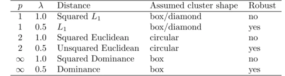
Table 1: Special distances obtained by specific choice of λ and p and some of their properties.
p λ Distance Assumed cluster shape Robust
1 1.0 SquaredL1 box/diamond no
1 0.5 L1 box/diamond yes
2 1.0 Squared Euclidean circular no
2 0.5 Unsquared Euclidean circular yes
∞ 1.0 Squared Dominance box no
∞ 0.5 Dominance box yes
under the constraints
0≤fik ≤1, i= 1, ..., n k = 1, ..., K
PK
k=1fik = 1, i= 1, ..., n (2)
wherenis the number of objects,K is the number of fuzzy clusters,fikis the membership grade of object i in fuzzy clusterk,s is the weighting exponent larger than 1. The distance between object i given by the i-th row of the
n×m data matrix X and fuzzy cluster k of the K ×m cluster coordinate matrix V is given by d2λ ik(V) = Ã m P j=1|xij −vkj| p !2λ/p , 1≤p≤ ∞, 0≤λ≤1 (3)
where λ is the power of the squared Minkowski distance d2λ
ik(V) with 1 ≤
p≤ ∞.
The introduction of the powerλallows to control the loss function against outliers. For large λ, e.g., λ = 1, outliers may dominate the loss function, whereas the loss function will be more robust if λ is small.
The use of Minkowski distances allows to vary the assumptions of the shape of the clusters by varying p. The most often used value is p= 2 that assumes a circular cluster shape. Usingp= 1 assumes that the clusters are in the shape of a (rotated) square in two dimensions or a diamond like shape in three or more dimensions. For p=∞, the clusters are assumed to be in the form of a box with sides parallel to the axes. Both p= 1 and p=∞ can be used in cases where the data structures have “boxy” shapes, i.e., shapes with sharp “edges” (Bobrowski & Bezdek, 1991). A summary of combinations of
λ andpand some properties of the distances are presented in Table 1 (taken from Groenen and Jajuga 2001).
Groenen and Jajuga (2001) note that (1) has several known fuzzy clus-tering models as a special case. For example, for p = 2 and λ = 1, the
important member of fuzzy isodata family is obtained that corresponds to squared Euclidean distances (while assuming the identity metric). A fuzzy clustering objective function that is robust against outliers can be obtained by choosing λ= 1/2 and p= 1 so that the L1-norm is used. Note that this
choice implicitly assumes a “boxy” shape of the clusters. A robust version of fuzzy clustering with a circular shape can be specified by λ = 1/2 and
p = 2 that implies the unsquared Euclidean distance. Thus, λ takes care of robustness issues and p of the shape of the clusters. Dodge and Rousson (1998) named the cluster centroids for λ = 1/2 and p= 1 ‘L1-medians’, for
λ = 1 and p = 1 ‘L1-means’, for λ = 1/2 and p = 2 ‘L2-medians’, and for
λ = 1 andp= 2 the well known ‘L2-means’.
3
The Majorizing Algorithm for Fuzzy
c
-means with Minkowski Distances
Depending on the particular function, the minimization method of itera-tive majorization has some nice properties. The most important one is that in each iteration of the iterative majorization the loss function is decreased until this value converges. Such guaranteed descent methods are useful because no step in the wrong direction can be taken. Note that this property does not imply that a global minimum is found unless the function exhibits a special property such as convexity. Some general papers on iterative majorization are De Leeuw (1994), Heiser (1995), Lange, Hunter, and Yang (2000), Kiers (2002), and Hunter and Lange (2004); an introduction can be found in Borg and Groenen (2005).
The majorization algorithm of Groenen and Jajuga (2001) worked for all 1 ≤ p ≤ 2. Below we expand their majorization algorithm to the situation of all p > 1. Each iteration of their algorithm consists of two steps: (1) update the cluster memberships Ffor fixed centers V and (2) updateV for fixed F. For Step (2) we use majorization. Below, we start by explaining some basic ideas of iterative majorization. Then, the update of the cluster memberships is given. This is followed by some derivations for the update of the cluster centers V in the case of 1≤ p≤ 2. Then, the update is derived for 2< p <∞ and a special update for the case of p=∞.
3.1
Iterative Majorization
Iterative majorization can be seen as a gradient method with a fixed step size. However, iterative majorization can also be applied to functions that
are at some points nondifferentiable. Central to iterative majorization is the use of an auxiliary function similar to the first order Taylor expansion used as an auxiliary function in a gradient method and second order expansion for Newton’s method. The unique feature of the auxiliary function in itera-tive majorization—the so-called majorizing function— is that it touches the original function or is located above it. In contrast, the auxiliary functions of the gradient method or Newton’s method can be partially below and above the original function.
Let the original function be presented by ϕ(X), the majorizing function by ˆϕ(X,Y), where Y is the current known estimate. Then, a majorizing function has to fulfil the following three requirements: (1) ˆϕ(X,Y) is a more simple function inXthanϕ(X), (2) it touchesϕ(X) at the known supporting point Y so that ϕ(Y) = ˆϕ(Y,Y), and (3) ˆϕ(X,Y) is never smaller than
ϕ(X), that is, ϕ(X)≤ ϕˆ(X,Y) for all X. Often, the majorizing function is either linear or quadratic.
To see how a single iteration reduces ϕ(X), consider the following. Let
Y be some known point and let the minimum of the majorizing function ˆ
ϕ(X,Y) be given by X+. Note that for a majorizing algorithm to be suffi-ciently fast, it should be easy to computeX+. Because the ˆϕ(X,Y) is always
larger than or equal to the ϕ(X), we must have ϕ(X+) ≤ ϕˆ(X+,Y). This property is essential for the so-called sandwich inequality, that is, the chain
ϕ(X+)≤ϕˆ(X+,Y)≤ϕˆ(Y,Y) = ϕ(Y) (4)
that proves that the update X+ never increase the original function. For the next iteration, we simply set Y equal to X+ and compute a new majorizing
function. For functions that are bounded from below or are sufficiently con-strained, the majorization algorithm always gives a convergent sequence of nonincreasing function values, see, for example, Borg and Groenen (2005).
One property that we use here is that if a function consists of a sum of functions and that each of these functions can be majorized, then the sum of the majorizing functions also majorizes the original functions. For example, suppose thatϕ(X) =Piϕi(X) andϕi(X)≤ϕˆi(X,Y) thenϕ(X)≤ P
iϕˆi(X,Y).
3.2
Updating the Cluster Membership
For fixed cluster centersV, Groenen and Jajuga (2001) derive the update of the cluster memberships Fas
fik = ³ d2λ ik(V) ´−1/(s−1) PK l=1 ³ d2λ il (V) ´−1/(s−1) (5)
for fixed V and s > 1, see also Bezdek (1973). These memberships are derived by taking the Lagrangian function, setting the derivatives equal to zero, and solving the equations.
There are two special cases. The first one occurs ifsis large. The largers, the closer−1/(s−1) approaches zero. As a consequence³d2λ
ik(V)
´−1/(s−1)
≈1 for all ik so that update (5) will yield fik ≈ 1/K. Numerical accuracy can
produce equal cluster memberships, even for not too large s, such as,s= 10. If this happens for all fik, then all cluster centers collapse into the same point and the algorithm gets stuck. Therefore, in practical applications s
should be chosen quite small, say, s ≤ 2. The second special case occurs if
s approaches 1 from above. In that case, update (5) approaches the update for hard clustering, that is, setting
fik =
(
1 if dik = minldil
0 if dik 6= minldil, (6)
where it is assumed that minldil is unique.
3.3
Updating the Cluster Coordinates
We follow the majorization approach of Groenen and Jajuga (2001) for find-ing an update of the cluster coordinates V for fixed F. Our loss function
L(F,V) may be seen as a weighted sum of theλth root of squared Minkowski distances. Because the weightsfs
ikare nonnegative, it suffices for now to
con-sider d2λ
ik(V), the root of squared Minkowski distances. Let us focus on the
root for a moment. Groenen and Heiser (1996) proved that for root λ of a, with 0≤λ≤1,a≥0 andb >0, the following majorization inequality holds:
aλ ≤(1−λ)bλ +λbλ−1a, (7)
with equality if a=b. Using (7), we can obtain the majorizing inequality
d2λ
ik(V) ≤ (1−λ)d2ikλ(W) +λd
2(λ−1)
ik (W)d2ik(V), (8)
with W is the estimate of V from the previous iteration and we assume for the moment that dik(W) > 0. Thus, the root λ of a squared Minkowski distance can be majorized by a constant plus a positive weight times the squared Minkowski distance.
The next step is to majorize the squared Minkowski distance. To do so, we distinguish three cases: (a) 1≤p≤2, (b) 2< p <∞, and (c) p=∞.
For the case of 1 ≤ p ≤ 2, Groenen and Jajuga (2001) use H¨older’s inequality to prove that
d2 ik(V) ≤ Pm j=1(xij −vkj)2|xij −wkj|p−2 dpik−2(V) = m X j=1 a(1ijk≤p≤2)(xij −vkj)2, = m X j=1 a(1ijk≤p≤2)v2 kj−2 m X j=1 b(1ijk≤p≤2)vkj+c(1ik≤p≤2) (9) where a(1ijk≤p≤2) = |xij −wkj|p−2 dpik−2(V) ,
b(1ijk≤p≤2) = a(1ijk≤p≤2)xij,
c(1ik≤p≤2) =
m X
j=1
a(1ijk≤p≤2)x2ij.
For p ≥ 2, (9) is reversed, so that it cannot be used for majorization. However, Groenen, Heiser, and Meulman (1999) have developed majorizing inequalities for squared Minkowski distances with 2 < p < ∞ and p =
∞. We first look at 2 < p < ∞. They proved that the Hessian of the squared Minkowski distance always has the largest eigenvalue smaller than 2(p−1). By numerical experimentation they even found a smaller maximum eigenvalue of (p−1)21/p but they were unable to prove this. Knowing an
upper bound of the largest eigenvalue of the Hessian is enough to derive a majorizing inequality if it is combined with the requirement of touching at the supporting point (that is, at this point the gradients of the squared Minkowski distance and the majorizing function must be equal and the same must hold for their function values).
This majorizing inequality can be derived as follows. For notational sim-plicity, we express the squared Minkowski distance as d2(t) = (P
j|tj|p)2/p.
The first derivative∂d2(t)/∂t
j can be expressed as 2tj|tj|p−2/dp−2(t).
Know-ing that the largest eigenvalue of the Hessian of d2(t) is bounded by 2(p−1),
a quadratic majorizing can be found (Groenen et al., 1999) of the form
d2(t) ≤ 4(p−1)Xm j=1 t2 j −2 m X j=1 tjbj+c with bj = 4(p−1)uj − 1 2 ∂d2(u) ∂uj =uj " 4(p−1)− |uj| p−2 dp−2(u) # ,
c = d2(u) + 4(p−1) m X j=1 u2j − m X j=1 uj∂d 2(u) ∂uj = 4(p−1) m X j=1 u2j −d2(u),
and u the known current estimate of t. Substituting tj = xij − vkj and uj =xij −wkj gives the majorizing inequality
d2 ik(V) ≤ 4(p−1) m X j=1 (xij −vkj)2 −2 m X j=1 (xij −vkj)(xij−wkj)[4(p−1)− |xij −wkj|p−2/dpik−2(W)] +4(p−1) m X j=1 (xij −wkj)2−dik(W).
Some rewriting yields
d2 ik(V)≤a(2<p<∞) m X j=1 v2 kj −2 m X j=1 b(2ijk<p<∞)vkj + m X j=1 c(2ijk<p<∞), (10) where a(2<p<∞) = 4(p−1) b(2ijk<p<∞) = a(2<p<∞)w kj−(xij −wkj)|xij −wkj|p−2/dpik−2(W) c(2ik<p<∞) = a(2<p<∞)Xm j=1 w2 kj−d2ik(W) + 2 m X j=1 xij(xij −wkj)|xij −wkj|p−2/dpik−2(W).
Ifpgets larger, a(2<p<∞) also becomes larger, thereby making the majorizing
function steeper. As a result, the steps taken per iteration will be smaller. For the special case of p=∞, Groenen et al. (1999) also provided a majorizing inequality. This one can be (much) faster than using (10) with a large p. It depends on the difference between the two largest values of |xij −wkj| over
the different j.
Let us for the moment focus on d2(t) again. And letϕj be an index that
orders the values |tj| decreasingly, so that |tϕ1| ≤ |tϕ2| ≤ . . . ≤ |tϕm|. The
majorizing function for p=∞becomes
d2(t) ≤ a m X j=1 t2j −2 m X j=1 tjbj+c with a = |uϕ1| |uϕ1| − |uϕ2| if |uϕ1| − |uϕ2|> ε ²+|uϕ1| ε if |uϕ1| − |uϕ2| ≤ε
bj = a|uϕ2|uj |uj| if j =ϕ1 auj if j 6=ϕ1 c = d2(u) + 2X j ujbj −a X j u2 j.
Note that the definition ofafor|uϕ1|−|uϕ2| ≤εtakes care of ill conditioning,
that is, values of a getting too large. Strictly speaking, majorization is not valid anymore, but for small enough² the monotone convergence is retained. Backsubstitution oftj =xij−vkj anduj =xij−wkj gives the majorizing
inequality d2 ik(V) ≤ a(ikp=∞) X j (xij−vkj)2−2 X j (xij −vkj)bijk(p=∞)+c(ikp=∞) = a(ikp=∞)X j vkj2 −2X j vkjb(ijkp=∞)+c(ikp=∞) (11) where a(ikp=∞) = |xiϕ1 −wkϕ1| |xiϕ1 −wkϕ1| − |xiϕ2 −wkϕ2| if |xiϕ1 −wkϕ1| − |xiϕ2 −wkϕ2|> ε, ε+|xiϕ1 −wkϕ1| ε if |xiϕ1 −wkϕ1| − |xiϕ2 −wkϕ2| ≤ε, b(ijkp=∞) = a(ikp=∞) · xij − |xiϕ2 −|xwkϕ2|(xiϕ1 −wkϕ1) iϕ1 −wkϕ1| ¸ if j =ϕ1, a(ikp=∞)wkj if j 6=ϕ1, c(ikp=∞) = d2ik(W)−2X j b(ijkp=∞)(xij −wkj)− X j a(ikp=∞)wkj2 + 2X j a(ikp=∞)x2ij.
Recapitulating, the loss function is a weighted sum of the root of the squared Minkowski distance. The root can be majorized by (8) that yields a function of squared Minkowski distances. For the case 1 ≤ p ≤ 2, (9) shows how the squared Minkowski distance can be majorized by a quadratic function in V (see, Figure 1), (10) how this can be done for 2 < p < ∞, and (11) for p =∞. These results can be combined to obtain the following majorizing function for L(F,V), that is,
L(F,V) ≤ λ m X j=1 K X k=1 v2 kj n X i=1 aijk−2λ m X j=1 K X k=1 vkj n X i=1 bijk+c+ n X i=1 K X k=1 cik(12), where aijk = fs ikd2(ikλ−1)(W)aijk(1≤p≤2) if 1≤p≤2 fs ikd2(ikλ−1)(W)a(2<p<∞) if 2< p <∞ fs ikd 2(λ−1) ik (W)a (p=∞) ik if p=∞
bijk = fs ikd 2(λ−1) ik (W)b (1≤p≤2) ijk if 1≤p≤2 fs ikd 2(λ−1) ik (W)b (2<p<∞) ijk if 2< p <∞ fs ikd 2(λ−1) ik (W)b (p=∞) ijk if p=∞ cik = fs ikd 2(λ−1) ik (W)c (1≤p≤2) ik if 1≤p≤2 fs ikd2(ikλ−1)(W)c(2ik<p<∞) if 2< p < ∞ fs ikd 2(λ−1) ik (W)c (p=∞) ik if p=∞ c = n X i=1 K X k=1 fs ik(1−λ)d2ikλ(W).
It is easily recognized that (12) is a quadratic function in the cluster coordinate matrix V that reaches its minimum for
v+ kj = Pn i=1bijk Pn i=1aijk . (13)
3.4
The Majorization Algorithm
The majorization algorithm can be summarized as follows.
1. Given a data set X. Set 0 ≤λ≤ 1, 1≤ p≤ ∞, and s ≥1. Choose ε, a small positive constant.
2. Set the membership gradesF=F0 with 0≤ f0
ik ≤1 and
PK
k=1fik0 = 1
and the cluster coordinate matrix V=V0. ComputeLprev =L(F,V).
3. Update Fby (5) if s >1 or by (6) if s= 1. 4. SetW=V. Update V by (13).
5. Stop if (Lprev−L(F,V))/L(F,V))< ε.
6. SetLprev =L(F,V) and go to Step 3.
4
Internet Attitudes
To show how fuzzy clustering can be used in practice, we apply it to an empirical data set. Our data set is based on a questionnaire on attitudes towards the Internet. It consists of evaluations of 22 statements about the Internet by 194 students gathered around 2002 before the wide availability
a.
b.
c.
Figure 1: The original function d2(t) and the majorizing functions forp= 1,
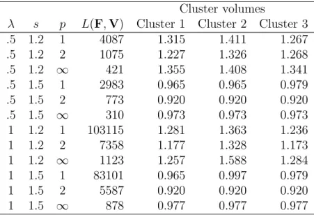
Table 2: Results of fuzzy clustering for internet data set using K = 3. Cluster volumes
λ s p L(F,V) Cluster 1 Cluster 2 Cluster 3
.5 1.2 1 4087 1.315 1.411 1.267 .5 1.2 2 1075 1.227 1.326 1.268 .5 1.2 ∞ 421 1.355 1.408 1.341 .5 1.5 1 2983 0.965 0.965 0.979 .5 1.5 2 773 0.920 0.920 0.920 .5 1.5 ∞ 310 0.973 0.973 0.973 1 1.2 1 103115 1.281 1.363 1.236 1 1.2 2 7358 1.177 1.328 1.173 1 1.2 ∞ 1123 1.257 1.588 1.284 1 1.5 1 83101 0.965 0.997 0.979 1 1.5 2 5587 0.920 0.920 0.920 1 1.5 ∞ 878 0.977 0.977 0.977
of broadband Internet access. The statements were evaluated using a seven-point Likert scale, ranging from 1 (completely disagree) to 7 (completely agree).1
The respondents are clustered using the fuzzy clustering algorithm to study their attitudes towards the Internet. We use K = 3. The convergence criterion ε of the majorization algorithm was set to 10−8. The monotone
convergence of the majorization algorithm generally leads to a local mini-mum. However, depending on the data and the different settings ofp,s, and
λ several local minima may exist. Therefore, in every analysis, we applied 10 random starts and report the best one. We tried three different values of
p (1,2,∞) to examine the cluster shape, two values of s (1.2, 1.5) to study the sensitivity for the fuzziness parameters, and two values forλ(.5, 1.0) to check the sensitivity for outliers.
Table 2 shows some results for this data set using different values forλ, s, and p. The final value of the loss function and the volumes of the three clus-ters are calculated in every instance. As there is no natural standardization for L(F,V), the values can only be used to check for local minima within a particular choice of λ, s, and p.
The labelling problem of clusters refers to possible permutations of the clusters among different runs. To avoid this problem, we took theVobtained
byλ = 1, p= 1, ands= 1.2 as a target solutionV∗ and tried all permutation matrices P of the rows of V (with V(Perm) = PV) for other combinations of λ, p, and s and choose the one that minimizes the sum of the squared residuals X k X j (v∗kj−v(Perm)kj )2 =kV∗−PVk2. (14) The permutation Pthat minimizes (14) is also applied to the cluster mem-berships, so that F(Perm) =FP0. By using this strategy, we assume that the clusters are the same among the different analyses.
To measure the size of a cluster, we consider its volume by computing the cluster covariance matrix with elements
Gk= Pn i=1fiks(xi−vk)0(xi−vk) Pn i=1fiks ,
where xi is the 1×j row vector of row i of X and vk row i of V. Then, as a measure of the volume of cluster k one can use det(Gk). However,
we take det(Gk)1/m, which can be interpreted as the geometric mean of the
eigenvalues of Gk and has the advantage that it is not sensitive to m. Table 2 shows that for s = 1.5 the cluster volumes are all the same with a slight difference among the clusters of p = 1. For s = 1.5, Cluster 2 is generally the largest and the other two have about the same size. The more robust setting of λ=.5, generally shows slightly larger clusters, but the effect does not seem large. Therefore, outliers do not seem to be a problem of this data set.
To interpret the clusters, we have to look at V. As it is impossible to show the clusters in a 22-dimensional space, they are represented by parallel coordinates (Inselberg, 1981, 1997). Every clusterkdefines a line through the cluster centersvkj, see Figure 2 fors= 1.2 andλ= 1. Note that the order of
the variables is unimportant. This figure can be interpreted by considering the variables that have different scores for the clusters. The patterns for
p= 1,2, and ∞ are similar and p= 1 shows them the clearest.
For p = 1 and λ = 1, each cluster center is a (weighted) median of a cluster. Because all elements of the internet data set are integers, the cluster centers necessarily have integer values. The left most panel in Figure 2 shows the parallel coordinates for p= 1. The solid line represents Cluster 1 and is characterized by respondents saying that the Internet is easy, safe, addictive, and who seem to form an active user community (positive answers to variables 16 to 22). However, the strongest difference of Cluster 1 to the others is given by their total rejection of regulation of content on the Internet. We call this
Disagree strongly Neutral Agree strongly Disagree strongly Neutral Agree strongly Disagree strongly Neutral Agree strongly
1. Paying using Internet is safe 2. Surfing the Internet is easy 3. Internet is unreliable 4. Internet is slow 5. Internet is user-friendly
6. Internet is the future’s means of communication 7. Internet is addictive
8. Internet is fast
9. Sending personal data using the Internet is unsafe 10. The prices of Internet subscriptions are high 11. Internet offers many possibilities for abuse 12. The costs of surfing are high
13. Internet offers unbounded opportunities 14. Internet phone costs are high
15. The content of web sites should be regulated 16. Internet is easy to use
17. I like surfing
18. I often speak with friends about the Internet 19. I like to be informed of important new things 20. I always attempt new things on the Internet first 21. I regularly visit websites recommended by others 22. I know much about the Internet
p = 1 p = 2 p = ∞
Figure 2: Parallel coordinates representation of clusters with λ = 1, p = 1, and s= 1.2. The lines correspond to clusters 1 (solid line), 2 (dashed line), and 3 (dotted line).
cluster the experts. Cluster 2 (the dashed line) refers to respondents that are not active users (negative answers to variables 18 to 22), find the Internet not user friendly, unsafe to pay, not addictive, and they are neutral on the issue of regulation of the content of websites. This cluster is called the novices. Cluster 3 looks in some respects like Cluster 1 (surfing is easy, paying is not so safe) but those respondents do not find the Internet addictive, are neutral on the issue of the speed of the Internet connection, and seem to be not such active users as those of Cluster 1. They are mostly characterized by finding the costs of Internet high and allowing for some content regulation. This cluster represents the cost-aware Internet user.
As we are dealing with three clusters and the cluster memberships sum to one, they can be plotted in a triangular 2D scatterplot—called a triplot—as in Figure 3. To reconstruct the fuzzy memberships from this plot, the following should be done. For Cluster 1, one has to project a point along a line parallel to the axis of Cluster 3 onto the axis of Cluster 1. We have done this with dotted lines for respondent 112 for the case of p = 1, s = 1.2, and λ = 1. We can read from the plot that this respondent has fuzzy memberships fi1
of about .20. Similarly, for Cluster 2, we have to draw a line horizontally (parallel to the axis of Cluster 1) and project it onto the axis of Cluster 2
0 0 0 0 .2 0.2 0.2 0 .4 0.4 0.4 0 .6 0.6 0.6 0 .8 0.8 0.8 1 1 1 Clus te r 1 C lu s te r 2 Clu ste r 3 0 0 0 0 .2 0.2 0.2 0 .4 0.4 0.4 0 .6 0.6 0.6 0 .8 0.8 0.8 1 1 1 Clus te r 1 C lu s te r 2 Clu ste r 3 0 0 0 0 .2 0.2 0.2 0 .4 0.4 0.4 0 .6 0.6 0.6 0 .8 0.8 0.8 1 1 1 Clus te r 1 C lu s te r 2 Clu ste r 3 p = 1, s = 1.2 p = 2, s = 1.2 p = ∞, s = 1.2 0 0 0 0 .2 0.2 0.2 0 .4 0.4 0.4 0 .6 0.6 0.6 0 .8 0.8 0.8 1 1 1 Clus te r 1 C lus te r 2 Clu ste r 3 0 0 0 0 .2 0.2 0.2 0 .4 0.4 0.4 0 .6 0.6 0.6 0 .8 0.8 0.8 1 1 1 Clus te r 1 C lus te r 2 Clu ste r 3 0 0 0 0 .2 0.2 0.2 0 .4 0.4 0.4 0 .6 0.6 0.6 0 .8 0.8 0.8 1 1 1 Clus te r 1 C lus te r 2 Clu ste r 3 p = 1, s = 1.5 p = 2, s = 1.5 p = ∞, s = 1.5
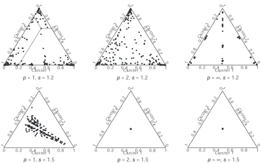
Figure 3: Triplot showing the cluster membership in F for each respondent for s= 1.2,1.5, λ= 1, and p= 1,2,∞.
showing fi2 of about .65. Finally, fi3 is obtained by projecting onto the axis
of Cluster 3 along a line parallel to Cluster 2, yielding fi3 of about .15. In
four decimals, these values are .2079, .6457, and .1464. Thus, a point located close to a corner implies that this respondent has almost solely assigned to this cluster. Also, a point exactly in the middle of the triangle implies an equal memberships of 1/3 to all three clusters. Finally, points that are on a straight line from a corner orthogonal to a cluster axis have equal cluster memberships of two clusters. For the case ofp=∞, Figure 3 shows a vertical line (starting in Cluster 2 and orthogonal to the Cluster 1 axis) implying that the memberships for Clusters 1 and 3 are the same for those respondents.
For the choice p = 2 and s = 1.5 and p = 2 or ∞, all clusters centers are in close proximity to each other in the center. In other words, all fuzzy memberships are about 1/3 and consequently the three cluster centers are the same. Therefore, s = 1.5 is too large for p = 2 or ∞. This finding is an indication of overlapping clusters. For a value of s = 1.2, the triplot for
p = 1 shows more pronounced clusters because most of the respondents are in the corners. For p = 2 and s = 1.2, the memberships are more evenly distributed over the triangle although many respondents are still located in the corners. Forp=∞ands= 1.2, some respondents are on the vertical line (combining equal memberships to Clusters 1 and 3 for varying membership of Cluster 2). The points that are located close to the Cluster 1 axis at .5 have a membership of .5 for Clusters 1 and 3, those close to .5 at the Cluster
0 0 0 0 .2 0.2 0.2 0 .4 0.4 0.4 0 .6 0.6 0.6 0 .8 0.8 0.8 1 1 1 Clus te r 1 C lu s te r 2 Clu ste r 3 0 0 0 0 .2 0.2 0.2 0 .4 0.4 0.4 0 .6 0.6 0.6 0 .8 0.8 0.8 1 1 1 Clus te r 1 C lu s te r 2 Clu ste r 3 0 0 0 0 .2 0.2 0.2 0 .4 0.4 0.4 0 .6 0.6 0.6 0 .8 0.8 0.8 1 1 1 Clus te r 1 C lu s te r 2 Clu ste r 3 p = 1, s = 1.2 p = 2, s = 1.2 p = ∞, s = 1.2 0 0 0 0 .2 0.2 0.2 0 .4 0.4 0.4 0 .6 0.6 0.6 0 .8 0.8 0.8 1 1 1 Clus te r 1 C lu ste r 2 Clu ste r 3 0 0 0 0 .2 0.2 0.2 0 .4 0.4 0.4 0 .6 0.6 0.6 0 .8 0.8 0.8 1 1 1 Clus te r 1 C lu ste r 2 Clu ste r 3 0 0 0 0 .2 0.2 0.2 0 .4 0.4 0.4 0 .6 0.6 0.6 0 .8 0.8 0.8 1 1 1 Clus te r 1 C lu ste r 2 Clu ste r 3 p = 1, s = 1.5 p = 2, s = 1.5 p = ∞, s = 1.5
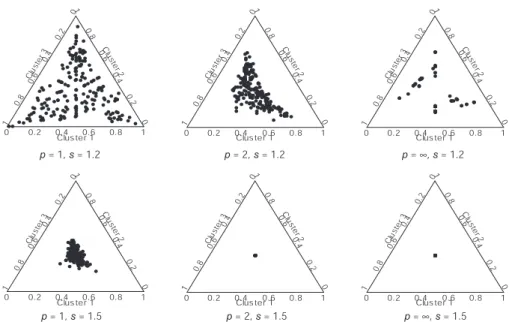
Figure 4: Triplot showing the cluster membership in F for each respondent for s= 1.2,1.5, λ=.5, and p= 1,2,∞..
2 axis have .5 for Clusters 1 and 2, those close to the Cluster 3 axis at .5 have .5 for Clusters 2 and 3.
For the robust case ofλ= 1/2, the triplots of the fuzzy memberships are given in Figure 4. One of the effects of setting λ= 1/2 seems to be that the
fikare more attracted to the center and, hence, respondents are less attracted
to a single cluster than in the case of λ = 1. Again, for s = 1.5 and p = 2 and ∞, all clusters merge into one cluster and the parallel coordinates plots of the clusters would show a single line. Fors = 1.2, the parallel coordinates plots of the clusters resemble Figure 2 reasonably well. For s = 1.2 and
p = 2, the lines in the parallel coordinates plot are closer together than for
λ = 1.
For this data set, the clusters cannot be well separated because for a relatively small s of 1.5, the clusters coincide (except forp= 1). The cluster centers seem to be better separated when p is small, especially for p = 1. The fuzziness parameter s needs to be chosen small in this data set to avoid clusters collapsing into a single cluster. The effect of varying λ seems to be that the cluster memberships are less extreme for λ= 1/2 than forλ= 1.
5
Conclusions
We have considered objective function based fuzzy clustering algorithms us-ing a generalized distance function. In particular, we have studied the exten-sion of the fuzzy c-means algorithm to the case of the parametric Minkowski distance function and to the case of the root of the squared Minkowski dis-tance function. We have derived the optimality conditions for the member-ship values from the Lagrangian function. For cluster centers, however, we have used iterative majorization to derive the optimality conditions. One of the advantages of iterative majorization is that it is a guaranteed descent algorithm, so that every iteration reduces the objective function until con-vergence is reached. We have derived suitable majorization functions for the distance function that we study. Extending results from Groenen and Jajuga (2001), we have given a majorization algorithm for any Minkowski distance with Minkowski parameter greater than (or equal to) 1. This extension also included the case of theL∞-distance and the roots of the squared Minkowski distance.
By adapting the Minkowski parameterp, the user influences the distance function to take specific cluster shapes into account. We have also introduced an additional parameterλfor computing the roots of the squared Minkowski distance. This parameter can be used to protect the clustering algorithm against outliers. Hence, more robust clustering results can be obtained.
We have illustrated some key aspects of the behaviour of our algorithm using empirical data regarding attitudes about the Internet. With this par-ticular data set, we have observed extremely overlapping clusters, already with a fuzziness parameter of s= 1.5. This finding deviates from the general practice in fuzzy clustering, where this parameter is often selected equal to 2. Apparently, the choice of s and p has to be done with some care for a given data set.
References
Babuˇska, R. (1998). Fuzzy modeling for control. Boston, MA: Kluwer Aca-demic Publishers.
Baraldi, A., & Blonda, P. (1999a, December). A survey of fuzzy clustering algorithms for pattern recognition — part I. IEEE Transactions on Systems, Man and Cybernetics, Part B, 29(6), 778–785.
Baraldi, A., & Blonda, P. (1999b, December). A survey of fuzzy clustering algorithms for pattern recognition — part I. IEEE Transactions on Systems, Man and Cybernetics, Part B, 29(6), 786–801.
Bezdek, J. C. (1973). Fuzzy mathematics in pattern classification. Unpub-lished doctoral dissertation, Cornell University, Ithaca.
Bezdek, J. C., Coray, C., Gunderson, R., & Watson, J. (1981a). Detection and characterization of cluster substructure, II. fuzzy c-varieties and convex combinations thereof. SIAM Journal of Applied Mathematics,
40(2), 358–372.
Bezdek, J. C., Coray, C., Gunderson, R., & Watson, J. (1981b). Detection and characterization of cluster substructure, I. linear structure: fuzzy c-lines. SIAM Journal of Applied Mathematics, 40(2), 339–357.
Bezdek, J. C., & Pal, S. K. (1992). Fuzzy models for pattern recognition. New York: IEEE Press.
Bobrowski, L., & Bezdek, J. C. (1991). c-Means clustering with the l1 and
l∞ norms. IEEE Transactions on Systems, Man, and Cybernetics, 21, 545–554.
Borg, I., & Groenen, P. J. F. (2005). Modern multidimensional scaling: Theory and applications (2nd ed.). New York: Springer.
Dave, R. N. (1991, November). Characterization and detection of noise in clustering. Pattern Recognition Letters,12(11), 657–664.
De Leeuw, J. (1994). Block relaxation algorithms in statistics. In H.-H. Bock, W. Lenski, & M. M. Richter (Eds.), Information systems and data analysis (pp. 308–324). Berlin: Springer.
Dodge, Y., & Rousson, V. (1998). Multivariate L1 mean. In A. Rizzi,
M. Vichi, & H. Bock (Eds.),Advances in data science and classification
(pp. 539–546). Berlin: Springer.
Dunn, J. (1973). A fuzzy relative of the isodata process and its use in de-tecting compact, well-separated clusters. Journal of Cybernetics,3(3), 32–57.
Groenen, P. J. F., & Heiser, W. J. (1996). The tunneling method for global optimization in multidimensional scaling. Psychometrika, 61, 529–550. Groenen, P. J. F., Heiser, W. J., & Meulman, J. J. (1999). Global optimiza-tion in least-squares multidimensional scaling by distance smoothing.
Journal of Classification, 16, 225–254.
Groenen, P. J. F., & Jajuga, K. (2001). Fuzzy clustering with squared Minkowski distances. Fuzzy Sets and Systems,120, 227–237.
Gustafson, D. E., & Kessel, W. C. (1979). Fuzzy clustering with a fuzzy covariance matrix. In Proc. ieee cdc (pp. 761–766). San Diego, USA. Hathaway, R. J., Bezdek, J. C., & Hu, Y. (2000, October). Generalized fuzzy
c–means clustering strategies using lp norm distances. IEEE
Transac-tions on Fuzzy Systems, 8(5), 576–582.
Heiser, W. J. (1995). Convergent computation by iterative majorization: Theory and applications in multidimensional data analysis. In W. J.
Krzanowski (Ed.), Recent advances in descriptive multivariate analysis
(pp. 157–189). Oxford: Oxford University Press.
H¨oppner, F., Klawonn, F., Kruse, R., & Runkler, T. (1999). Fuzzy cluster analysis: methods for classification, data analysis and image recogni-tion. New York: Wiley.
Hunter, D. R., & Lange, K. (2004). A tutorial on MM algorithms. The American Statistician, 39, 30–37.
Inselberg, A. (1981). N-dimensional graphics, part I: Lines and hyperplanes
(Tech. Rep. No. G320-2711). Los Angeles (CA): IBM Los Angeles Scientific Center.
Inselberg, A. (1997). Multidimensional detective. In Proc. ieee symp. infor-mation visualization (p. 100-107).
Jajuga, K. (1991). L1-norm based fuzzy clustering. Fuzzy Sets and Systems,
39, 43–50.
Kaymak, U., & Setnes, M. (2002, December). Fuzzy clustering with volume prototypes and adaptive cluster merging. IEEE Transactions on Fuzzy Systems, 10(6), 705–712.
Kiers, H. A. L. (2002). Setting up alternating least squares and iterative ma-jorization algorithms for solving various matrix optimization problems.
Computational Statistics and Data Analysis, 41, 157–170.
Lange, K., Hunter, D. R., & Yang, I. (2000). Optimization transfer using surrogate objective functions. Journal of Computational and Graphical Statistics,9, 1–20.
Ruspini, E. (1969). A new approach to clustering. Information and Control,
15, 22–32.
Yang, M.-S. (1993). A survey of fuzzy clustering. Mathematical and Com-puter Modelling, 18(11), 1–16.
![Figure 1: The original function d 2 (t) and the majorizing functions for p = 1, p = 3, and p = ∞ using supporting point u = [2, −3] 0 .](https://thumb-us.123doks.com/thumbv2/123dok_us/1444888.2693418/12.892.310.575.285.934/figure-original-function-majorizing-functions-using-supporting-point.webp)