Reflecting Human Knowledge of Place and Route-Choice Behavior Using Big Data

(1)

University of Tennessee, Knoxville

Trace: Tennessee Research and Creative

Exchange

Doctoral Dissertations Graduate School

5-2017

Reflecting Human Knowledge of Place and

Route-Choice Behavior Using Big Data

Jiaoli Chen

University of Tennessee, Knoxville, [email protected]

This Dissertation is brought to you for free and open access by the Graduate School at Trace: Tennessee Research and Creative Exchange. It has been accepted for inclusion in Doctoral Dissertations by an authorized administrator of Trace: Tennessee Research and Creative Exchange. For more information, please [email protected].

Recommended Citation

Chen, Jiaoli, "Reflecting Human Knowledge of Place and Route-Choice Behavior Using Big Data. " PhD diss., University of Tennessee, 2017.

(2)

To the Graduate Council:

I am submitting herewith a dissertation written by Jiaoli Chen entitled "Reflecting Human Knowledge of Place and Route-Choice Behavior Using Big Data." I have examined the final electronic copy of this dissertation for form and content and recommend that it be accepted in partial fulfillment of the requirements for the degree of Doctor of Philosophy, with a major in Geography.

Shih-Lung Shaw, Major Professor We have read this dissertation and recommend its acceptance:

Bruce A. Ralston, Hyun Kim, Lee D. Han

Accepted for the Council: Dixie L. Thompson Vice Provost and Dean of the Graduate School (Original signatures are on file with official student records.)

(3)

Reflecting Human Knowledge of Place and

Route-Choice Behavior Using Big Data

A Dissertation Presented for the

Doctor of Philosophy

Degree

The University of Tennessee, Knoxville

Jiaoli Chen

May 2017

(4)

(5)

iii

DEDICATION

I dedicate this dissertation to my parents, Huiyu Chen and Xiangping Li, who are always doing their best to love and support me. This dissertation is also dedicated to my fiancé, Ye Hao, who took care of me during my PhD research.

(6)

iv

ACKNOWLEDGEMENTS

I am very grateful to my advisor, Dr. Shih-Lung Shaw. Dr. Shaw encouraged me to gain confidence in everything. It is a great wealth for both my career and life. His academic advice and support helped me get abilities of critical thinking and independent research. He also helped me realize the importance of real-world thinking. This is the biggest gain during my Ph.D. period and will definitely benefit my future career.

Many thanks to Dr. Bruce Ralston. From Dr. Ralston I have learnt the importance of keeping learning new things. He showed me what an active person should be like. He is always happy to share new technologies with students and willing to provide help.

I am very thankful to Dr. Hyun Kim and Dr. Lee Han. Dr. Kim is such a nice teacher and gave me many detailed suggestions for both course work and dissertation. Dr. Han also provided many useful suggestions for my dissertation research.

(7)

v

ABSTRACT

Exploring human knowledge of geographical space and related behavior not only helps in understanding human-environment interactions and dynamic geographic processes, but also advances Geographic Information Systems (GIS) toward a human-centric paradigm to make daily life more efficient. Today’s relatively easy acquisition of various big data provides an unprecedented opportunity for geographers to answer research questions that previously could not be adequately addressed. However, new challenges also arise regarding data quality and bias as well as change in methodology for dealing with big data that are different from traditional data types.

Representing people’s perception of place and studying driver’s route-choice behavior are two of the many applications of big data in answering research questions about human knowledge and behavior in the fields of GIS and transportation. Incorporating three papers, this dissertation focuses on these two different applications to achieve the following objectives: 1) examine the degree to which a geographic place’s spatial extent can be estimated from human-generated geotagged photos; 2) address the challenge of geotagged photos’ uneven spatial distribution in place estimation and explore an approach that can better derive a place’s spatial extent; 3) develop a method that can properly estimate the spatial extent of a place that has multiple disjoint regions while considering geotagged photos’ uneven distribution; 4) explore useful spatiotemporal patterns of taxi drivers’ route-choice behavior in a dynamic urban environment.

This dissertation makes three major contributions to big data applications’ systematic theory: 1) proposes an effective approach to handling the uneven spatial distribution problem of geotagged photos as a type of volunteered geographic data by modeling their representativeness; 2) develops methods that can properly derive the vague spatial extent of a place with or without disjoint regions; and 3) explores taxi drivers’ route-choice patterns in different situations that can inform future transportation decisions and policy-making processes.

(8)

vi

LIST OF TABLES

Table 3.1 Performance comparison of determining disjoint extents under different significance levels. (The number with * indicates that among the detected significant clusters, there are two clusters corresponding to one place extent.)

... 45

Table 3.2 Accuracy comparison of outlier removal in local area. ... 48

Table 4.1 Functional classification of Wuhan road network. ... 63

Table 4.2 Categories of NonSDR ratios and Categories of NonGTR ratios. ... 69

(11)

ix

LIST OF FIGURES

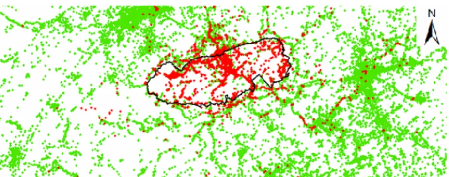
Figure 2.1 Spatial distributions of target points (red) and all points (red and green) of the Great Smoky Mountains National Park. The official boundary is shown in black solid line. ... 18 Figure 2.2 DTC with the target points (red dots) of Nashville: (a) edges connecting

neighbors constructed by Delaunay Triangulation; (b) resulting major cluster with its convex hull (in dash line). (c) Flow chart of the search procedure for cut-off distance c. ... 19 Figure 2.3 Vague spatial extents represented by KDE (top row of each place) vs.

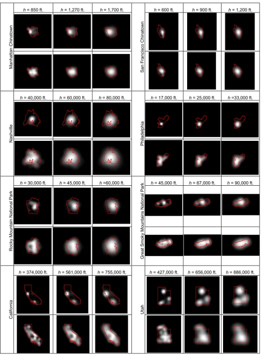
RW-KDE surfaces (bottom row) under different bandwidths (h). Reference boundaries are in red line. ... 22 Figure 2.4 In each pair of (a) to (c), (left) a popularity density surface based on all

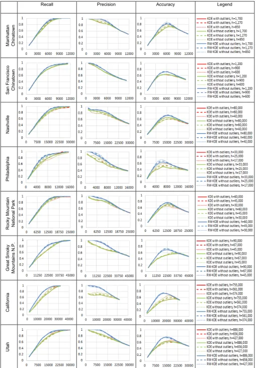
Flickr photos using KDE; (right) a scatter plot of the estimates from the resulting KDE and RW-KDE surfaces against the popularity densities within the official boundary of California. ... 23 Figure 2.5 Recall, precision, and accuracy of the boundaries derived from the KDE

and RW-KDE surfaces. The x axis represents the rank threshold β used to derive crisp boundary. The y axis in the second, third, and fourth columns represent the recall, precision, and accuracy measures, respectively. ... 25 Figure 3.1 Search results of Chinatown, New York City from (a) Google Maps and

(b) Wikipedia. ... 34 Figure 3.2 Spatial distribution of the Flickr photos tagged with “Chinatown” in New

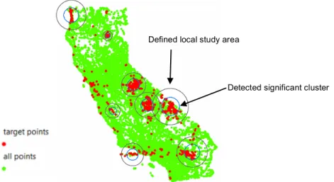
York City. ... 37 Figure 3.3 Examples of circular windows (blue circles) centered on the target

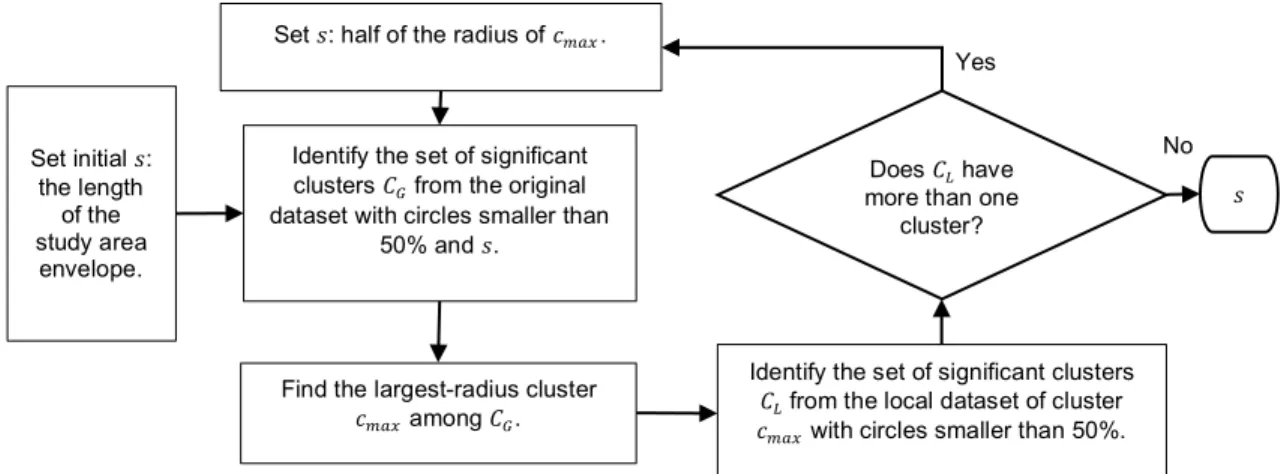
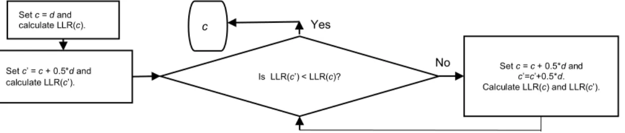
points tagged with “national park” (red dots). The green dots represent the set of all points in California. ... 39 Figure 3.4 Search procedure for the maximum circle size. ... 41 Figure 3.5 Example of the local study areas (black circles) centered on the

detected clusters (blue circles) of target points in California. ... 42 Figure 3.6 Search procedure for threshold distance c. ... 43 Figure 3.7 Detected significant clusters (blue circles) of disjoint extents at α=0.001

vs. reference boundaries of (a) National Park, (b) Square Park and (c) Chinatown. Grey dots are photo points with a target place name. Reference boundaries are in red lines, which applies to all following figures. ... 46 Figure 3.8 Results of outlier removal based on the highest LLR approach in local

study areas. Green dots are valid points after outlier removal. Grey dots are outliers to be removed. ... 49 Figure 3.9 Examples of improved outlier removal results. Left: HLLR-based outlier

removal. Right: original RW-KDE outlier removal. ... 50 Figure 3.10 RW-KDE-FDE surfaces of (a) National Park, (b) Chinatown, and (c)

(12)

x

Figure 3.11 Density surface comparison of Chinatown: (a) traditional KDE, (b) RW-KDE based on global study area, and (c) RW-RW-KDE-FDE based on local study area. ... 52 Figure 4.1 Spatial distributions of six functional classes of Wuhan road network. ... 64 Figure 4.2 Three scenarios for one road segment (from junction A to junction B)

related to three different taxi trips (O1 to D1, O2 to D2 and O3 to D3): (a) Matched road segment, (b) NonSDR road segment, and (c) NonGTR road segment. ... 66 Figure 4.3 Temporal distributions of (a) NonSDR ratios and (b) NonGTR ratios of

the road segments selected as examples from each category. ... 70 Figure 4.4 Spatial distributions of the four categories of NonSDR ratios. ... 71 Figure 4.5 Spatial distributions of the four categories of NonGTR ratios. ... 72 Figure 4.6 Comparison of functional class composition among different categories. ... 74 Figure 4.7 Travel distance and road class preference (x axis: travel distance

interval in km; y axis: difference of a functional class’ share in the actual routes vs. in the shortest-distance routes). ... 77 Figure 4.8 Temporal variation of city roads’ average speed. ... 79 Figure 4.9 (a-d) Non-SDR ratio’s spatial distribution in four situations. (e-h) Roads

with a noticeable difference in the Non-SDR ratio between (a) and (b), (c) and (d), (a) and (c), (b) and (d). ... 80 Figure 4.10 (a-d) Non-GTR ratio’s spatial distribution in four situations. (e-h) Roads

with a noticeable difference in the Non-GTR ratio between (a) and (b), (c) and (d), (a) and (c), (b) and (d). ... 81 Figure 4.11 Cumulative distribution of (a1-a5) SDR ratios and (b1-b5) Non-GTR ratios in the road classes of (a1,b1) state road; (a2, b2) city expressway; (a3, b3) urban major arterial; (a4, b4) urban minor arterial; and (a5, b5) local street, by different situations. ... 83 Figure 4.12 Distribution of (a1-a4) Non-SDR ratios and (b1-b4) Non-GTR ratios in

different road classes in the following situations: (a1, b1) long trip in rush hours; (a2, b2) long trip in off-rush hours; (a3, b3) short trip in rush hours; (a4, b4) short trip in off-rush hours. ... 84

(13)

1

Chapter 1 Introduction

(14)

2

1.1 Research Background

Human perception and knowledge of geographical space are often formed during people’s interactions with environments by conducting various daily activities (Tuan 1977, Massey 1994). In turn, perception and knowledge influence human daily practice, such as inhabiting, traveling, communicating and working, which are the underlying contributors to human and urban dynamics. Acquiring information about human knowledge and behavior is important in studying such fields as Geographic Information System/Science (GIS) and transportation. This information can be used to achieve the following research goals: explaining geographic reality and process (Goodchild 2011), understanding human and urban dynamics, developing human-centric GIS tools and services, providing smarter navigation applications, mitigating urban traffic congestions, and designing efficient transportation and urban systems.

People’s perception and knowledge of geographical space and related behavior are also revealed in a wide range of informal ways (e.g., use of place names to refer to geographic locations, use of words and sentences to describe one’s feeling about and experience of the surroundings, pictures and videos of interest, and trajectories of one’s route-choice decisions). Before the age of ubiquitous information and communications technology (ICT), data about such perception, knowledge and behavior was acquired through interviews, surveys and experiments. This kind of data collection is tedious, time-consuming and expensive. Furthermore, the data generally have low coverage of space and time, reflect a small proportion of the population, and are usually static. The challenge of obtaining large-scale datasets containing information about human perception and behavior once prevented researchers from answering interesting research questions about human dynamics.

In contrast, today’s pervasive information and communication devices (e.g., computers, mobile phones, global positioning system (GPS), cameras and radio-frequency identification) record and track human discourses and activities with high spatial and temporal resolutions. The big data created in the digital world are now regarded to be valuable “exaflood” (Swanson 2007) in both business and scientific worlds (Sui et al. 2013). The GIS community has used those geographically related big data from different sources to address various geographic and transportation topics.

Different data types have varying degrees of suitability for examining different perspectives of human perception, knowledge and behavior. The major categories of most used geographically and/or temporally referenced big data and the related research topics regarding human perception, knowledge and behavior include the following:

(15)

3

1. Georeferenced social media data as sensors of geographic space’s social content. These data are created by ordinary citizens during their participation in online social media, such as geotagged Flickr photos and tags, Twitter tweets, Facebook postings and Foursquare check-ins. Closer to human discourse than other data types containing only geolocations, they are often used to examine geographic space’s social side, such as harvesting human perception of a place (e.g., Gao et al. 2014) and inferring social characteristics about physical space (e.g., Graham and Zook 2011, McKenzie et al. 2015). Researchers also use these data to explore human behavior and activity patterns (e.g., Azmandian et al. 2013, Hasan et al. 2013).

2. Tracking data collected from GPS devices. These trajectory data have been applied to explore and understand the spatiotemporal patterns of human activity-travel behavior as well as resulting human and urban dynamics, such as dynamic urban flows (e.g., Giannotti et al. 2011, Veloso et al. 2011), city hotspot extraction (e.g., Palma et al. 2008), collective human mobility (e.g., Liu et al. 2012, Jiang et al. 2009), time-varying traffic condition (Ehmke et al. 2012), and routing-strategy differences between drivers (Liu et al. 2010).

3. Location data collected from mobile phone devices that are more pervasive provide individual persons’ digital footprints. The unit of cell phone data (individual person) is “finer” (i.e., more direct human footprint at the individual level) than that of vehicle GPS tracking data (vehicle). Thus, such data are frequently used to study human-activity space (Yuan et al. 2012, Xu et al. 2016) and mobility patterns (González et al. 2008).

These big data bring not only opportunities for studying human dynamics but also new challenges when dealing with the issues caused by the three V’s of big data: volume, velocity and variety (Laney 2001). Thus, new methods and tools are needed to increase capabilities to process, analyze and visualize such new type of data (Sui and Goodchild 2011). Miller and Goodchild (2015) suggest that in data-driven science, GIS methods and tools should shift from finding explanations and universal laws to exploring specific patterns and descriptions at certain places and times. Methods should also be specifically developed for certain data types and research questions.

Addressing specific opportunities and challenges for different types of big data and research questions, this dissertation focuses on two of the many perspectives in big data applications: reflecting human perception of place and understanding route-choice behavior. The concepts of place and route-choice behavior play important roles in human dynamics and are examined in this dissertation on the scope of human dynamics. Human perception of place (e.g., home, work place, business place and commercial place) greatly influences urban system and travel demands, which are directly related to human dynamics in a city. Route-choice

(16)

4

decisions between two places can both influence and be influenced by time-varying flows in urban dynamics. More details regarding specific research questions are discussed in the following subsections.

1.1.1 Reflecting Human Perception of Place Using Geotagged Photos

The concept of place comes from associating social meanings to physical space through human interactions and experiences with geographic environments (Tuan 1977, Agnew 2011). This concept is common in human discourse (e.g., using place names in daily conversations to specify locations). People often ask such questions as “where is Chinatown in New York City,” but its extent usually cannot be located on a map. Chinatown is a vernacular name coming from people’s understanding of a neighborhood’s social characteristics but has not been officially defined by authorities. Thus, it is a vague concept in terms of undefined geographic boundary and varying perceptions among people. GIS tools and services need to better represent place from a spatial perspective to bridge informal human discourse and a precise computational environment.

Human perception and knowledge of a place are difficult to identify until they are explicitly expressed. During the past decade, GIS and social media have been converging (Sui and Goodchild 2011). For example, most social media websites provide a location-sharing function enabling users to assign a geolocation to their postings (e.g., Twitter tweets, Facebook status updates, and Flickr photos). From the geographic perspective, this geotagging is a process in which people explicitly express their ideas about a location based on their experience, knowledge, understanding and feeling. Among the geotagged textual contents, place names are included and their relationship to corresponding geolocations are established. Thus, a place’s spatial extent can be estimated using the geolocations that social media users consider to be inside the place.

The convergence of GIS and social media has brought an era of humans as sensors (Goodchild 2007) in which a bottom-up crowdsourcing process of average citizens’ geographic data production is emerging to supplement the traditional top-down authoritative process of geographic data production (Sui et al. 2013). This approach promotes interest in researching human knowledge of place based on volunteered geographic data that are unprecedentedly large scale and dynamic. However, the three V’s issues associated with big data also exist in volunteered geographic information (VGI) (Goodchild et al. 2016), and new methodologies are needed. Specifically, when such VGI is used to reflect human perception and knowledge of place, challenges exist in terms of systematically biased representation in user groups and spatial coverage (Lüscher and Weibel 2013, Hollenstein and Purves 2010) as well as lack of quality assurance (Goodchild and Li 2012). In other words, social media users who contribute to the VGI content may not represent the perception and knowledge of people who do not use social media.

(17)

5

Moreover, geotagged content’s availability and distribution are inconsistent over the entire geographic space. For example, less or no content is available in unpopular areas. Furthermore, VGI’s contributors are average citizens who might not be well trained with geographic knowledge. They tend to make mistakes and reduce VGI’s quality.

Given the above challenges in using human-generated content conveying information about human perception and knowledge of a place to explicitly represent and visualize such information, this dissertation aims to address the following research questions:

To what degree can biased representation and no quality assurance influence the estimation of place extents based on geotagged photos? Can these problems be overcome? What are some effective approaches to overcoming them?

How effective are the geotagged photos for deriving vague spatial extents of places? To what degree can these extents be correctly approximated?

1.1.2 Exploring Spatiotemporal Patterns of Route-Choice Behavior Using GPS Tracking Data

Reflecting human perception and knowledge of place discussed in Subsection 1.1.1 advances GIS tools and services toward a human-centric paradigm by helping answer a real-world question about a place’s location. Acquiring route-choice behavior’s spatiotemporal patterns can also help improve GIS services’ performance in navigation applications by answering a real-world question about what is a good route between two places.

The mutual influence between human route-choice behavior and a transportation system is one of urban dynamics’ major components. Route-choice decisions are made under various constraints, such as space and time, and can influence the level of human mobility. Development of transportation systems depends heavily on the characteristics of urban residents’ activity-travel behaviors, which include route-choice behavior. After Hägerstrand (1970) initiated the era of time geography, transportation research’s focus changed from conventional trip-based aggregate approaches to activity-based disaggregate approaches under space-time constraints (Timmermans et al. 2002). This focus requires more detailed information about route-choice behavior at the individual level and under different space-time situations. The commonly used assumption of optimal route could be no longer applicable if urban dynamics and human factors are considered (Li et al. 2011). Although the literature shows great efforts in examining the factors influencing route-choice decisions (e.g., Hölscher et al. 2011, Papinski et al. 2009),

(18)

6

route-choice behavior’s dynamic property and spatial variation have not often been considered.

A city’s taxi GPS tracking data include detailed information about which routes taxi drivers chose and what strategies were used to avoid bad traffic conditions (Castro et al. 2013). This large dataset can help explore spatiotemporal patterns of route-choice behavior and validate conclusions from existing studies. However, mining such big trajectory data involves some challenges: large data size, multiple dimensions, and coexistence of homogeneity and heterogeneity in human behavior patterns. Existing data-mining and knowledge-discovery approaches have difficulty dealing with space-time constraints in human movements. These challenges call for higher computational power and innovative spatiotemporal data-mining approaches while simultaneously considering space and time. Thus, this dissertation focuses on developing effective and efficient space-time approaches to exploring spatiotemporal patterns of taxi drivers’ route-choice behavior considering urban dynamics. Specific research questions include the following:

Where, when, and to what extent do taxi drivers deviate from the shortest-distance routes? What are some effective methods for facilitating spatiotemporal analysis of taxi drivers’ deviation patterns? Are road functional class, travel distance and urban rush hours related to taxi drivers’ deviations from the shortest-distance routes? Which factors are more influential? What unknown patterns can be found from big taxi tracking data? Are the conclusions drawn from such big data consistent with those from traditional survey and sample data?

1.2 Organization of Chapters

The remainder of this dissertation consists of three paper chapters plus one concluding chapter. Each paper chapter is written in the form of journal article. Chapters 2 and 3 answer the research questions listed in Subsection 1.1.1 from the perspective of human perception and knowledge of place. Chapter 4 answers the research questions in Subsection 1.1.2 from the perspective of human route-choice behavior. These three chapters are organized as three independent papers. Chapter 2 explores the important impact of geotagged photos’ uneven spatial distribution on estimating vague place extents. To overcome the biased spatial coverage, an approach is proposed for modeling the representativeness of each geotagged photo point based on its location popularity. A modified kernel density estimation method incorporating photo representativeness is developed. It is tested with eight places, which cover urban vs. non-urban areas, with vs. without

(19)

7

an official boundary cases, and at various spatial scales of state, city and district levels. The test results indicate noticeable improvements of the proposed representativeness-weighted kernel density estimation (RW-KDE) method over the traditional kernel density estimation method in estimating places’ vague spatial extent. The results also indicate that using geotagged photos is feasible to derive acceptable spatial extent of places once the unevenly distributed photos’ representativeness is properly adjusted.

Chapter 3 identifies a challenge caused by outlier photos (i.e., photos tagged with a target place name but not located within the target place) when using geotagged photos to estimate the spatial extent of a place with multiple disjoint extents located in different regions of a large study area. This chapter proposes a method named

representativeness-weighted kernel density estimation for disjoint extents (RW-KDE-FDE). This method first uses a scan statistic approach to determine the number and rough locations of a place’s disjoint extents, and then applies an improved outlier-removal process and RW-KDE approach to derive the vague extents. The method is tested with three places that have disjoint extents in study areas of different scales. The results show a place’s disjoint extents and their improved spatial representation.

Chapter 4 focuses on taxi drivers’ route-choice patterns at different locations and times and in different situations by comparing their actual routes to the shortest-distance routes. Two indices measuring taxi drivers’ preference for and avoidance of each road segment are proposed to help reveal the spatiotemporal patterns of taxi drivers’ deviations from the shortest-distance routes. This chapter finds that deviation from the shortest-distance route is influenced more by road functional class and travel distance than by urban rush hours. Taxi drivers tend to frequently detour from the shortest-distance routes in areas with a high density of local streets, but tend to follow the shortest-distance routes on high-hierarchy roads and short trips. Taxi drivers are not likely to choose a primary road as an alternative if it is not on the distance route, but once a primary road is on the shortest-distance route, they tend to stay on it. By examining the difference in deviation rate between rush hours and off-rush hours, this chapter finds that the aggregate patterns of taxi drivers’ deviations are relatively stable regardless of urban rush hours.

Chapter 5 summarizes this dissertation research’s major contributions and identifies limitations as well as future research directions.

(20)

8

References

Agnew, J.A., 2011. Space and place. In: J.A. Agnew and D.N. Livingstone, eds.

The SAGE handbook of geographical knowledge. Thousand Oaks, CA: SAGE, 316–330.

Azmandian, M., et al., 2013. Following human mobility using tweets. In: L. Cao, et al., eds. Agents and data mining interaction. ADMI 2012. Lecture notes in computer science vol. 7607. Berlin: Springer, 139-149.

Ehmke, J. F., Meisel, S., and Mattfeld, D. C., 2012. Floating car based travel times for city logistics. Transportation Research Part C: Emerging Technologies, 21(1), 338-352.

Gao, S., et al., 2014. Constructing gazetteers from volunteered big geo-data based on Hadoop. Computers, Environment and Urban Systems.

Castro, P. S., et al., 2013. From taxi GPS traces to social and community dynamics.

ACM Computing Surveys, 46(2), 1-34.

González, M.C., Hidalgo, C.A., and Barabási, A.L., 2008. Understanding individual human mobility patterns. Nature, 453(7196), 779–782.

Goodchild, M.F., 2007. Citizens as sensors: the world of volunteered geography.

GeoJournal, 69(4), 211-221.

Goodchild, M.F., 2011. Formalizing place in geographic information systems. In: L.M. Burton, et al., eds. Communities, neighborhoods, and health. New York: Springer, 21-33.

Goodchild, M.F., Aubrecht, C., and Bhaduri, B., 2016. New questions and a changing focus in advanced VGI research. Transactions in GIS, 1-2.

Goodchild, M.F. and Li, L., 2012. Assuring the quality of volunteered geographic information. Spatial Statistics, 1, 110-120.

Giannotti, F., et al., 2011. Unveiling the complexity of human mobility by querying and mining massive trajectory data. The VLDB Journal—the International Journal on Very Large Data Bases, 20(5), 695-719.

Hägerstrand, T., 1970. What about people in regional science? Papers in Regional Science, 24(1), 7-24.

Hasan, S., Zhan, X., and Ukkusuri, S.V., 2013. Understanding urban human activity and mobility patterns using large-scale location-based data from online social media. In: Proceedings of the 2nd ACM SIGKDD international workshop on urban computing. New York: ACM.

Hollenstein, L. and Purves, R., 2010. Exploring place through user-generated content: using Flickr tags to describe city cores. Journal of Spatial Information Science, 1, 21-48.

Li, Q., et al., 2011. Path-finding through flexible hierarchical road networks: An experiential approach using taxi trajectory data. International Journal of Applied Earth Observation and Geoinformation, 13(1), 110-119.

Hölscher, C., Tenbrink, T., and Wiener, J. M, 2011. Would you follow your own route description? Cognitive strategies in urban route planning. Cognition, 121(2), 228-247.

(21)

9

Lüscher, P. and Weibel, R., 2013. Exploiting empirical knowledge for automatic delineation of city centres from large-scale topographic databases.

Computers, Environment and Urban Systems, 37, 18-34.

Massey, D., 1994. Space, place and gender. Cambridge: Polity Press.

McKenzie, G., et al., 2015. How where is when? On the regional variability and resolution of geosocial temporal signatures for points of interest. Computers, Environment and Urban Systems, 54, 336-346.

Miller, H.J. and Goodchild, M.F., 2015. Data-driven geography. GeoJournal, 80(4), 449-461.

Graham, M. and Zook, M., 2011. Visualizing global cyberscapes: Mapping user-generated placemarks. Journal of Urban Technology, 18(1), 115-132. Jiang, B., Yin, J., and Zhao, S., 2009. Characterizing the human mobility pattern

in a large street network. Physical Review E, 80(2), 021136.

Laney, D., 2001. 3D data management: Controlling data volume, velocity, and variety. META Group. Available from: http://blogs.gartner.com/doug-

laney/files/2012/01/ad949-3D-Data-Management-Controlling-Data-Volume-Velocity-and-Variety.pdf [Accessed November 1, 2016].

Liu, L., Andris, C., and Ratti, C., 2010. Uncovering cabdrivers’ behavior patterns from their digital traces. Computers, Environment and Urban Systems, 34(6), 541-548.

Liu, Y., et al., 2012. Understanding intra-urban trip patterns from taxi trajectory data. Journal of Geographical Systems, 14(4), 463-483.

Palma, A. T., et al., 2008. A clustering-based approach for discovering interesting places in trajectories. In: Proceedings of the 2008 ACM symposium on applied computing. New York: ACM, 863-868.

Papinski, D., Scott, D. M., and Doherty, S. T., 2009. Exploring the route choice decision-making process: A comparison of planned and observed routes obtained using person-based GPS. Transportation Research Part F: Traffic Psychology and Behaviour, 12(4), 347-358.

Sui, D. and Goodchild, M., 2011. The convergence of GIS and social media: challenges for GIScience. International Journal of Geographical Information Science, 25(11), 1737-1748.

Sui, D., Goodchild, M., and Elwood, S., 2013. Volunteered geographic information, the exaflood, and the growing digital divide. In: D. Sui, S. Elwood, and M. Goodchild, eds. Crowdsourcing geographic knowledge. Netherlands: Springer, 1-12.

Swanson, B., 2007. The coming exaflood. The Wall Street Journal. Available from: http://www.wsj.com/articles/SB116925820512582318 [Accessed October 15, 2016].

Tuan, Y.F., 1977. Space and place: the perspective of experience. Minneapolis: Uiversity of Minnesota Press.

Veloso, M., Phithakkitnukoon, S., and Bento, C., 2011. Urban mobility study using taxi traces. In: Proceedings of the 2011 international workshop on trajectory data mining and analysis. New York: ACM, 23-30.

(22)

10 Timmermans, H., Arentze, T., and Joh, C.H., 2002. Analysing space-time behaviour: new approaches to old problems. Progress in Human Geography, 26(2), 175-190.

Xu, Y., et al., 2016. Another tale of two cities: understanding human activity space using actively tracked cellphone location data. Annals of the American Association of Geographers, 106(2), 489-502.

Yuan Y, Raubal, M., and Liu, Y., 2012. Correlating mobile phone usage and travel behavior - A case study of Harbin, China. Computers, Environment and Urban Systems, 36(2), 118–130.

(23)

11

Chapter 2 Representing the Spatial Extent of Places Based on Flickr

Photos with a Representativeness-Weighted Kernel Density

(24)

12 This chapter has been published as: Chen, J. and Shaw, S.L., 2016. Representing the spatial extent of places based on Flickr photos with a representativeness-weighted kernel density estimation. In: J.A. Miller, D. O’Sullivan, and N. Wiegand, eds. Geographic Information Science. Lecture notes in computer science vol. 9927. Cham: Springer, 130-144.

The research work was completed by Jiaoli Chen advised by Dr. Shih-Lung Shaw.

Abstract

Geotagged photos have been applied by many researchers to explore the spatial extent of places. This paper addresses an important challenge of using geotagged Flickr photos to delineate the spatial extent of a vague place, which is defined as a place without a clearly defined boundary. We argue that the variation of location popularity has a great impact on the estimation of such vague spatial extent of a place. We propose an approach to model the representativeness of each geotagged photo point based on its location popularity. A modified kernel density estimation method incorporating the photo representativeness is developed and tested with eight places, which cover urban vs. non-urban areas, with vs. without an official boundary cases, and at various spatial scales of state, city and district levels. Our results indicate major improvements of the proposed representativeness-weighted kernel density estimation method over the traditional kernel density estimation method in estimating the spatial extent of vague places.

2.1 Introduction

Naïve geography (Egenhofer and Mark 1995) envisions that the advanced geographic information systems (GIS) should “follow human intuition” (p. 1) and “support common-sense reasoning” (p. 5) so that ordinary people who do not need to know about GIS can use them easily. It is important for such GIS to understand and represent linguistic place names. Some places (e.g., administrative divisions) have a formally defined geographic extent to be represented in GIS, while many places (e.g., vernacular places) have no formally defined boundary but a vague geographic extent. Therefore, an effective and efficient representation of vague spatial extent of places is critical to GIS representation, query, analysis, and visualization of places.

Acquiring human knowledge of places is a traditional way to derive vague place extents. With the increasing popularity of geotagged social media (e.g., Flickr, Twitter, and Facebook), large numbers of place names exist in the contents from such platforms, carrying valuable information about people’s perception of places. Among these social media, Flickr provides adequate and more direct associations between photo geolocations and place name tags (Martins 2011). Thus, extracting the spatial extent of places from Flickr data has been a GIS research topic (e.g.,

(25)

13 Grothe and Schaab 2009, Hollenstein and Purves 2010, Li and Goodchild 2012, Cunha and Martins 2014), especially for purposes of enriching large-scale gazetteers and GIS services (e.g., Keßler et al. 2009a, Gao et al. 2014). In the meantime, such crowd-sourced data also present challenges to place-related research, including to which degree the spatial extent of a place can be estimated from geotagged photos or other crowd-sourced social media data.

Past research has indicated the effectiveness of using Flickr data to identify major locations of vague places (e.g., Hollenstein and Purves 2010, Keßler et al. 2009b). However, estimation of vague geographic extents still presents a major challenge. As suggested by Jones et al. (2008), we argue that the underlying assumption of a random distribution of Flicker photos is incorrect when applying geotagged photos to estimate vague place extents. In general, there are fewer photos taken at locations with low accessibility and low popularity than those popular and easily accessible locations. The conventional approach of treating each geotagged photo with equal representativeness or importance, regardless of where it is located, is questionable. The representativeness of photo points located in unpopular areas could be under-weighted due to a low absolute number of photos taken in such areas, while the representativeness of photo points located in popular areas would be over-weighted due to a larger number of photos taken in these areas. As a result, unpopular locations (e.g., inaccessible parts of mountain areas) of a vague place (e.g., Rocky Mountains) would be significantly underestimated or even excluded in the derived geographic extent. On the other hand, popular locations could be overestimated and distort the boundary of a place. When the kernel density estimation (KDE) method is applied to delineate vague boundaries (e.g., Li and Goodchild 2012), the resulting surface usually looks like a hot spot map of the photos tagged with a target place name rather than a “probability field” (p. 205) (Goodchild et al. 1998) representing the place extent where a higher estimate indicates a higher probability of belonging to a target place. Thus, this study aims at improving the representation of vague place extents by adjusting photo point representativeness based on their location popularity. Note that we adopt the same term “target place” (p.1047) from Jones et al. (2008) to refer to a place whose extent needs to be estimated.

In the remainder of this paper, we start with a review of work related to the concept of place, georeferencing place names, and delineation of vague place extent from survey, web and social media data. In the methodology part, we discuss a proposed approach based on photo point representativeness and the representativeness-weighted KDE (RW-KDE) method. Next, we present the results of testing our proposed assumptions and method based on eight selected sample places, followed by comparisons with the results derived from the traditional KDE approach. We conclude this paper with contributions, limitations and future research directions.

(26)

14

2.2 Related Work

As an important concept in geography, place has been extensively studied, implying more than space by incorporating social, economic, cultural and political meanings through human experience (Relph 1976, Tuan 1977, Agnew 2011). Places are usually revealed in unstructured forms. Their informality is also reflected by the variations in people’s understanding of them (Twaroch et al. 2009). Thus, they are often absent from current GIS in which geographic objects need to be disambiguated, abstracted and digitalized from the perspective of space. Great efforts have been made toward the convergence of place and GIS, such as theoretically modeling place in a computational environment (e.g., Cohn and Gotts 1996, Dilo et al. 2007) and delineating the spatial extent of place names which is the focus of this paper.

There have been some place-friendly web applications using simple gazetteers to handle place names (Jones et al. 2008). But retrieval of vague place extent is still beyond the ability of current gazetteers. Usually given an authority-recognized place name, a gazetteer provides information about its geographic location, feature type, and relationship to other places (Goodchild and Hill 2008). But it provides limited information on vernacular names. In most gazetteers, the location of a place with a large spatial extent is usually represented as a point, rectangle bounding box, or occasionally a polygon with crisp boundary (Twaroch et al. 2009). Although an abstract and simple geometry benefits computational process in current information systems, it falls short in delivering information about the inherent vagueness of place boundary which often reflects human perception and cognition. Therefore, much research has focused on deriving vague place extents from a variety of data sources.

Montello et al. (2003) conducted an empirical study in which human subjects were asked to draw shapes of the downtown Santa Barbara area based on their understanding of the place extent. The downtown shapes drawn by different participants were then aggregated to generate a probabilistic representation of the vague place extent. Montello et al. (2014) interviewed another two groups of participants to unveil and measure the variation of vagueness of a place perceived by different people and at different locations. These survey-based approaches have an advantage that data structure and collection procedure can be designed to facilitate subsequent modeling and estimation of vague place extents as well as to answer specific research questions. However, the difficulty in collecting such empirical data obstructs their wide applications.

Some other research derived a place’s extent using its topological relations to other clearly defined geographic objects. Based on a set of points covering a region, Parker and Downs (2013) combined DBSCAN clustering technique and fuzzy set theory for the delineation of a vague extent. For another example, based on two sets of geographic points that fall inside and outside a place, Alani et al.

(27)

15 (2001) created a Voronoi diagram of these points and delineated the place extent from the Voronoi polygons. Their method only generated a crisp boundary. Taking advantage of a diversity of spatial information, Schockaert et al. (2011) proposed a unique approach which could derive constraints from qualitative and quantitative spatial data and approximate a vague extent based on the derived constraints using techniques of genetic algorithm and ant colony optimization. All these approaches require that the geographic objects used as references are available and their geometries are already defined. They do not focus on how and where to collect these references and their spatial relations to the target place. For a large number of vernacular places, the practicality of these approaches depends on the availability of well-defined reference data.

Since a lot of place-related data can now be found from the web (e.g., web articles and documents, Internet yellow pages), much research used search engines to acquire references (e.g., hotels, cities) that are related to (e.g., inside, outside, covering, containing same words as) the target place name (e.g., Purves et al. 2005, Schockaert et al. 2005, Arampatzis et al. 2006). After the geolocations of returned references were determined by geoparsing and georeferencing, the vague extents were then estimated from the reference locations using KDE approach (Jones et al. 2008, Twaroch et al. 2009), fuzzy-set approach (Schockaert et al. 2005), or adapted α-shape and recoloring algorithms (Arampatzis et al. 2006).

As online social media became popular, geotagged photos (often from Flickr) were widely used in recent research for place extent assessment and digital gazetteer enrichment. This is because, unlike other web-sourced data, they do not require the geoparsing and geocoding processes which could introduce unexpected errors (Martins 2011, Grothe and Schaab 2009). Li and Goodchild (2012) applied KDE to Flickr geotagged photos, and found that the highest-density cells normally tell the major location of a place. They also pointed out a limitation of the data source being lack of sampling strategy. Martins (2011) improved the KDE surface by removing overestimated locations based on land coverage information, assuming that a place boundary is usually related to a land cover change. But this study did not address underestimated locations. Instead of the local density perspective in traditional KDE, Grothe and Schaab (2009) took a global perspective to generate the crisp boundary of places using a support vector machine (SVM) classification technique. Cunha and Martins (2014) improved the SVM method by incorporating place semantics from Flickr photo tags, demographic characteristic from population dataset, and topographical characteristic from elevation and land cover datasets, considering that a place’s boundary can be found along the line where these characteristics change. The boundary they generated was also crisp and did not handle vague place extent. There is limited research in the literature that both delineates the vagueness of place extents and deals with the variation of location

(28)

16 popularity. Given this challenge, this study focuses on improving estimation of vague place extents based on geotagged Flickr photos.

KDE is a widely adopted method for estimating geographic extent in various domains such as animal home range (Downs and Horner 2012). It is relatively easy to use, fits well with data such as geotagged photos, and thus is frequently adopted by researchers. KDE generates a density surface through interpolation from the geographic points covering a place to reflect the inherent vagueness of place extent (Jones et al. 2008). Unlike fuzzy-set methods, KDE avoids using a subjective fuzzy membership function to represent vagueness. In the following sections, a modified KDE approach along with its assumptions are discussed and it is evaluated with data of eight selected case studies.

2.3 Methodology

2.3.1 Data Acquisition and Preprocessing

In order to assess if the performance of our proposed method works for different place types and at various feature scales, we selected the following eight places as case studies: Manhattan Chinatown and San Francisco Chinatown that do not have an official boundary at the urban district scale; City of Nashville and City of

Philadelphia with an official boundary at the urban city scale; Rocky Mountain National Park and Great Smoky Mountains National Park as non-urban features with an official boundary; State of California and State of Utah with an official boundary at the state scale. These places are denoted as the target places.

Around each target place, a larger rectangle study area (about eight times larger in size) was defined and used to search for the data of all geotagged photos through the Flickr search API. Note that we downloaded the data of all geotagged photos, not just those tagged with the target place name. In the reminder of this paper, we use the term target photos to refer to the data of photos tagged with the target place name or its variants, to distinguish them from the data of the whole set of photos denoted as all photos. The time span used in our searches varies among the eight places. For Manhattan Chinatown and San Francisco Chinatown, we searched for photos between January 2013 and February 2015 since these two places did not have an official boundary and their geographic extents could change over time. For the validation purpose, we extended Liu’s (2014) approach of using the Street View imagery of Google Maps (https://www.google.com/maps) to manually delineate the boundary lines that separate locations with typical Chinese characteristics from those without Chinese themes. The derived boundary lines served as the benchmark reference to be compared with the geographic extents estimated by our proposed method. Most of the Chinatown Street View images were captured after 2013, which should be comparable with the time period of Flickr photos used in this study. For California, we downloaded Flickr photos

(29)

17 posted in January and July of 2014 as our sample data to test if partial Flickr data could also give acceptable estimates. Similarly, for Utah, only photos between September and December of 2014 were used. The time span chosen for the other four selected case-study places was between February 2004 and February 2015 since they all had an official boundary that were relatively stable over time.

As suggested by Liu (2014), redundant photos that were uploaded in bulk by the same user at the same location were removed to minimize the bias, with only one randomly chosen photo kept; place name variants (e.g., California abbreviated as CA; Nashville misspelled as Nashvile; Manhattan Chinatown shorten to Chinatown when the photo is posted on the Manhattan Island) were found by browsing through tags that occurred more than three times in the set of all photos. We then selected a set of target photos that were tagged with the place name or any acceptable variant from the set of all photos. Finally, based on the geolocations of target photos and all photos, two sets of geographic points for each place name were created respectively: target points and all points.

2.3.2 Representativeness of Geotagged Photos

The target points are those points assumed to fall inside the target place and used in many published works to generate the KDE surface. Here we denote the set of target points by T, and the set of all points by A. Their relation can be depicted by

T ⊆ A. As discussed in the introduction section, unpopular locations tend to be underestimated, while popular locations tend to be overestimated. Thus, the contribution of a target point at a low popularity location should be increased to compensate for the disadvantage of photo availability at that location. Flickr data provide an opportunity to measure a location’s popularity in terms of the photo volume. This makes it possible to model a target point’s contribution level, namely representativeness, of the place in a study. Therefore, we assume that the location popularity is indicated by the volume of all points at a given location.

For implementation, we first discretize the earth surface in each study area into a regular grid with a cell size of n×n, where n is the width of a cell. Each grid cell represents a location l. The popularity pl of location l can be quantified by the count of all points falling in that cell. As stated above, when a location’s popularity decreases, the representativeness of a target point at that location should increase. We assume that the representativeness rtof target point t that falls in the cell of location k is inversely proportional to location k’s popularity pk. That is, "_#= _&%

' (2.1)

The function creates the value of representativeness falling within (0, 1]. The choice of grid cell size n is an important step. It can be observed from the set of all points in Figure 2.1 that the sparsest points located in the most unpopular locations

(30)

18 are usually isolated and distant from their nearest neighbor. The most isolated target point that has the largest nearest neighbor distance can be found and denoted as the sparsest target point which can reflect the most unpopular location near target points. Note that the nearest neighbor of a target point here is based on the set of all points. In order to maximize the possibility that the sparsest target point has the highest representativeness value 1 and to avoid assigning too many other target points with the value 1, we define n as the sparsest target point’s nearest neighbor distance d divided by √2, which is:

( = )*+_#∈- )./_{0∈12 #}(.34 4, * ; / = (/√2 (2.2) where t represents a point in the set of target points T, and a represents a point in the set of all points A.

Figure 2.1 Spatial distributions of target points (red) and all points (red and green) of the Great Smoky Mountains National Park. The official boundary is shown in black solid line.

2.3.3 Outlier Removal

As shown in Figure 2.1, the target points of a place with a continuous extent usually form an obvious cluster at that place with a few outliers surrounding it. There are several characteristics of the outliers that can help us remove them: 1) they lie remotely from the major cluster of target points; 2) they are thinly scattered around the major cluster; and 3) their total count is relatively small. So our goal is to find the major cluster and separate those thinly scattered points that are distant from it.

The Delaunay Triangulation Clustering (DTC) can meet our goal of identifying the major cluster in the target points. According to Eldershaw and Hegland (1997), the basic idea is to first construct neighbors for each target point based on Delaunay Triangulation and use edges (black solid lines in Figure 2.2(a)) to connect neighboring target points. For each pair of neighboring target points, if they are not close (i.e., their distance is beyond certain threshold, namely cut-off distance c),

(31)

19 they should not be in the same cluster, and their connecting edge is removed. Finally, sets of target points that are connected by remained edges (black solid lines in Figure 2.2(b)) form clusters. To choose a reasonable cut-off distance c for breaking edges, we assume the following two rules and the search procedure in Figure 2.2(c).

Rule (a): c must be no less than the sparsest target point’s nearest neighbor distance d in Equation (2.2). This is because if c is less than d, the sparsest target point that is located in the most unpopular location will definitely be disconnected with any of its neighbors in target points, which can result in its isolation. This rule takes the location unpopularity issue into account when deciding the cut-off distance.

Rule (b): the largest cluster, denoted as the major cluster, in the clustering result under the cut-off distance c should contain more than 95% of the target points. This is because the distribution pattern of target points shows that the majority of target points form a cluster at the target place with only a few outliers surrounding it. The major cluster should consist of the majority of target points, and here we assume the number of them to be more than 95% of the target points. Empirically, this assumption works well across all eight places in this study.

When the major cluster is found, there are several isolated points and small clusters (e.g., A and B in Figure 2.2 (b)) that are quite near the major cluster. Since they do not have the outlier characteristic of being distant from the major cluster, they are not treated as outliers. A convex hull of the major cluster is created to capture these isolated points and small clusters. Finally, all other points or small clusters that do not intersect with the convex hull are removed from the set of target points. The remaining target points after the outlier removal step are denoted as the cleaned points.

Figure 2.2 DTC with the target points (red dots) of Nashville: (a) edges connecting neighbors constructed by Delaunay Triangulation; (b) resulting major cluster with its convex hull (in dash line). (c) Flow chart of the search procedure for cut-off distance c. (a) (b) A Assign c = d Assign c = c + 0.5*d Is Rule (b) followed? c Yes No (c) B

(32)

20

2.3.4 Representativeness-Weighted KDE (RW-KDE)

We take the density surface approach to generate a raster surface representing vague place extents. The cleaned points provide limited observations about the location of a place. To measure the degree of other locations’ inclusion in a place, interpolations can be made from the limited observations using the KDE. At each location to be estimated, the kernel estimator sums up the kernels centered at the cleaned points whose contributions decrease as distances increase (Silverman 1986). The traditional KDE method considers all observations with equal importance. We incorporate photo point representativeness into the KDE defined by Silverman (1986) using the following kernel estimator:

; < = % => A _?_@ @BC "D ∗ F( H2H@ = ) J DK% (2.3) where n is the count of cleaned points; Xiis the coordinates of a cleaned point; X

is the coordinates of a raster cell whose inclusion needs to be estimated; h is the smoothing bandwidth; riis the representativeness of cleaned point i calculated by Equation (2.1); and K is the quadratic kernel function cited from Silverman (1986) (p.76):

F < = 3M2% 1 − <-X Q .; <-X < 1

0 T4ℎV"W.3V (2.4)

For each set of cleaned points of a place, both KDE and RW-KDE are implemented using the same parameters. This ensures that their results are comparable. In order to both maintain a good resolution with details on the final raster surface and minimize the computational cost associated with high resolution, we choose about 1/300 of the width of a place study area to be the cell size of output surface. It is well-known that the smoothing bandwidth could have a significant impact on the output. For each place, we repeated KDE and RW-KDE using different bandwidths to evaluate the sensitivity of the improvements by RW-KDE method. We tested eleven bandwidths that are about 1/8, 3/16, 1/4, 5/16, 3/8, 7/16, 1/2, 9/16, 5/8, 11/16 and 3/4 of the width of the minimum bounding rectangle of the cleaned points. The reason for choosing this range is that almost all surfaces tend to be over smoothed when bandwidth approaches 3/4, and that for most places in this study, bandwidths smaller than 1/8 are too small for many locations within a place to find any cleaned point in its neighborhood when calculating kernel density estimate. Since the improvements can be observed across the eleven bandwidths, here we only present results based on three bandwidths: 1/4, 3/8, and 1/2.

2.4 Results

In this section, we use the official boundary and the surveyed boundary as references to compare the results derived from the RW-KDE method vs. the KDE method. All official boundaries come from the 2015 TIGER/Line® Shapefiles

(33)

21 provided by the U.S.Census Bureau (https://www.census.gov/cgi-bin/geo/shapefiles/index.php) and the park maps on the website of U.S. National Park Service (https://www.nps.gov/). Chinatowns are usually recognized and known for its distinct Chinese characteristics in building styles, signs, decorations, and pedestrians. These characteristics change notably between adjacent streets that are respectively inside and outside Chinatown. Thus, it is reasonable to manually draw a relatively objective boundary separating Chinatown from the surrounding areas, based on the Street View images from Google Maps.

All eight places were estimated by the steps described in Section 2.3: data download and preprocessing, quantification of representativeness of target points, outlier removal, and estimation of vague spatial extent using KDE vs. RW-KDE methods. Figure 2.3 shows the surfaces of vague extent generated by KDE vs. RW-KDE methods with the three selected bandwidths. All estimated values on the density surfaces are normalized to [0, 1] and linearly stretched for grey shades of [0, 255]. In the introduction section, we argue that location popularity could vary greatly across different areas of a place. To better know how strong the variation is, we take California as an example to estimate three popularity density surfaces (Figure 2.4) based on all photo points in the study area using the KDE, each of which corresponds to one of the three estimated KDE surfaces and RW-KDE surfaces of vague extent in Figure 2.3 under the same estimating parameters. The popularity density surfaces show the advantage of San Francisco and Los Angeles areas which are two of the largest cities in the U.S. These surfaces are very similar to the estimated KDE surfaces of vague spatial extent in Figure 2.3. To know if a location’s membership of California estimated from the traditional KDE method is correlated to the popularity density of that location, we plot these two variables for each location within the official boundary and calculate a Pearson's r correlation coefficient. The results indicate a very strong correlation which supports our early argument that location popularity may impact the estimates by the traditional KDE method. Take the popularity density surface with the bandwidth of 755,000 feet (Figure 2.4(c)) as an example, more than 65% of the state area have a popularity density below 0.2 in a scale of [0,1], and only 4% have a popularity density above 0.8. Among the low popularity-density locations (below 0.2), all of them have a membership value below 0.263 on the traditional KDE surface; 75% have a value under 0.13; 50% have a value under 0.075; and 25% have a value under 0.033. This means that the majority of locations within the official boundary are much unpopular than San Francisco and Los Angeles areas, and they are estimated by the traditional KDE approach to have a much lower possibility of being in California than the San Francisco and Los Angeles areas which have an estimate above 0.42. This is a significant deviation from the ground truth. A qualitative observation of the large dark area inside the official boundary tells the same story.

(34)

22 Ma nh at tan Chinatown h = 850 ft. h = 1,270 ft. h = 1,700 ft. Sa n F ra nci sco C hi na to w n h = 600 ft. h = 900 ft. h = 1,200 ft. N ash vi lle h = 40,000 ft. h = 60,000 ft. h = 80,000 ft. Ph ila de lp hi a h = 17,000 ft. h = 25,000 ft. h =33,000 ft. R ocky Mo un ta in N at io na l Pa rk h = 30,000 ft. h = 45,000 ft. h =60,000 ft. G re at Smo ky Mo un ta in s N at io na l Pa rk h = 45,000 ft. h = 67,000 ft. h = 90,000 ft. C al ifo rn ia h = 374,000 ft. h = 561,000 ft. h = 755,000 ft. Utah h = 427,000 ft. h = 656,000 ft. h = 886,000 ft.

Figure 2.3 Vague spatial extents represented by KDE (top row of each place) vs. RW-KDE surfaces (bottom row) under different bandwidths (h). Reference boundaries are in red line.

(35)

23 Figure 2.4 In each pair of (a) to (c), (left) a popularity density surface based on all Flickr photos using KDE; (right) a scatter plot of the estimates from the resulting KDE and RW-KDE surfaces against the popularity densities within the official boundary of California.

In contrast, by incorporating photo representativeness, the estimated values of RW-KDE surface are no longer correlated to a location’s popularity density (see blue dots in Figure 2.4). Also among the same low popularity-density locations (below 0.2) within the official boundary, 75% of them have an estimated value above 0.4 on the RW- KDE surface; 50% have a value above 0.56; and 25% have a value above 0.73. The RW- KDE has greatly increased the estimated values at unpopular locations, better representing their membership of California. These improvements support our argument that we need to treat each photo tagged with a place name differently according to its location popularity; otherwise, less popular locations that obviously belong to a vague place would be underestimated in the derived geographic extent. Similar issues and improvements can be found in downtown vs. other areas of Philadelphia and Nashville, low vs. high accessibility areas in national parks, and across different bandwidths. Although there exists linear distributions of photo points in national parks, RW-KDE can take advantages of the limited number of sparse points that are away from the roads by assigning them a higher weight. It better represents the less popular areas that are often underestimated by the KDE method.

Moreover, based on qualitative observations of Figure 2.3, in the cases of Chinatowns, national parks, and Nashville, RW-KDE surfaces tend to produce the highest estimates near the center of reference boundaries. This is consistent with the common sense that the center of a place has the highest probability of membership, and that probability decreases when approaching the boundary line. However, the cores of traditional KDE surfaces tend to be distorted toward the most popular locations.

Both the KDE and the RW-KDE surfaces can produce a crisp boundary using a contour line with a threshold. To further quantify their performance, namely closeness to the reference boundary, we choose the commonly used measures of accuracy, recall, and precision. As defined by Schockaert et al. (2011), recall measures how much of the reference extent A can be covered by the estimated extent A’, namely area(A∩A’)/area(A); precision measures how much of the estimated extent correctly falls in the reference boundary, namely

KDE: Pearson’s r = 0.99

RW-KDE: Pearson’s r = 0.1 KDE: Pearson’s r = 0.99 RW-KDE: Pearson’s r = 0.2 KDE: Pearson’s r = 0.99 RW-KDE: Pearson’s r = 0.3 h = 374,000 ft. h = 561,000 ft. h = 755,000 ft. E st im at e E st im at e E st im at e

Popularity density Popularity density Popularity density