Data Science for Mining Patterns in Spatial Events

(1)

Data Science for Mining Patterns

in Spatial Events

A THESIS

SUBMITTED TO THE FACULTY OF THE GRADUATE SCHOOL OF THE UNIVERSITY OF MINNESOTA

BY

Xun Tang

IN PARTIAL FULFILLMENT OF THE REQUIREMENTS FOR THE DEGREE OF

Doctor of Philosophy

Advisor: Professor Shashi Shekhar

(2)

c

(3)

Acknowledgements

I show my deepest appreciation to my advisor, Prof. Shashi Shekhar, for the guid-ance and support throughout my Ph.D. The scientific research philosophy, vision and communication skills I have learnt from him are priceless to me.

I would like to thank Prof. George Karypis, Prof. Ravi Janardan, Prof. Snigdhansu Chatterjee, and Prof. Brent Hecht who served on my exam committees as well as my collaborator Dr. Christopher Farah for providing me detailed suggestions and feedbacks to shape my research.

I am grateful for the hardworking and smart members in the Spatial Computing Research Group: Xun, Dev, Kwangsoo, Viswanath, Zhe, Emre, Reem, Yiqun, Yan, Jayant, and Arun. All the meetings, discussions, and conversations with you made my Ph.D. more productive and less stressful.

I thank Kim Koffolt for reviewing my papers and improving my scientific writing skills.

(4)

Dedication

To my family for their unconditional support and sacrifice.

(5)

Abstract

There has been an explosive growth of spatial data over the last decades thanks to the popularity of location-based services (e.g., Google Maps), affordable devices (e.g., mobile phone with GPS receiver), and fast development of data transfer and storage technologies. This significant growth as well as the emergence of new technologies emphasize the need for automated discovery of spatial patterns which can facilitate applications such as mechanical engineering, transportation engineering, and public safety.

This thesis investigates novel and societally important patterns from various types of large scale spatial events such as spatial point events, spatio-temporal point events, and spatio-temporal linear events. Multiple novel approaches are proposed to address the statistical, computational, and mathematical challenges posed by different patterns. Specifically, a neighbor node filter and a shortest tree pruning algorithms are devel-oped to discover linear hotspots on shortest paths, a bi-directional fragment-multi-graph traversal is proposed for discovering linear hotspots on all simple paths, and an apriori-graph traversal algorithm is proposed to detecting spatio-temporal intersection patterns.

Extensive theoretical and experimental analyses show that the proposed approaches not only achieve substantial computational efficiency but also guarantee mathematical properties such as solution correctness and completeness. Case studies using real-world datasets demonstrate that the proposed approaches identify valuable patterns that are not detected by current state-of-the-art methods.

(6)

List of Tables

1.1 A taxonomy of thesis contributions . . . 13 2.1 Examples of density ratio. . . 26 5.1 A taxonomy of thesis contributions and future works . . . 105

(11)

List of Figures

1.1 The process of spatial data mining . . . 2

1.2 A real world example of spatial autocorrelation effect . . . 4

1.3 An example of complete spatial randomness . . . 4

1.4 An example of W-matrix . . . 6

1.5 An illustrative example of a spatial outlier: voting results of 2012 U.S. president election in Florida . . . 7

1.6 Illustration of Point Spatial Co-location Patterns. Different colors repre-sent different spatial feature types. together . . . 9

1.7 A real world example of spatial hotspot in 1854 London Cholera outbreak 10 2.1 Example of input of Significant Linear Hotspot Discovery (Best in color). 17 2.2 (a) Pedestrian at risk on a road without proper sidewalks [1]. (b) Paved sidewalk and road separators for pedestrians, bicycles, and motorcycles build on road [2]. (c) Pedestrian fatalities occurring on arterials in Orange County, FL [3] (Best in color). . . 18

2.3 Example (a) Output of SatScan [4], (b) Output of Linear Intersecting Paths (LIP) [5], and (c) Output of Constrained Minimum Spanning Trees (CMST) [6] (Best in color). . . 21

2.4 Example execution trace of Na¨ıve Significant Route Miner (SRM Na¨ıve). Circles represent nodes and lines represent edges. . . 31

(12)

tivities are determined by stitching together (1) shortest paths between nodes in the statically segmented network with (2) paths between activi-ties and the start and end of their original edges. Shortest pathhA1, A10i

is calculated by stitching togetherhA1, N2i,hN2, N5i, andhN5, A10i(Best

in color). . . 36 2.6 Example of Shortest Path Tree Pruning. . . 38 2.7 Comparing SRM TBD (without dynamic segmentation), SRM TBD

(with-out dynamic segmentation, roads are partitioned by fixed intervals), SRM TBD (with dynamic segmentation), and SaTScan’s output on pedestrian fatal-ity data from Orlando, FL [3] (Best in color). . . 44 2.8 Comparing SRM TBD (without dynamic segmentation), SRM TBD (with

dynamic segmentation), and SaTScan’s output on street robbery data from Denver, CO [3] (Best in color). . . 46 2.9 Experimental evaluations of effect of each algorithmic refinement

(Fig-ure 2.9(a)-(f)) and comparisons among candidate algorithms under dif-ferent varying parameters (Figure 2.9(g)-(j)) . . . 50 3.1 (a) Pedestrians at risk on road [1]. (b) Queens Boulevard with new paved

sidewalk and road separators [7]. . . 54 3.2 Network distance vs. Euclidean distance (best in color) . . . 55 3.3 Illustration of LHDA (best in color) . . . 57 3.4 Example of network partitioning and fragment-multi-graph (best in color) 64 3.5 Example of pruned FMG-tree and the corresponding simple paths (best

in color) . . . 67 3.6 Experimental results under different parameters (y-axis in log scale) . . 71 3.7 Linear hotspots on traffic accidents in Hennepin County, Minneota [8].

(Best in color) . . . 74 3.8 DBScan results on traffic accidents in Hennepin County, Minneota [8].

(Best in color) . . . 75 3.9 Case study on pedestrian fatalities in Orlando, Florida [3] (best in color) 77

(13)

transaction [10], and (c) trajectory with missing segment near Galapagos

Marine Reserve [11] . . . 81

4.2 An illustrative example of STID (best in color) . . . 84

4.3 Execution example of SJoin STID (best in color) . . . 88

4.4 Intersection of Two Effective Missing Periods (EMPs) . . . 91

4.5 An illustrative example of AGT STID . . . 95

4.6 Comparing execution times under different parameters . . . 100

4.7 Spatio-temporal intersections detected in Bering Sea (best in color) . . . 102

(14)

Chapter 1

Introduction

Spatial data has explosively grown over the last decades thanks to the proliferation of location-based services (e.g., Google Maps) and corresponding devices (e.g., mobile phones with GPS receivers) as well as the development of fast data transfer and storage technologies [12, 13, 14, 15, 16, 17, 18, 19, 20, 21, 22, 23, 24, 25, 26]. As a result, there is a great need for automated discovery of spatial patterns and corresponding data-driven approaches to benefit many societally important applications in mechanical engineering [27], transportation engineering [1], and public safety [28], etc. For example, using on-board diagnostic data (e.g., power, fuel consumption) collected from millions of vehicles on the road, previously unknown patterns that consider both environmental factors and engine behavior can be identified [27, 29, 30]. These patterns assist in designing new generation engines which substantially decrease fuel consumption and air pollution as well as novel eco-friendly navigation systems.

1.1 Spatial Data Mining

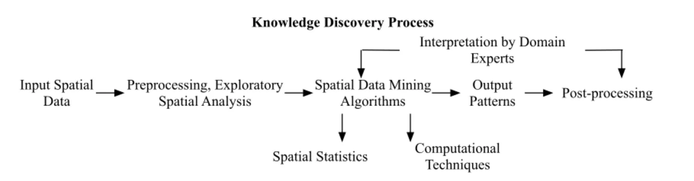
Spatial data mining studies the process of discovering interesting, previously unknown, but potentially useful patterns from large spatial databases [31, 32, 33, 34, 35, 12]. Fig-ure 1.1 shows the entire knowledge discovery process. The core components are spatial data mining algorithms which take input spatial data and produce desired output pat-tern families, including spatial outliers, spatial interactions, spatial predictive models,

(15)

spatial partitions and summarizations, and hotspots. These algorithms have statisti-cal foundations and integrate sstatisti-calable computational techniques which follow certain mathematical properties such as correctness and completeness.

Input Spatial Data

Preprocessing, Exploratory Spatial Analysis

Spatial Data Mining Algorithms

Output

Patterns Post-processing

Spatial Statistics Computational Techniques

Interpretation by Domain Experts

Knowledge Discovery Process

Figure 1.1: The process of spatial data mining

add: how is it different from traditional data mining (input data, auto-correlation, pattern families)

1.1.1 Societal Importance

Spatial data mining plays a critical role in many applications domains and across various governmental agencies. For example, NASA needs spatial data mining tools to classify earth observation images into land cover maps for ecology and environment manage-ment [36]. The National Institute of Health (NIH) uses spatial data mining tools to detect disease outbreaks for public health [37]. Law enforcement officers leverage spa-tial data mining techniques to help discover crime patterns [28]. The US Department of Transportation analyzes patterns (e.g., accident hotspots) in traffic data to improve transportation safety and efficiency [1]. Also, vehicle GPS trajectories together with en-gine measurements (e.g., fuel consumption, emission) are mined to recommend routes that are fast, fuel efficient, or environmental friendly [29, 30]. There are also other application domains such as earth science, climatology, precision agriculture, and the Internet of Things. The US Coast Guard is interested in mining trajectory patterns from Automatic Identification System (AIS) data [38] to help detect violations of mar-itime regulation such as illegal, unreported and unregulated (IUU) fishing and illicit

(16)

transactions [10].

The interdisciplinary nature of spatial data mining requires that its techniques be developed with an awareness of domain knowledge (e.g., underlying physics, theoretical assumptions) from the application disciplines [34, 39]. For example, climate science re-search finds that observable predictors for climate phenomena discovered by purely data driven methods can be misleading without consideration of climate models, locations, and seasons [40].

1.1.2 Spatial Statistical Foundations

Spatial statistics [41, 42, 43, 44] is a branch of statistics focusing on the analysis and modeling of spatial data. It is special due to the unique characteristics of space. For ex-ample, according to the first law of geography: “Everything is related to everything else, but near things are more related than distant things” [45]. Known as spatial autocorre-lation, such spatial dependency across nearby locations violates the common assumption in classical statistics that variables are independent and identically distributed.

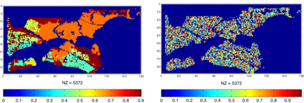
An illustration of the spatial autocorrelation phenomenon in the real world can be seen in Figure 1.2. Figure 1.2(a) shows a map of the distribution of vegetation durability across a marshland. The spatial autocorrelation effect can be seen from the fact that neighbor regions tend to have similar colors. By contrast, Figure 1.2(b) shows what the map would look like if vegetation durability followed an independent and identical distribution, which looks very different from the reality.

A spatial point process is a stochastic process for mining patterns from spatial point data. Unlike point reference data, the random variables are locations rather than non-spatial attributes. Examples include locations of crime events in a city. One basic type of spatial point process is a homogeneous spatial Poisson point process (also called complete spatial randomness, or CSR) [43], where point locations are independent following a homogeneous intensity over space. Figure 1.3 shows an example data set following CSR.

However, real world spatial point processes are often not completely spatial random. First, spatial aggregation (clustering) or spatial inhibition between point locations often exists as opposed to complete spatial independence as in CSR. Spatial statistics such as Ripley’s K function [46] (the average number of points within a certain distance

(17)

NZ = 5372

0 0.1 0.2 0.3 0.4 0.5 0.6 0.7 0.8 0.9

(a) Actual vegetation durability distribution with spatial autocorrelation

NZ = 5372

0 0.1 0.2 0.3 0.4 0.5 0.6 0.7 0.8 0.9 NZ = 5372

(b) Vegetation durability distribution with i.i.d. assumption

Figure 1.2: A real world example of spatial autocorrelation effect

0 20 40 60 80 100 0 10 20 30 40 50 60 70 80 90 100

SatScan output with a continuous Poisson model on a CSR dataset

!! "#$%&'()*+,-100 80 60 40 20 0 20 40 60 80 100

Figure 1.3: An example of complete spatial randomness

of a given point normalized by the overall intensity) can be used to test for spatial aggregation within a point pattern. Second, real world spatial point processes such as crime events often contain hotspot (significantly high intensity) areas instead of following homogeneous intensity across space. A spatial scan statistic [47] can be used to detect these hotspot patterns. The statistic uses a regular shaped window to scan the study area and test if point intensity within the window is significantly higher than outside. Though both the K-function and spatial scan statistics employ the same null hypothesis of CSR, their alternative hypotheses are quite different: The K-function tests whether points exhibit spatial aggregation or inhibition rather than independence, while spatial

(18)

scan statistics assume that points are independent and test whether a hotspot with much higher intensity exists. Finally, there are other spatial point processes such as the Cox process, in which the intensity function itself is a random function over space, as well as a cluster process, which extends a basic point process with a small cluster centered on each original point [43].

Besides spatial point process which deals with spatial point data, other spatial statis-tic models have been proposed for other types of data as well [41, 42, 43, 44].

Geostatistics [44] deals with the analysis of the properties of point reference data, including spatial continuity (i.e., dependence across locations), weak stationarity (i.e., first and second moments do not vary with respect to locations) and isotropy (i.e., uniformity in all directions). For example, under the assumption of weak stationarity (or more specifically intrinsic stationarity), the variance of the difference of non-spatial attribute values at two point locations is a function of point location difference only, regardless of the specific locations of the points. This function is called a variogram [41]. If the variogram only depends on distance between two locations (not varying with respect to direction), it is further called isotropic. Under the assumptions of these properties, geostatistics also provides a set of statistical tools such as Kriging [41], which can be used to interpolate non-spatial attribute values at unsampled locations. In addition, real world spatial data may not always satisfy the stationarity assumption. For example, different jurisdictions tend to produce different laws (e.g., speed limit differences between Minnesota and Wisconsin). This effect is called spatial heterogeneity or non-stationarity. Special extended models (e.g., geographically weighted regression, or GWR [48]) can be used to model the varying coefficients at different locations. For example, in traditional linear regression model: y =Xβ+, weight β and noise are location independent. However, in spatial linear regression, they are location dependent and vary over different locations.

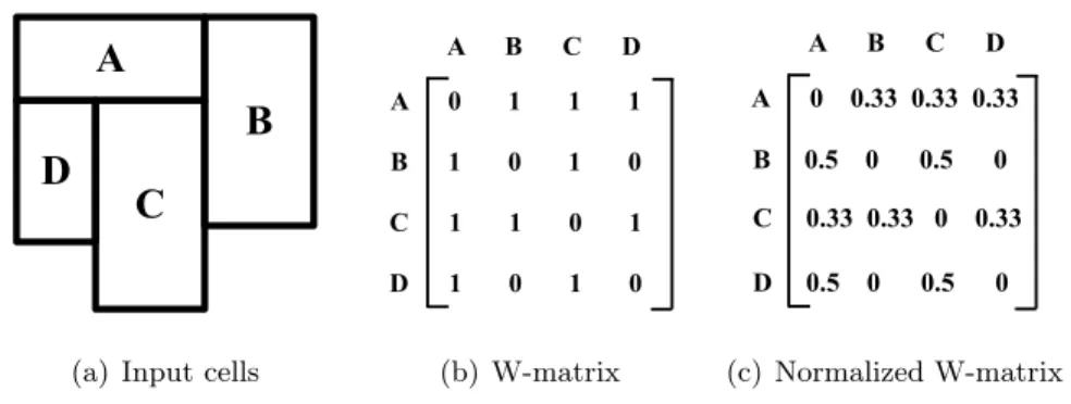
Lattice statistics analyzes and models non-spatial attributes in a lattice (areal) model. One key issue in lattice statistics is to model the dependency across nearby cells. The range of such dependency is often represented by a neighborhood (or contiguity) matrix called a W-matrix. W-matrix elements (spatial neighborhood relationships) can be defined based on spatial adjacency (e.g., rook or queen neighborhoods), Euclidean distance, or in more general models, cliques and hypergraphs [49]. Figure 1.4(a) shows

(19)

an example of four cells and Figure 1.4(b) gives the W-matrix of these cells. If two cells are neighbors, the corresponding element in the matrix is 1. Figure 1.4(c) gives a normalized W-matrix in which the total values in each row is 1 unless all elements are 0 in the row.

A

B

C

D

(a) Input cells

A B C D A 0 1 1 1 B 1 0 1 0 C 1 1 0 1 D 1 0 1 0 (b) W-matrix A B C D A 0 0.33 0.33 0.33 B 0.5 0 0.5 0 D 0.5 0 0.5 0 C 0.33 0.33 0 0.33 (c) Normalized W-matrix

Figure 1.4: An example of W-matrix

Based on a W-matrix, spatial autocorrelation statistics can be defined which reflect the correlation of non-spatial attribute values at neighboring locations. Common spatial autocorrelation statistics include Moran’s I, Getis-OrdGi∗, Geary’sC, Gamma index Γ [44], etc., as well as their local versions called local indicators of spatial association (LISA) [50]. A high spatial autocorrelation means non-spatial attribute values at nearby locations tend to be very similar. There are also several lattice statistics models, such as the spatial (or simultaneous) autoregressive model (SAR) and conditional autoregressive model (CAR), both of which belong to a more general family called Markov random fields (MRF). SAR directly models spatial dependency across response variables at different locations, while CAR models the dependency in conditional probability. A CAR model is often used as an additional term for capturing spatial autocorrelation in other Bayesian hierarchical models [41]. Another important issue in lattice statistics is the modifiable areal unit problem (MAUP) (also called the multi-scale effect) [51], which tells us that the same analysis method will show various results on different aggregation scales. For example, analysis using data aggregated by states will differ from analysis using data aggregated by counties.

(20)

1.1.3 Spatial Pattern Families

Spatial data mining outputs various patterns depending on the application needs and computational techniques. Now we go through some example pattern families that have been widely studied and applied, namely spatial outliers, co-locations, and spatial hotspots.

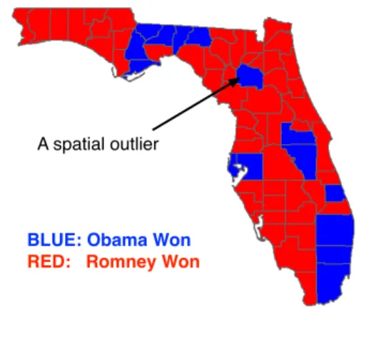
Spatial outliers: Global outliers are observations that appear to be inconsistent with remaining observations, or which deviate so much from other observations as to arouse suspicions that they were generated by a different mechanism. In contrast, a spa-tial outlier [52, 53] is a spaspa-tial object whose non-spaspa-tial attributes deviate significantly from those of its spatial neighbors. Informally, a spatial outlier is a local instabil-ity or discontinuity. For example, a new house in an old neighborhood of a growing metropolitan area is a spatial outlier but not a global outlier based on house age. In the county-level voting results of the 2012 U.S. presidential election in Florida shown in Figure 1.5, the lone county in the upper middle of the map voted for Obama while all its neighbors voted for Romney can be considered a spatial outlier.

BLUE: Obama Won

RED: Romney Won A spatial outlier

Figure 1.5: An illustrative example of a spatial outlier: voting results of 2012 U.S. president election in Florida

In transportation, spatial outlier indicates anomalous traffic patterns from sensor observations on a highway road network. In mobile banking, spatial outlier detection can help provide early warning for fraud transactions.

(21)

and neighborhood approaches. Visualization approaches identify spatial outliers via plotting of spatial locations on a graph. Common methods are variogram clouds [54] and Moran scatterplots [50, 44] as introduced earlier.

Neighborhood approaches begin by defining a spatial neighborhood, and then com-pute a test statistic (i.e., outlier score) based on the difference on non-spatial attributes between the current location and the neighborhood aggregate [52]. Spatial neighbor-hoods can be defined by geographical distances (e.g., K nearest neighbors), or by topo-logical connectivity (e.g., adjacent nodes on road networks). The fundamental spatial outlier detection methods have been extended in a number of directions. Typical ap-proaches focus on numerical attributes whose values are naturally ordered and thus able to be arithmetically operated (e.g., housing price). However, they are not able to han-dle categorical attributes such as housing colors. To solve the categorical spatial outlier problem, approaches based on measuring correlation between the occurrence pattern of categorical attribute values have been proposed [55, 56]. Spatial outlier detection with multiple non-spatial attributes [57, 58] finds a way to combines different non-spatial attributes to obtain the comprehensive outliers. Weighted spatial outlier detection [59] takes the impact of the neighbors of an object into consideration. Local variance-aware spatial outlier detection approach [60] considers the heterogeneity of variance, that is, the outlier score is computed based on not only the extent of variance but the average variance in that area.

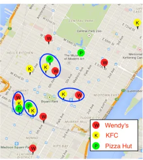
Co-locations: Co-location patterns [61], represent subsets of spatial event types whose instances are often located in close geographic proximity. Real-world examples include symbiotic species in ecology, e.g., the Nile Crocodile and Egyptian Plover and commercial localization, e.g., fast food restaurants tend to open near other fast foot restaurants. Figure 1.6 shows an example of locations of Wendy’s (“W”), KFC (“K”), and Pizza Hut (“P”) in Manhattan, New York City. Some patterns that stores are open close to each other are observed, namely “W-K-P”, “P-K”, and “W-K”.

Discovering various patterns of spatial co-location is important in applications re-lated to ecology, environmental science, public safety, and climate science. For example, identifying spatially co-located crime types can help police departments to understand crime generators in a city, and thus take effective measures to reduce crime events.

(22)

W W W W W W W P P P K K K K K K P P W K Wendy's KFC Pizza Hut

Figure 1.6: Illustration of Point Spatial Co-location Patterns. Different colors represent different spatial feature types. together

Different computational approaches have been developed to identify spatial co-locations. Traditional approaches use the cross-K function with Monte Carlo sim-ulation [44], mean nearest-neighbor distance, and the spatial regression model [62]. Other approaches use an event centric model [61] based on a defined monotonic interest measure, participation index, which is an upper bound of cross-K function statistics, allowing efficient algorithms via apriori-based upper-bound pruning. Within the same framework, another interest measure, called the probabilistic participation index [63] deals with the uncertainty of spatial features caused by over-counting of the data. Also, maximal participation ratio [64] has been proposed to find patterns that involve object types having mismatched frequency. In order to take spatial heterogeneity into account, researchers have developed regional spatial co-location detection approaches which find object types that are highly correlated in certain sub-regions [65, 66, 67]. To minimize the cost of false positives, approaches that use statistical significance test to eliminate chance patterns have also been proposed [65, 68].

Spatial hotspots: Spatial hotspot detection finds regions where the number of events is significantly high. Figure 1.7 shows a real world spatial hotspot example from

(23)

the 1854 London Cholera outbreak detected by a popular tool, SaTScan [47, 69].

(a) Input Cholera cases (b) Circular hotspot detected by SatScan

Figure 1.7: A real world example of spatial hotspot in 1854 London Cholera outbreak Spatial hotspot detection helps find disease outbreaks which allows officials to allo-cate resources to limit its spread [47, 69]. In criminology, finding crime hotspots may help police officials distribute their force on most critical regions and even help search for a criminal.

Spatial scan statistics [47, 69], the most popular spatial hotspot detection approach assumes that activities diffuse isotropically on Euclidean space and this it detects sta-tistically significant hotspots in a circular/elliptical shape. A number of newer ap-proaches [70, 71, 72, 73, 74] have been proposed which overcome the limitation of isotropic diffusion. More recent approaches deal with hotspots of events occurring on spatial networks [75, 76, 77]

Other approaches include Kernel density estimation (KDE) [78] which identifies hotspots via a density map of point events. First, a grid is created over the study area and a kernel function is used with a user-defined radius (bandwidth) on each point to estimate the density of points on centers of grid cells. A subset of grid cells with high density are returned as spatial hotspots. The Geographical Analysis Machine (GAM) method [79] first creates a regular grid in the study area, draws circles with a fixed radius around the grids, and identifies the ‘dense’ circles whose numbers of points are significantly higher than expected values. Finally, GAM merges overlapping dense circles and connected components as spatial hotspots.

(24)

1.2 Challenges

The challenges of spatial data mining come from three aspects: statistics, computing, and mathematics.

Spatial data mining poses unique statistical challenges due to the special character-istics of spatial data. First, spatial data are embedded in continuous space and time, and thus many classical data mining techniques assuming disjoint data (e.g., transac-tions in association rule mining) may not be effective. Second, spatial data exhibits spatial autocorrelation effects. Ignoring autocorrelation and assuming an identical and independent distribution (i.i.d.) when analyzing spatial data may produce hypotheses or models that are inaccurate (e.g., salt and pepper noise, pixels predicted as different from neighbors by mistake) [80]. Third, interactions are non-isotropic (varying across spatial directions) and may exist in multiple spatial scales. In addition to spatial depen-dence at nearby locations, phenomena of spatial tele-coupling also indicate long range spatial dependence such as El Nino and La Nina effects in the climate system. Finally, spatial data exhibits spatial heterogeneity and temporal non-stationarity, i.e., identical feature values may correspond to distinct class labels in different spatial regions.

The computational challenges are due to the huge amount of spatial data and the cost of identifying complex patterns. For example, on-board diagnostic data collected every day from millions of running vehicles can be in petabytes and contain hundreds of variables (e.g., speed, emission). Identifying the combinations of negatively corre-lated variables requires enumerating exponential of the number of variables, leading to intractable computational cost. In addition, statistical significance test needs to be en-forced in certain patterns due to the potentially unacceptable cost from false positives. For example, a falsely identified crime hotspot may cause panic and a drop in house prices in the neighborhood.

Spatial data mining algorithms need to ensure necessary mathematical properties of the output patterns such as correctness and completeness. Correctness indicates that the algorithm is able to terminate and the output patterns must all the solution requirements. For example, a hotspot must pass the statistical significance test (i.e., p-value ≤threshold) to be considered an output. Completeness indicates that no patter that meets all the solution requirements is missed in the output. For example, the

(25)

spatial scan statistics [47, 69] detects circular hotspots defined by two events, one at the center and the other on the circumference. To ensure completeness, it needs to enumerate all such circles defined by two points. Completeness is always associated with a specific pattern definition which typically involves a trade-off between computational tractability and richness of the pattern. For example, even though the spatial scan statistics [47, 69] achieves completeness for circular hotspots defined by two points, it is not able find any hotspots whose center has no event. Worse, it misses all the hotspots that are not circular.

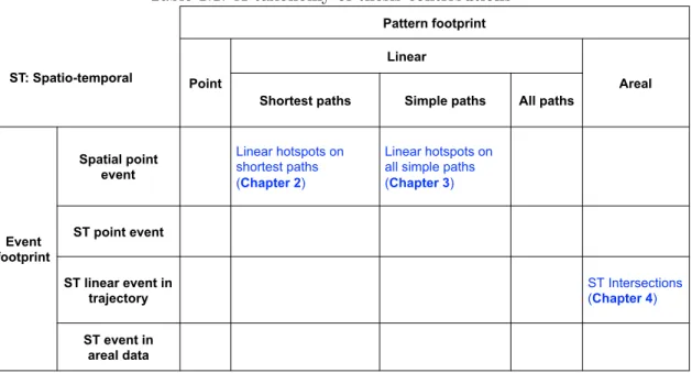
1.3 Thesis Contributions

This thesis investigates data science techniques for mining patterns from various foot-prints of spatial events. The contributions are summarized in a taxonomy shown in Table 1.1 which describes the input spatial events and output spatial patterns classified by their footprints. The input spatial events are classified into four types: First, a spatial point event is modeled as a static 2-D point (x, y) representing the location where the event occurs and the temporal information is omitted. For example, all traffic accidents occurring on a street over a year can be modeled as a collection of spatial point events. One step beyond the spatial point event is the a spatio-temporal point, which takes tem-poral information into account and can be modeled as a 3-D point (x, y, t) representing an event located at (x, y) at time t. For example, when studying the pattern of traffic accidents on a street at different times of day, a traffic accident can be modeled as a spatio-temporal point event. The third event footprint studied is the spatio-temporal linear event, which is represented a sequence ofN 3-D points (xi, yi, ti), i= 1...N which

are typically extracted from trajectories. For example, the trajectory of a vehicle speed-ing durspeed-ing a period of time can be modeled as a spatio-temporal linear event. Lastly, we examined the spatio-temporal event in areal data, which occurs on a sequence of matrices of pixels where each pixel represents attributes in the corresponding space and time. One example is a spreading forest fire that appears on remote sensing imagery. As with the input events, the output spatial patterns are classified as point, linear, or areal patterns. Based on the different complexities of the enumeration space, linear patterns can be further classified into shortest paths, simple paths, or all paths.

(26)

This thesis proposes several novel spatial data mining approaches (i.e. linear hotspot discovery on shortest paths, linear hotspot discovery on all simple paths, and spatio-temporal intersection detection from trajectories with data gaps) which address the statistical, computational, and mathematical challenges posed by various footprints of input spatial events and output patterns. Not only do the proposed approaches achieve high computational efficiency but also the statistical and mathematical properties are well studied. The content of each chapter is briefly introduced below.

Table 1.1: A taxonomy of thesis contributions

Pattern footprint

Point

Linear

Areal

Shortest paths Simple paths All paths

Event footprint Spatial point event Linear hotspots on shortest paths (Chapter 2) Linear hotspots on all simple paths (Chapter 3) ST point event ST linear event in trajectory ST Intersections (Chapter 4) ST event in areal data ST: Spatio-temporal

• Chapter 2 presents a novel hotspot detection approach, Linear Hotspot Discovery on Shortest Paths (LHDSP), which finds all shortest paths on a spatial network where the concentration of input spatial point events is statistically significantly high. The method addresses the limitation of traditional spatial hotspot detec-tion approaches only focusing on hotspots in Euclidean space. LHDSP has many societal application fields such as transportation planning where the events (e.g., traffic accidents) are usually associated with linearly shaped roadways. LHDSP proposes multiple novel algorithms, namely neighbor node filter and shortest path

(27)

tree pruning, to successfully handle the computational challenges from large num-ber of candidate paths, non-monotonicity of the test statistic, and statistical sig-nificant test. To balance between computational tractability and richness of the pattern, LHDSP assumes that most travelers prefer to move along shortest paths. Under this assumption, LHDSP enumerates all shortest paths on a given spatial network and guarantees correctness and completeness of the solution. Theoretical and experimental analyses show that the proposed algorithms yield substantial computational savings compared to baseline approaches. Case studies demon-strate that LHDSP can find novel linear patterns that have never been detected previously.

• Chapter 3 investigates the problem of Linear Hotspot Discovery on All Simple Paths (LHDA) which considers much richer patterns compared to LHDSP (pro-posed in Chapter 2) does by enumerating all simple paths on a given spatial network. To address this much more difficult computational challenge (i.e. #-p hard), LHDA proposes a novel algorithm based on bi-directional fragment-multi-graph traversal (i.e. ASP FMGT). Extensive theoretical and experimental analy-ses show that ASP FMGT has substantially improved performance over a baseline approach using depth-first-search with backtracking while keeping the solution correct and complete. Case studies on real-world datasets show that ASP FMGT outperforms existing approaches including LHDSP since it discovers new hotspots unknown before and achieves higher accuracy for locating known hotspots.

• Chapter 4 investigates the problem of Spatio-temporal Intersection Detection From Trajectories With Data Gaps (STID) which aims to identify meet-up pat-terns between objects (e.g., ships, vehicles) whose trajectories have missing seg-ments (i.e. Spatio-temporal Intersection (STI) pattern) from large scale spatio-temporal linear events. The applications of STID include maritime safety and regulation, homeland security, and public safety. STID overcomes the limitation of traditional trajectory mining approaches which assume the availability of tra-jectory data or interpolate the missing segments. It also addresses the computa-tional challenge from the huge amount of trajectory data and the high complexity of the STI pattern with an apriori-graph traversal based algorithm AGT STID.

(28)

Both theoretical and experimental analyses show that AGT STID significantly increases the computational performance over baseline approaches and guaran-tees solution correctness and completeness. A case study on real-world maritime trajectory data demonstrates AGT STID is able to discover previously unknown meet-up patterns and thus reveal possible illicit maritime transaction activities.

• Chapter 5 summarizes the thesis findings and gives an overview of related direc-tions and topics for research in the future.

(29)

Chapter 2

Linear Hotspot Discovery on

Shortest Paths

2.1 Introduction

Linear Hotspot Discovery on Shortest Paths (LHDSP) identifies routes with statisti-cally significant concentrations of activities (e.g., crimes, accidents, etc.). Informally, the LHDSP problem can be defined as follows: given a spatial network, a collection of geo-referenced activities (e.g., pedestrian fatality reports, crime reports), and a con-centration of activities threshold θd, find all shortest paths between activities in the

spatial network where the concentration of activities is unusually high (i.e., statistically significant) and the concentration of activities is equal to or greater thanθd. Depending

on the domain, an activity may be the location of a pedestrian fatality, a carjacking, a train accident, etc. Figure 2.1 illustrates an input example of LHDSP consisting of 7 nodes, 7 edges (with edge weights set to 1 for illustration purposes), 10 activities (shown as squares on the edges), and θd= 12, indicating that we are interested in the shortest

paths between activities whose concentrations of activities is equal to or greater than

θd= 12.

(30)

N N N5 N4 A1 A2 A3 A4 A5 A6 A7 A8 A9 3 6 N7 N5 N N4 N1 2 2 1.75 1.5 1.25 1 0.75 0.5 0.25 0 0 0.25 0.5 0.75 1 1.25 1.5 1.75 2 A10

Figure 2.1: Example of input of Significant Linear Hotspot Discovery (Best in color).

2.1.1 An Illustrative Application Domain: Preventing Pedestrian Fa-talities

Urban computing aims to handle the major issues that cities face by using computa-tional techniques. Seven major urban computing categories are urban planning, trans-portation, environment, energy, social, economy, and public safety and security [81]. Our proposed work focuses on discovering the statistically significant linear hotspots on road networks to address the issues associated with two of these application domains namely transportation planning and public safety and security.

To illustrate the applicability of Linear Hotspot Discovery on Shortest Paths (LHDSP), we focus on the problem of discovering significant concentrations of pedestrian fatali-ties in a transportation network. According to a recent policy report, more than 47,700 pedestrians were killed in the United States from 2000 to 2009 [1], and more than 688,000 pedestrians were injured over the same time period, which is equivalent to a pedestrian being struck by a vehicle every 7 minutes. Pedestrian fatalities have increased in many places, including 15 of the country’s largest metro areas, even as overall traffic deaths have fallen [1].

Domain experts attribute pedestrian fatalities largely to the design of streets, which have been engineered for speeding traffic with little or no provision for people on foot, in wheelchairs or on bicycles [1]. Daily activities have shifted away from city streets towards

(31)

(a) (b) (c)

Figure 2.2: (a) Pedestrian at risk on a road without proper sidewalks [1]. (b) Paved side-walk and road separators for pedestrians, bicycles, and motorcycles build on road [2]. (c) Pedestrian fatalities occurring on arterials in Orange County, FL [3] (Best in color).

higher speed arterials. This has resulted in more than half of fatal pedestrian crashes occurring on these wide, high capacity and high-speed thoroughfares. Typically designed with four or more lanes and high travel speeds, arterials are not built with pedestrians in mind (Figure 2.2(a)). They lack sidewalks, crosswalks (or have crosswalks spaced too far apart), pedestrian refuges, street lighting, and school and public bus shelters [1].

This lack of basic infrastructure can be lethal. For example, forty percent of fatalities occurred where no crosswalk was available [1]. Figure 2.2(c) shows a map of pedestrian fatalities that occurred on Orange County roads from 2000 to 2009. Transportation planners and engineers need tools to assist them in identifying which frequently used road segments/stretches pose statistically significant levels of risk for pedestrians and consequently should be redesigned. A promising way to effectively discover such road segments/stretches raises from the availability of the large amount of fatality data and corresponding data analysis approaches [81]. Road segments/stretches that pose sig-nificant risks to pedestrians may be conceptualized as linear concentrations because the generation model of pedestrian fatalities is inherently linear, i.e., they occur on roads. This chapter presents an approach for identifying statistically significant linear concentrations of activities such as pedestrian fatalities in a spatial network.

If traditional hotspot discovery is used (e.g., circular hotspot detection), the gov-ernment can just fix the hotspots for the pedestrian. However, often such hotspots do not occur on a circular area and the fix of those hotspot locations requires a road to be analyzed for structural mistakes by the transportation planners. The Minnesota

(32)

Department of Transportation proposes that building lane separators for pedestrian sidewalks, bicycles and motorcycles along roads illustrated in Figure 2.2(b) as a way to decrease the risk of traffic accidents [2]. In addition, lack of barriers between opposite traffic on specific parts of highways may lead to severe traffic accidents. For example, since Spring 2015, there were two fatal traffic accidents occurred on Minnesota Highway 280 at similar locations. The cars that lost control went to the flowing traffic on the opposite side since no barriers were in between along the highway segment [82].

Traditional network-based techniques which consider edges atomic face a funda-mental limitation in dealing with very long edge with a dense cluster of activities at one end of the edge. These techniques may either fail to capture the precise locations of the hotspots on such edges or even completely miss the hotspots. For example in Figure 2.1, hN1, N2i is an edge whose activities are densely clustered near N2 (i.e.,

A1, A2, A3, A4). Traditional techniques may capture hN1, N2i as a hotspot, however,

the precise location which is actually hA1, A4i is not captured. In worse case, suppose

the concentration of hA1, A4i exceeds the threshold but the overall concentration of

the entire path hN1, N2i does not since it is compromised by the empty end hN1, A1i,

this hotspot will be completely missed. To address this limitation, domain experts in-troduces dynamic segmentation which segments edges into sub-edges at each activity. This chapter investigates dynamic segmentation in order to evaluate if paths between activities are hotspots. For example, hA1, A4iwill be returned as a hotspot with a more

precise location thanhN1, N2ireturned by the traditional techniques. In the other case

that hN1, N2i is not qualified as a hotspot, hA1, A4i may also be return as a hotspot.

The technical details ofdynamic segmentation are elaborated in the problem statement (Section 2.2). The significance of using dynamic segmentation is demonstrated in the case studies on real datasets (Section 5).

Linear hotspot discovery can also be applied to other application domains. Certain types of crimes (e.g., assaults, street robbery) may form hotspots on transportation networks that represent roads needing more attention from police departments [3]. In addition, water quality changes on river networks may form hotspots that represent bursts of pollution [83].

(33)

2.1.2 Challenges

LHDSP is challenging due to the potentially large number of candidate routes (∼1016) in a given dataset with millions of activities and road segments. Enumerating and evaluating all shortest paths at the sub-edge level results in prohibitive computational cost. Additionally, density ratio does not obey the monotonicity property, meaning that there is no ordering between the density ratio of a path and its super-paths, or vice-versa. Furthermore, depending on the method used to determine statistical significance, computation times may also be impacted (e.g., m= 1000 Monte Carlo simulations may be required to calculate statistical significance).

2.1.3 Related Work and Their Limitations

Dividing spatial data into statistically significant groups is an important task in many domains (e.g., transportation planning, public health, epidemiology, climate science, etc.). Methods for this type of partitioning may generally be considered to be geometry-based or network-geometry-based.

Geometry-based techniques [84, 4] partition spatial data using geometric shapes (e.g., circles, rectangles). This is useful in domains such as public health, where finding spatial clusters with a higher density of disease is of interest for understanding the distribution and spread of diseases, outbreak detection, etc. Kulldorff, et al. proposed a spatial scan statistics framework (and the SaTScan software) for disease outbreak detection [47]. The spatial scan statistic employs a likelihood ratio test where the null hypothesis is the probability that disease occurrence inside a region is the same as outside, and the alternative hypothesis is that there is a higher probability of disease inside than outside. All the spatial regions, represented by a circle or ellipsoid in the spatial framework, are enumerated and the one that maximizes the likelihood ratio is identified as a candidate. However, if we apply SaTScan to a road network, many significant routes may be missed since a large fraction of the area bounded by circles for activities on a path will be empty. Figure 2.3(a) shows an example of the output of SatScan. Two circular hotspots are detected with large empty areas, which result in high p-values (i.e., 0.125 and 0.497). Furthermore, geometry-based techniques may not be appropriate for modeling linear clusters, which are formed when the underlying

(34)

generator of the phenomena is inherently linear (e.g., pedestrian fatalities, railroad accidents, etc.). N N N5 N4 A1 A2 A3 A4 A5 A6 A7 A8 A9 3 6 N7 N5 N N4 N1 2 2 1.75 1.5 1.25 1 0.75 0.5 0.25 0 0 0.25 0.5 0.75 1 1.25 1.5 1.75 2 A10 p-value = 0.125 p-value = 0.497 (a) N N N5 N4 A1 A2 A3 A4 A5 A6 A7 A8 A9 3 6 N7 N5 N N4 N1 2 2 1.75 1.5 1.25 1 0.75 0.5 0.25 0 0 0.25 0.5 0.75 1 1.25 1.5 1.75 2 A10 (b) N N N5 N4 A1 A2 A3 A4 A5 A6 A7 A8 A9 3 6 N7 N5 N N4 N1 2 2 1.75 1.5 1.25 1 0.75 0.5 0.25 0 0 0.25 0.5 0.75 1 1.25 1.5 1.75 2 A10 Root (c)

Figure 2.3: Example (a) Output of SatScan [4], (b) Output of Linear Intersecting Paths (LIP) [5], and (c) Output of Constrained Minimum Spanning Trees (CMST) [6] (Best in color).

By contrast, network-based techniques [6, 5, 85] leverage the underlying spatial network when partitioning spatial data. For example, Linear Intersecting Paths (LIP) [5] and Constrained Minimum Spanning Tree (CMST) [6] utilize a subgraph (e.g., a path or tree) to discover statistically significant groups.

LIP [5] discovers one anomalous sub-component of a set of connected paths that intersect each other. The connected paths are based on locations in the spatial network

(35)

with the highest percentage of activities, specified by the user. Hence the density ratio is evaluated only on a portion of the graph specified by this percentage, not on the entire spatial network. Figure 2.3(b)(b) shows an example of the output of LIP. The user-specified percentage is 40%, which means all the candidates will have paths containing edgehN1, N2isince this edge has 4 activities (out of 10 activities). Examples of possible

candidates arehN1, N3i,hN1, N5i,hN2, N4i,hN1, N7i, etc. The output ishN1, N3i, since

it has the highest density ratio. However, in addition to returning only one statistically significant component, the results of this approach are sensitive to the percentage of the network selected. If the percentage is too high, the number of candidates may be highly restricted, which could result in not identifying statistically significant regions of interest. If the percentage is too low, LIP may be computationally prohibitive due to the large number of candidates.

Another network-based technique, CMST [6], finds one statistically significant tree in the spatial network. Figure 2.3(c) shows an example of the output of CMST. Here the output is hN1, N3i, where N2 is the root, since this tree has the highest density

ratio. However, this approach also has limitations. In addition to returning only one statistically significant tree, the size of the tree is restricted, which could result in not identifying statistically significant regions of interest.

2.1.4 Contributions

In this chapter, we present a new dynamic segmentation model which to the best of our knowledge is the first model that allows for discovering of multiple statistically significant routes at the sub-edge level in a spatial network. We present new algorithmic refinements (i.e., neighbor node filter, shortest path tree pruning) for sub-edge level linear hotspot discovery in a scalable way. We also present a cost model for the proposed algorithms and prove that our proposed algorithmic refinements are correct. Specifically, our research contributions are as follows:

• We propose a new model named dynamic segmentation, which allows the proposed approach to find multiple significant linear hotspots at the sub-edge level in the spatial network. We also introduce new algorithmic refinements to improve the scalability of linear hotspot detection with dynamic segmentation, including a

(36)

neighbor node filter and a shortest path tree pruning algorithm.

• We analytically prove the correctness of the proposed algorithms and present a cost analysis.

• We present two case studies comparing the detection results under dynamic seg-mentation with results in the related works, including SRM GIS [86] and SatScan [4].

• Experimental results on real and synthetic data show that the proposed algo-rithms, yield substantial computational savings over SRM GIS [86] without re-ducing either completeness or correctness of the result.

2.1.5 Scope and Outline of the Chapter

This chapter focuses on finding significant discrete activity events (e.g., pedestrian fatal-ities, crime incidents) associated with a point on a network. This does not imply that all activities must necessarily be associated with a point in a street. In addition, other net-work properties such as GPS trajectories and traffic densities of road netnet-works [87, 88] are not considered. In this work, it is assumed that the number of activities on the road network is fixed and does not change over time. We do not consider techniques that do not employ statistical significance (e.g., DBScan [89], K-Means [90], KMR [91], and Maximum Subgraph Finding [92]). This chapter only enumerates shortest paths rather than all possible paths. This increases the computational tractability since the enumeration space decreases from exponential to polynomial. We choose shortest paths based on the assumption people generally prefer taking shortest paths a destination. Discovering hotspots on shortest paths may find the most possible ”dangerous” routes between two locations.

The chapter is organized as follows: Section 2.2 presents the basic concepts and prob-lem statement of Linear Hotspot Discovery on Shortest Paths (LHDSP). Section 2.3 presents our preliminary results towards addressing LHDSP. Section 2.4 details our proposed approaches for discovering sub-edge level linear hotspots in a scalable way. Section 2.5 presents two case studies comparing the proposed significant network-based outputs (i.e., shortest paths) to a significant geometry-based output (e.g., circles) on pedestrian fatality data. The experimental evaluation is covered in Section 2.6. Sec-tion 2.7 presents a discussion. SecSec-tion 2.8 concludes the chapter and previews future

(37)

work.

2.2 Basic Concepts and Problem Statement

This section reviews several key concepts in LHDSP and presents a formal problem statement.

2.2.1 Basic Concepts

The basic concepts are defined as follows:

Definition 1 A spatial network G= (N, E) consists of a node set N and an edge set E, where each element n in N is associated with a pair of real numbers (x, y) representing the spatial location of the node in Euclidean space [93]. Edge set E is a subset of the cross productN×N. Each elemente= (ni, nj) in E is an edge that joins

node ni to node nj.

Figure 2.1 shows an example of a spatial network where circles represent nodes and lines represent edges. A road network is an example of a spatial network where nodes represent street intersections and edges represent streets.

Definition 2 An activity setA is a collection of activities. Anactivitya∈A is an object of interest associated with only one edge e∈ E and has a location in Euclidean space.

In transportation planning, an activity may be the location of a pedestrian fatality; in crime analysis, an activity may be the location of a theft. Some of the edges in Figure 2.1 are associated with a number of activities (e.g., edge hN1, N2i has 4 activities).

Definition 3 The activity coverage inside a path, ap, is the number of activities

on p. The activity coverage outside p is |A| −ap, where |A| is the total number of

activities in the spatial network, G.

For example, in Figure 2.1, the activity coverage inside pathhA9, N5, A8, N2, A5, A6iis

(38)

Definition 4 The weight inside a path,wp, is the sum of weights of all edges in p.

The weight outside p is |W| −wp, where |W|is sum of weights of all edges in G. In

transportation planning, weight may represent distance or travel time of the path. In Figure 2.1, the weight inside hA9, N5, A8, N2, A5, A6i is 1.75 whereas the weight

out-side this path is 7−1.75 = 5.25.

Definition 5 Thedensity ratio of path p, λp= ap

÷wp

(|A|−ap)÷(|W|−wp) [85, 47].

The density ratio of path p,λp is the ratio of the activity density inside pathp, _wap_p to

the activity densityoutside p, |A|−ap

|W|−wp. Table 2.1 lists 3 shortest paths from Figure 2.1,

namely hA9, A6i,hA4, A10i, and hA1, A7i. PathhA9, A6i contains activitiesA9,A8,A5

and A6 and has a weight of 1.75, hence its density is ₁_.4₇₅ while the density outside is 10−4

7−1.75. Therefore, the density ratio of path hA9, A6i is

4÷1.75

(10−4)÷(7−1.75) = 2. By similar

calculation, path hA4, A10i has a density ratio of 1.42 and path hA1, A7i has a density

ratio of 14.

The reason why we use density ratio as the test statistic in this chapter is two-fold. First, density ratio is in a family of metrics inspired from the hypothesis test in which the null hypothesis is ”the density inside and outside a path are equal” while the alternative hypothesis is ”the density inside a path is larger than outside”. These metrics are largely used in hotspot detection literature [47, 84, 94] and follow three properties [84]: (1) Given a fixed weight, the metric increases monotonically with activity coverage. (2) Given a fixed activity coverage, the metric decreases monotonically with weight. (3) Given a fixed ratio of activity coverage to the weight, the metric increases monotonically with the weight. Any metrics that follow these properties (e.g., log likelihood ratio [47]) can be directly applied in the proposed approaches without any algorithmic changes. Second, among these metrics, density ratio is widely used in the literature that deals with activities associated with spatial networks [85]. We use density ratio to make it easier to compare the proposed algorithms with the literature.

(39)

Table 2.1: Examples of density ratio.

Definition 6 An active edge is an edge e ∈ E that has 1 or more activities. An

active node is a node u joined by an active edge. An inactive node is a node that is

not joined by any active edges.

Definition 7 AnActive nodeis a node n∈N that at least one of its incident edges has 1 or more activities.

Edges hN1, N2i and hN2, N3i in Figure 2.1 are active edges because they each have

at least one activity, and nodesN1,N2,N3,N5,N6, andN7 are all active nodes because

they are all joined by active edges. By contrast, Node N4 is an inactive node because

it is not joined by any active edges.

Definition 8 A super-path of path p is any path sp that contains p, where sp is a subset of G. A sub-pathis a path making up part of the super-path.

For example, in Figure 2.1, hN1, N2, N5, N6i and hN1, N2, N5, N7i are super-paths of

hN1, N2, N5i. Conversely, hN1, N2, N5i is a sub-path ofhN1, N2, N5, N6i.

2.2.2 Problem Statement

The problem of Linear Hotspot Discovery on Shortest Paths (LHDSP) can be expressed as follows:

Given:

1. A spatial network G = (N, E) with a set of geo-referenced activities A, each if which is associated with an edge.

(40)

3. Ap-value threshold,θpand the corresponding number of Monte Carlo simulations

needed,m,

Find: All shortest pathsr ∈R withλr≥θλ,p-value≤θp

Objective: Computational efficiency

Constraints:

1. ri∈R is not a sub-path ofrj ∈R for∀ri, rj ∈R whereri 6=rj,

2. ∀ri∈R is not shorter than a minimum distance (φ) threshold θφ

3. Correctness and completeness

The spatial network input for LHDSP is defined in Definition 1. The θλ input is a

threshold indicating the minimum desired density ratio. Theθpinput is the desired level

of statistical significance andmis the corresponding number of Monte Carlo simulations needed for determining statistical significance. The output for LHDSP is all shortest paths between activities meeting the desired likelihood ratio and level of statistical significance. The shortest paths returned are constrained so that they are not sub-paths of any other path in the output. This constraint aims to improve solution quality by reducing redundancy in the paths returned. In addition, the distance of significant paths cannot be shorter than θφ. This constraint aims to avoid meaningless tiny paths

that have high density ratio (e.g., a path between two activities very close to each other may have a high density ratio).

Dynamic Segmentation: Our approach resolves statistically significant routes to the sub-edge level (i.e., routes between activities), which is not investigated in our previous work [86]. This requires a model called dynamic segmentation. Intuitively, it modifies the traditional network structure such that new nodes are formed at the locations of activities and new edges are added to connect these nodes.

The pseudocode in Algorithm 1 shows the process of dynamic segmentation. All the edges with a activities (where a > 0) are split into a nodes and a+ 1 edges (line 2). For clarification, in this model, the nodes before segmentation are referred to as static nodes, while the newly formed nodes, which are essentially activities, are referred to as dynamic nodes. The weights of the newly formed edges in the dynamically segmented network are then updated based on the distance between activities (line 3). In other

(41)

words, the weight of the dynamic edge formed between activity x and activity y will be updated to the distance between these two activities. Dynamic nodes are stored in

dynamicN odes, and newly formed edges are stored indynamicEdges(line 4).

For example, in Figure 2.1, activitiesA1,A2,A3, etc. become nodes in the spatial

network, and edgehN1, N2 is cut into several edges, namelyhN1, A1i,hA1, A2i,hA2, A3i,

hA3, A4i, and hA4, N2i.

The dynamic segmentation model enables us to evaluate paths that start and end with activities and may be in the middle of an edge. As such, the density ratios tend to be more precise since the extra portions of the path before the first activity and after the last activity are trimmed. Therefore, segments which were previously not tested for statistical significance or which may have been previously deemed “not significant” because they were on a long empty edge, may end up as part of the result. For example, in Figure 2.1, hA1, A2, A3, A4, N2, A5, A6, A7i and hN1, N2, N3i have the same set of

activities but the weight of hA1, A2, A3, A4, N2, A5, A6, A7i is less. In this case, the

density ratio for hA1, A2, A3, A4, N2, A5, A6, A7i is much higher (14 vs. 5.83), and the

p-value is smaller (0.001 vs. 0.006).

Algorithm 1 Dynamic Segmentation

Input:

1) A spatial network G= (N, E) with a set of geo-referenced activities with point locations on network nodes or edges and weight function w(u, v)>0 for each edge

e= (u, v)∈E (e.g., network distance)

Output: A dynamically segmented spatial networkGs derived fromG

Algorithm:

1: for each edges e∈G witha >0 activities do

2: Spliteintoanodes, na, and a+ 1 edges,ea

3: update weights of ea based on coordinates of activities

4: dynamicN odes←na,dynamicEdges←ea

Finding Significant Paths

Each shortest path in the spatial network is evaluated for statistical significance using Monte Carlo simulations to determine whether or not it is statistically anomalous. Here the null hypothesis states that the paths identified by the path density ratio are random or by chance alone. The density ratio is associated with a p-value to decide whether the null hypothesis should be rejected in the hypothesis test. The p-value is the probability

(42)

of obtaining a density ratio that is equal to or greater than than that observed by chance alone.

In the Monte Carlo simulations, each activity in the original graphG is randomly put on a location inGso that the number of activities on each edge is shuffled, forming a new graph Gs. Note that all the activities inGare present in Gs, with no activities

added or removed. We then compare the highest density ratio λmaxGs of randomized Gs with the density ratio of each path pi whose density ratio is equal to or greater

than the threshold in the original G. In a na¨ıve way, in order to compute λmaxGs

of Gs, all-pairs shortest paths in Gs need to be computed using Dijkstra’s algorithm

since shuffled activities are considered as nodes, making Gs a new graph. Then the

density ratios of these paths are evaluated. However, an algorithmic refinement named neighbor node filter (Section 4.1.1) is proposed to evaluate the density ratios without running Dijkstra’s algorithm on the whole graph. If the original value is smaller, then

c=c+ 1 for pathpi. The above process repeatsm, making the subsequent p-value c+1_m

for path pi. Paths whose p-values are less than or equal to the given p-value threshold

are deemed statistically significant.

2.3 Preliminary Results

We initially solved the LHDSP problem with a previously proposed algorithm (SRM GIS) [86] featuring two algorithmic refinements: Density Ratio Pruning and Monte Carlo Speedup. Note that even though SRM GIS was proposed to solve LHDSP without dynamic seg-mentation, it can also be directly applied to dynamically segmented networks. Before describing SRM GIS, we first review a na¨ıve algorithm (SRM Na¨ıve) that solves the LHDSP problem.

2.3.1 Na¨ıve Significant Route Miner (SRM Na¨ıve)

Algorithm 2 presents the pseudocode for the SRM Na¨ıve approach. The basic idea behind the algorithm is to find all statistically significant shortest paths in the dynami-cally segmented spatial network whose density ratio exceeds the thresholdθλ, under the

constraint that the shortest paths returned are not sub-paths of any other path in the output. Algorithm 2 proceeds by calculating all-pairs shortest paths, P, in the spatial

(43)

network (Line 2). Line 3 evaluates each shortest path inP to determine if it meets the given θλ to form aCandidatesset. In line 4, the statistical significance of each shortest

path in Candidates is evaluated and the significant routes are stored in SigRoutes. In order to assess statistical significance, all shortest paths in each of the m simulated graphs are used to calculate the p-value. In line 5, all paths inSigRoutes that are not sub-paths of any other path in SigRoutesare returned, and the algorithm terminates. The purpose of returning significant routes that are not sub-paths of any other path is to improve solution quality. For example, if hN1, N2i and hN1, N2, N3i are both found

to be significant, only hN1, N2, N3iis returned.

Algorithm 2 Na¨ıve Significant Route Miner (SRM Na¨ıve) Algorithm

Input:

1) A spatial network G= (N, E) with a set of geo-referenced activities with point locations on network nodes or edges and weight function w(u, v)>0 for each edge

e= (u, v)∈E (e.g., network distance), 2) A density ratio (λ) threshold, θλ,

3) A p-value threshold,θp,

4)m, indicating the number of Monte Carlo simulations, 5) A minimum distance (φ) threshold θφ

Output:

All routesr ∈R withλr≥θλ,φr ≥θφ and p-value significance level

Algorithm:

1: GDS ←dynamically segmentG

2: {Step 1:} P ←calculate all-pairs shortest paths in GDS

3: {Step 2:} Candidates←paths in P having λ≥θλ and φ≥θφ

4: {Step 3:} SigRoutes ← significant paths in Candidates using m Monte Carlo simulations

5: {Step 4:} return paths that are not sub-paths of any other path in SigRoutes SRM Na¨ıve Example: Figure 2.4 shows an example execution trace of SRM Na¨ıve. The spatial network has 7 nodes, 7 edges, and 10 activities with specific locations on the edges. The density ratio threshold θλ is set to 12, the p-value threshold θp is set to

0.001, and the minimum distance threshold θφ is set to 0.75.

In step 1, all-pairs shortest paths in the given dynamically segmented spatial network are calculated (only paths with high density ratios are shown in the figure). For example, the shortest path between nodes A1 and A2 is hA1, A2i. In step 2, the density ratio,

(44)

Input

Density ratio threshold = 12 p-value threshold = 0.01 Minimum distance threshold = 0.75

Step 1 Step 2 Step 3

Output N N N5 N4 A1 A2 A3 A4 A5 A6 A7 A8 A9 3 6 N7 N5 N N4 N1 2 2 1.75 1.5 1.25 1 0.75 0.5 0.25 0 0 0.25 0.5 0.75 1 1.25 1.5 1.75 2 A10

Figure 2.4: Example execution trace of Na¨ıve Significant Route Miner (SRM Na¨ıve). Circles represent nodes and lines represent edges.

φ ≥θφ are stored as candidates. In the figure, from the 6 paths listed whoseλ ≥θλ,

only the first two paths are considered as candidates since their distances meet or exceed the threshold. In step 3, the statistical significance of each candidate is calculated using Monte Carlo simulations (discussed next). Both of the 2 candidates meet the p-value threshold of 0.01. In step 4 (shown as the output), all paths among the significant paths that are not sub-paths of any other path are returned as significant routes. In this example, pathhA1, A2, A3, A4, N2, A5, A6, A7iare returned since it is the super-path

of the other candidate. To reduce the prohibitive computational cost of SRM Na¨ıve, a new algorithm (SRM GIS) is proposed in our previous work [86].

2.3.2 Significant Route Miner with Density Ratio Pruning and Monte Carlo Speedup (SRM GIS)

The SRM GIS algorithm uses filter and refine techniques (e.g., density ratio pruning and Monte Carlo speedup) to achieve computational savings. The filter and refine techniques may not change worst case complexity but they can reduce runtime in many cases. Density ratio pruning creates a boundary via an upper-bound density ratio such that not all destinations are visited from each source node. Some of the destinations