City, University of London Institutional Repository
Citation
:
Zhu, R. ORCID: 0000-0002-9944-0369, Dong, M. and Xue, J-H. (2018). Learning distance to subspace for the nearest subspace methods in high-dimensional data classification. Information Sciences, 481, pp. 69-80. doi: 10.1016/j.ins.2018.12.061This is the accepted version of the paper.
This version of the publication may differ from the final published
version.
Permanent repository link:
https://openaccess.city.ac.uk/id/eprint/21194/Link to published version
:
http://dx.doi.org/10.1016/j.ins.2018.12.061Copyright and reuse:
City Research Online aims to make research
outputs of City, University of London available to a wider audience.
Copyright and Moral Rights remain with the author(s) and/or copyright
holders. URLs from City Research Online may be freely distributed and
linked to.
City Research Online: http://openaccess.city.ac.uk/ [email protected]
Learning distance to subspace for nearest subspace
methods in high-dimensional data classification
Rui Zhua,b,c,∗, Mingzhi Dongc, Jing-Hao Xuec
aFaculty of Actuarial Science and Insurance, Cass Business School, City, University of
London, London EC1Y 8TZ, UK
bSchool of Mathematics, Statistics and Actuarial Sciences, University of Kent,
Canterbury CT2 7FS, UK
cDepartment of Statistical Science, University College London, London WC1E 6BT, UK
Abstract
Nearest subspace methods (NSM) are a category of classification methods widely applied to classify high-dimensional data. In this paper, we propose to improve the classification performance of NSM through learning tailored distance metrics from samples to class subspaces. The learned distance met-ric is termed as ‘learned distance to subspace’ (LD2S). Using LD2S in the classification rule of NSM can make the samples closer to their correct class subspaces while farther away from their wrong class subspaces. In this way, the classification task becomes easier and the classification performance of NSM can be improved. The superior classification performance of using LD2S for NSM is demonstrated on three real-world high-dimensional spec-tral datasets.
Keywords: NSM, distance to subspace, distance metric learning, orthogonal distance, score distance
∗Corresponding author: Tel.: +44(0)1227 82 7008
Email addresses: [email protected](Rui Zhu),[email protected]
1. Introduction
1
Classification of high-dimensional data is an important research topic [8,
2
9, 10, 27, 28]. Subspace-based classification methods have been widely
ap-3
plied to classify high-dimensional data. Face recognition [11, 4, 7],
chemo-4
metrics [22, 2, 5, 27] and process control in engineering [14, 20, 15, 17]
5
are famous application areas of subspace-based classification methods. In
6
subspace-based classification methods, classes are first modelled by
low-7
dimensional subspaces. Then the test sample is classified using a
classifi-8
cation rule that measures the similarities between the test sample and the
9
class subspaces, and the test sample is assigned to its most similar class.
10
The principal component (PC) subspaces are commonly adopted as the
11
low-dimensional class subspaces. They are believed to be good
representa-12
tions of high-dimensional data, because most variable information in the data
13
is extracted to the leading PCs and the redundant information in the original
14
features is discarded.
15
Two distances associated with the PC subspaces are usually used in the
16
classification rules: the squared orthogonal distance (OD2) and the squared
17
score distance (SD2). OD2measures the squared orthogonal distance between
18
a sample and a PC subspace [28], while SD2 measures the squared
Maha-19
lanobis distance between the projection of a sample onto a PC subspace and
20
the centre of the PC subspace. When the distances are used in the
classifi-21
cation rule, the test sample is assigned to the class with the smallest score of
22
the classification rule. In this paper, we term the PC subspace-based
classifi-23
cation methods with the classification rule using distances “nearest subspace
methods” (NSM).
25
The nearest subspace classifier (NSC) [11, 25, 4, 3, 13] and soft
inde-26
pendent modelling of class analogy (SIMCA) [22, 2, 5, 18, 16, 12] are two
27
famous examples of NSM. NSC and SIMCA both adopt PC subspace as
28
the low-dimensional class subspace, however, they use different classification
29
rules to classify a test sample. In NSC, OD2 between the test sample and
30
its projection on a class subspace is used as the classification rule. The test
31
sample is assigned to the class with the smallest OD2. In SIMCA, the
lin-32
ear combination of OD2 and SD2 is usually used as the classification rule.
33
The test sample is assigned to the class with the smallest score of the linear
34
combination.
35
However, the standard distances OD2 and SD2 may not always be able to
36
capture or reflect well the mechanism underlying the semantic similarity or
37
dissimilarity between the sample and the subspace. In fact, this is also the
38
case with other generic distance metrics, such as the Euclidean distance and
39
the Mahalanobis distance. This has led to the proposals of metric learning
40
in the machine learning community, which enables automatic learning of a
41
tailored distance metric from the data available.
42
More specifically, given the PC class subspaces, the distances used in the
43
classification rule play vital roles in classification. Currently, OD2 and SD2
44
are the two distances widely used in the classification rule, both of which
45
use predetermined distance metrics: OD2 uses the Euclidean distance while
46
SD2 uses the Mahalanobis distance. However, different data usually prefer
47
different distance metrics to reflect different semantic concepts of
dissimilar-48
ity or similarity in the context of problems, and hence adapting the distance
metrics to different data can be expected to improve the classification
perfor-50
mance of NSM. On the other hand, distance metric learning methods
emerg-51
ing in the machine learning community provide us a tool to learn tailored
52
distance metrics automatically from data and to improve the classification
53
performance [23, 21, 26, 19, 24].
54
However, the existing distance metric learning methods in the literature
55
aim to improve the classification methods that are based on distances between
56
samples, such as k-nearest neighbours (kNN). Thus the distance metrics
57
that they learned are for the distances between samples. But unfortunately
58
the distance metrics used in NSM measure the distances between samples
59
and class subspaces. This makes those established distance metric learning
60
methods unable to be applied directly to NSM.
61
Therefore in this paper, we propose a distance metric learning method
62
tailored for NSM to improve its classification performance. We first analyse
63
the classification rules of NSM adopted in the literature, and we derive a
64
general formulation for them. We show that the general formulation is based
65
on two parameterisation matrices with different sizes; hence different
classi-66
fication rules of NSM in the literature can be shown actually using different
67
distance metrics within the general formulation.
68
We define this general formulation as the distance metric from a sample
69
to a class subspace, and propose a method of learning distance to subspace,
70
to automatically learn the two parameterisation matrices that define the
71
distance metric. Then, inspired by the distance metric learning strategy,
72
we learn this distance metric based on a set of distance-to-subspace-based
73
similarity/dissimilarity constraints: the samples are similar to their correct
class subspaces while are dissimilar from the wrong class subspaces. Using
75
the learned distance as the similarity measure, we aim to make the samples
76
to be closer to their correct class subspaces while be farther away from their
77
wrong class subspaces. We term this distance metric “learned distance to
78
subspace (LD2S)”.
79
The contributions of this paper are summarised as follows.
80
First, we are the first to derive a general formulation for the classification
81
rules of nearest subspace methods used in literature. Based on the general
for-82
mulation, we can design new classification rules, by specifying Mk1 and Mk2.
83
This formulation is a guidance for researchers to design new classification
84
rules for nearest subspace methods with better classification performance.
85
Second, based on the general formulation, we develop a novel distance
86
metric learning method for nearest subspace methods. Most of the current
87
literature of distance metric learning methods are only designed for
clas-88
sification methods based on distances between samples. Here we design a
89
distance metric learning method for methods based on distances between a
90
sample and a subspace. In this paper, we have shown an effective distance
91
metric learning method, LS2D, to classify high-dimensional data.
92
To evaluate the effectiveness of LD2S, we compare the the classification
93
performances of NSC [4], SIMCA [22, 2] and NSM with the classification
94
rule learned from LD2S (NSM-LD2S) using three real-world high-dimensional
95
datasets.
2. Methodology 97 2.1. NSM 98 2.1.1. PC class subspace 99
Given the training set of classk (k= 1,2), Xk ∈Rnk×p, we build the PC
100
class subspace of the kth class by using the reduced singular value
decompo-101 sition (SVD): 102 Xk(c) =UqkDqkV T qk, (1)
where Xk(c) is the column-centred training set, the rows of Uqk ∈ R nk×qk
103
(qk = rank(Xk(c))) are the standardised PC scores, Dqk ∈ R
qk×qk is a
diag-104
onal matrix with singular values d1 ≥ d2 ≥ . . . ≥ dqk ≥ 0 on the diagonal,
105
and the columns of Vqk ∈R
p×qk are the PCs. The PC score is defined as
106
Tqk =UqkDqk =Xk(c)Vqk ∈R
nk×qk. (2)
If we select the firstrk ≤qk PCs to build the kth class subspace, then
107 Xk(c)=UrkDrkV T rk +Ek, (3) where Urk ∈ R nk×rk, D rk ∈ R rk×rk, V rk ∈ R p×rk, and E k ∈ Rnk×p is the 108
residual matrix when reconstructing the training samples Xk(c) using the
109
first rk PCs. The PC subspace spanned by the first rk PCs is associated
110
with a unique projection matrix Pk = VrkV T rk ∈ R
p×p. We denote the PC
111
subspace for class k as Lk.
112
Projecting a new samplexnew ∈R1×p to the PC class subspace, we could
obtain
114
xk,new(c) =tk,newVTrk +ek,new, (4) where xk,new(c) is the centred xnew by the column means of Xk, tk,new ∈R1×r
115
is the PC score of the new sample, and ek,new ∈
R1×p is the residual of
116
reconstructing the new sample by the PC class subspace.
117
2.1.2. Two distances associated with the PC class subspace
118
Given the PC class subspaces, the new sample xnew is classified using a
119
classification rule that is based on two distances related the PC class
sub-120
spaces: the squared orthogonal distance (OD2) and the squared score
dis-121
tance (SD2). In this section, we discuss the calculation and the geometric
122
intuition of OD2 and SD2.
123
The squared orthogonal distance. The squared orthogonal distance fromxcnew
124
to the subspace of the kth class, OD2k, is defined based on the residualek,new
125 in (4): 126 OD2k = p X j=1
(ek,newj )2 =ek,new(ek,new)T, (5) which is the squared Frobenius norm of ek,new.
127
Rewriting (4), we have
128
ek,new =xk,new(c) −xk,new(c) Pk =xk,new(c) (Ip−Pk), (6)
where Ip denotes the p-by-p identity matrix. The ek,new can then be
con-129
sidered as the difference vector between xk,new(c) and its projection on Lk,
130
xk,new(c) Pk. The orthogonal complement ofLk isL⊥k which has the projection
matrix Ip−Pk. Thus ek,new is also the projection ofxk,new(c) to the subspace
132
L⊥
k. Since ek,new is orthogonal to Lk, the distance based on ek,new is called
133
the orthogonal distance. An illustration of OD2k in a 3-dimensional feature
X(c) k,new Pk enew Lk X(c) k,new
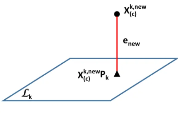
Figure 1: An illustration of OD2k in a 3-dimensional feature space.
134
space is shown in Figure 1. The new instance xk,new(c) is shown as the black
135
dot; the class subspace Lk is shown as the dark blue 2-dimensional plane;
136
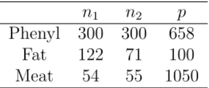
and the projection of xk,new(c) to Lk,xk,new(c) Pk, is shown as the black triangle.
137
The residual ek,new is represented by the red solid line segment, which is
138
orthogonal to the planeLk. The square of the length of the red line segment
139
is OD2k.
140
The squared score distance. The squared score distance to class k, SD2k, is
141
defined as the Mahalanobis distance from the projection of xk,new(c) to the
142
centre of the subspace Lk:
143 SD2k= rk X i=1 (tk,newi /di)2 =tk,newD−rk2(t k,new)T, (7)
where Drk is the diagonal matrix of singular values in (3). SD 2
k is the
144
reweighted squared Frobenius norm oftk,new with weights 1/di(i= 1,2, . . . , r)
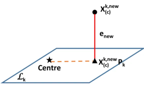
145 and 1/d1 ≤ 1/d2 ≤ . . . ≤ 1/drk. An illustration of SD 2 k in a 3-dimensional X(c) k,new Pk enew Centre Lk X(c)k,new
Figure 2: An illustration of SD2k in a 3-dimensional feature space.
146
feature space is shown in Figure 2. In addition to the symbols in Figure 1,
147
the centre of the class subspace, Lk, is shown as the black star, and the
or-148
ange dashed line connects the centre of the class subspace and the projection
149
of xk,new(c) to the class subspace. The SD2k is then the reweighted length of the
150
orange dashed line.
151
2.1.3. The classification rules
152
In NSC, the classification rule is
153
OD2k. (8)
NSC assigns xnew to the class with the smallest OD2k.
In SIMCA, a linear combination of OD2k and SD2k is often used as the 155 classification rule [2]: 156 γ ODk ck OD2 !2 + (1−γ) SDk ck SD2 !2 , (9) where γ ∈ [0,1] and ck OD2 and c k
SD2 are the cutoff values of OD 2
k and SD 2 k
157
calculated from the training set of the kth class. When γ = 1, (9) only
158
depends on OD2k, and is the same as (8) if the cutoff value ck
OD2 in (9) is one.
159
When γ = 0, (9) only depends on SD2k. In practice, the value ofγ can be set
160
by the users based on their prior knowledge of the importance of OD2k and
161
SD2k, or can be tuned by cross-validation using the training set.
162
2.2. A general formulation for the classification rules for NSM
163
Although the classification rules in NSM are in different forms, as shown
164
in (8) and (9), we shall show that they can be written using the following
165
general formulation:
166
xk,new(c) Mk1(xk,new(c) )T −tk,newMk2(tk,new)T, (10) with different Mk1 ∈Rp×p and Mk
2 ∈Rrk×rk. In this section, we derive this
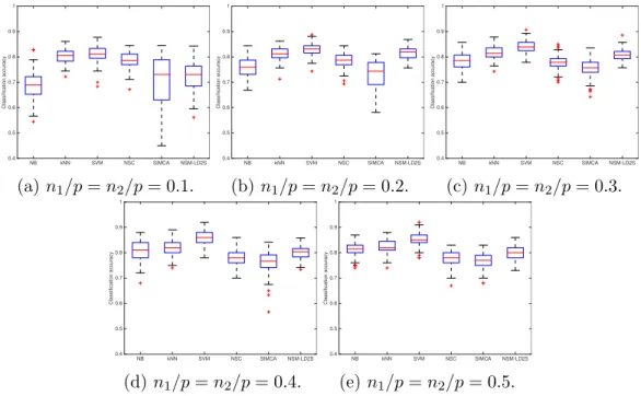
167
general formulation based on the classification rules (8) and (9), and show
168
Mk1 and Mk2 for (8) and (9), respectively. Based on the derived general
169
formulation of the classification rules, we will define the distance to subspace
170
and propose a method to learn the distance to subspace in the next section.
Substituting (6) into (5), we obtain
OD2k = (xk,new(c) −xk,new(c) Pk)(xk,new(c) −xk,new(c) Pk)T
=xk,new(c) (xk,new(c) )T −2xk,new(c) Pk(xk,new(c) )T +xk,new(c) P2k(x k,new (c) )
T
=xk,new(c) (xk,new(c) )T −xk,new(c) Pk(xk,new(c) )T
=xk,new(c) (xk,new(c) )T −tk,new(tk,new)T, (11) which indicates that OD2k is the difference between the squared Frobenius
172
norm of xk,new(c) and the squared Frobenius norm of tk,new. This is intuitive if
173
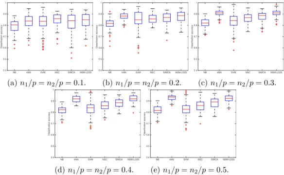
we think about the right-angled triangle formed by xk,new(c) ,xk,new(c) Pk and the
174
centre of Lk in Figure 2.
175
Then the classification rule (8) can be written as xk,new(c) (xk,new(c) )T −tk,new(tk,new)T
=xk,new(c) Mk1(N SC)(xk,new(c) )T −tk,newMk2(N SC)(tk,new)T, (12) where Mk1(N SC) = Ip and Mk2(N SC) = Irk. Equation (12) indicates that
176
the classification rule of NSC provides equal weights to the p dimensions
177
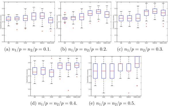
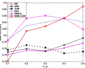
in the linear combination of the original features xk,new(c) (xk,new(c) )T and also
178
equal weights to the rk dimensions in the linear combination of the scores
179
tk,new(tk,new)T.
Similarly, for the classification rule of SIMCA, we substitute (11) to (9):
γ
(ck OD2)2
(xk,new(c) (xk,new(c) )T −tk,new(tk,new)T) + 1−γ (ck SD2)2 tk,newD−r2(tk,new)T = γ (ck OD2)2 xk,new(c) (xk,new(c) )T − r X i=1 (− 1−γ (ck SD2)2 + γ (ck OD2)2d2i )t2i
=xk,new(c) Mk1(S)(xk,new(c) )T −tk,newMk2(S)(tk,new)T, (13) where Mk1(S) = h1 1Ip,h1 = γ (ck OD2) 2 and M k
2(S) is an rk-by-rk diagonal matrix
181 with (−(c1k−γ SD2) 2 + γ (ck OD2) 2d2 i
) on the diagonals (di’s are the singular values in
182
D with d1 ≥ d2 ≥ . . . ≥ drk ≥ 0). Different from the classification rule of
183
NSM in (12), the rule in (13) indicates that the classification rule of SIMCA
184
provides equal weights to the p dimensions in the linear combination of the
185
the original featuresxk,new(c) (xk,new(c) )T, while providing different weights to the
186
rk dimensions in the linear combination of the scorestk,new(tk,new)T.
187
2.3. Learning distance to subspace
188
We define the general formulation (10) as the distance from xnew to the
189
kth class subspace. Hence we assignxnew to the nearest class subspace based
190
on the distance to subspace defined in (10).
191
The distance to subspace for the kth class defined in (10) depends on
192
two matrices: Mk1 and Mk2. It can be treated as the difference between two
193
squared distances: xk,new(c) Mk1(xk,new(c) )T is the squared distance from xk,new (c)
194
to the centre of the class subspace Lk, andtk,newMk2(tk,new)T is the squared
195
distance from the projection of xk,new(c) toLk to the centre of Lk.
196
The matrices Mk1 and Mk2 are of great importance for classification.
197
Instead of determining Mk1 and Mk2 manually as in [22] and [2], distance
metric learning methods offer us a path to learn more appropriate distance
199
metrics automatically from the training data to improve the classification
200
performance.
201
Distance metric learning methods aim to learn distance metrics based
202
on a set of similarity/dissimilarity constraints: the samples from the same
203
class should be similar while the samples from different classes should be
204
dissimilar. Thus the samples from the same class are close together while the
205
samples from different classes are farther away from each other, based on the
206
distance metric learned from the training data. In this way, the classification
207
task becomes easier and we can expect better classification performance using
208
the learned distance metrics.
209
Established distance metric learning methods are sample-based, i.e. the
210
distances that they learned are measured between samples. However, in
211
NSM, the distance is calculated between a sample and a class subspace. Thus
212
we need to develop a new method of learning the distance metric from sample
213
to subspace, to learn the distance metrics in NSM. The learned distance
214
metrics are termed “learned distance to subspace (LD2S)”. Inspired by the
215
constraints used in established distance metric learning methods, we propose
216
the following set of similarity/dissimilarity constraints for LD2S: the samples
217
should be similar to their true class while dissimilar from the wrong classes.
218
In other words, we aim to learnMk1 andMk2, such that the samples are close
219
to their true classes while farther away from the wrong classes.
220
2.3.1. Distance metric
221
In this section, we briefly review the definition of distance metric. Given a
222
set of data points {x1,x2, ...,xN}inR1×p with a set of labels{y1, y2, ..., yN},
the distance metricd(xi,xj) between two data pointsxiandxjshould satisfy
224
the following properties:
225
1. d(xi,xj)≥0 (non-negativity),
226
2. d(xi,xj) = 0 if and only if xi =xj (identity),
227
3. d(xi,xj) = d(xj,xi) (symmetry),
228
4. d(xi,xj) ≤d(xi,xk) +d(xj,xk) (triangle inequality), where xk is an
229
instance that is different to xi and xj.
230
A distance metric is known as a pseudo metric when the second property
231
is relaxed to: d(xi,xj) = 0 if xi =xj.
232
Most of the metric learning algorithms aim to learn a Mahalanobis
distance-233
like pseudo metric:
234
dM(xi,xj) =
q
(xi−xj)M(xi−xj)T, (14)
which is parameterised by M. The matrixM is set to be positive
semidefi-235
nite to ensure that dM(xi,xj) is a pseudo metric. If M is the inverse of the
236
sample variance, then dM(xi,xj) is the Mahalanobis distance. If M is the
237
identity matrix, then dM(xi,xj) is exactly the Euclidean distance.
238
2.3.2. Distance to subspace
239
Different from the distance metric between two samplesxi andxj defined
240
in (14), we define the squared distance metric between a samplexand a class
241
subspace Lk using the general formulation in (10):
242 d2(x,Lk) =xk(c)M k 1(x k (c)) T −tkMk 2(t k)T, (15)
where xk
(c) denotes the sample mean-centred by the mean of the training
243
samples of the kth class, Mk1 ∈ Rp×p is the parameterisation matrix for the
244
distance in the original feature space of thekth class,tkis the PC score of the
245
sample when projected to the PC subspace of thekth class, andMk2 ∈Rrk×rk
246
is the parameterisation matrix for the distance in the PC subspace of thekth
247
class. Then d2(x,Lk) can be treated as the difference between the squared
248
distance from the sample (column-centred by the column means of classk) to
249
the centre of Lk and the squared distance from the projection of the sample
250
to the centre of Lk.
251
2.3.3. Learned distance to subspace
252
To learn good distance metrics between samples and class subspaces, we
253
propose the following similarity/dissimilarity constraints: the samples are
254
similar to their correct class subspaces while are dissimilar to the wrong
255
class subspaces. To formulate the constraints, we define the following
simi-256
larity/dissimilarity sets:
257
S ={(xi,Lk)|xi belongs to classk}, and
258
D={(xi,Lk)|xi does not belong to classk}.
259
In the following part, the training samples from class 1 are denoted by
260
subscript 1(i), i.e.x1(i) ∈R1×pandX1 = [xT1(1), . . . ,x T 1(n1)]
T ∈
Rn1×p, and the
261
training samples from class 2 are denoted by subscript 2(j), i.e.x2(j) ∈R1×p
262
and X2 = [xT2(1), . . . ,x T 2(n2)]
T ∈
Rn2×p. Thus the similarity/dissimilarity sets
263 become 264 S ={(x1(i),L1),(x2(j),L2)|i= 1,2, . . . , n1, j = 1,2, . . . , n2}, and 265 D={(x1(i),L2),(x2(j),L1)|i= 1,2, . . . , n1, j = 1,2, . . . , n2}. 266
the sum of the distances between the samples and the class subspaces that fall into the similarity set S, while maximise the sum of those that fall into the dissimilarity setD. However, simply optimising the sums of the distances suffers from losing the information in individual samples. Hence, instead of treating all training samples together, we aim to make the difference between the distance to the wrong class and the distance to the correct class large enough for each training sample by using the following constraints:
d2(x1(i),L2)−d2(x1(i),L1)≥1, fori= 1, . . . , n1, and
d2(x2(j),L1)−d2(x2(j),L2)≥1, forj = 1, . . . , n2. (16)
In this way, the samples can be classified more easily. In addition, to en-hance the generalisation ability of the learned distance metrics, we add slack variables ξ1(i) and ξ2(j) to the constraints and aim to solve the following
op-timisation problem: min ξ1(i),ξ2(j),Mk1,Mk2 n1 X i=1 ξ1(i)+ n2 X j=1 ξ2(j) (17) s.t. d2(x1(i),L2)−d2(x1(i),L1)≥1−ξ1(i), ξ1(i) ≥0, (18) d2(x2(j),L1)−d2(x2(j),L2)≥1−ξ2(j), ξ2(j) ≥0, (19) Mk1 0 and Mk2 0, (20)
semidefi-nite. The constraints in (18) and (19) can be rewritten as
ξ1(i)≥[1 +d2(x1(i),L1)−d2(x1(i),L2)]+ and ξ2(j) ≥[1 +d2(x2(j),L2)−d2(x2(j),L1)]+,
where [l]+ = max(0, l). Hence the optimisation problem is equivalent to
min Mk 1,Mk2 n1 X i=1 [1 +d2(x1(i),L1)−d2(x1(i),L2)]++ n2 X j=1 [1 +d2(x2(j),L2)−d2(x2(j),L1)]+ s.t. Mk1 0, Mk2 0. (21) The hinge losses used in (21) only penalise the samples that do not satisfy
267
(16), while assign zero loss for the samples that satisfy (16) using NSM.
268
In this way, the hinge loss makes full use of the effectiveness of NSM. It
269
is worth noting that the hinge loss has also been popularly used in other
270
distance-based classifiers, such as support vector machine (SVM) and large
271
margin nearest neighbour (LMNN) classification [21].
272
SupposeMk∗1 and Mk∗2 (k= 1,2) denote the solutions of (21). Then the
273
learned distance from a test sample xnew to thekth class subspace is
274 d2(xnew,Lk) = xk,new(c) Mk∗1 (x k,new (c) ) T −tk,newMk∗ 2 (t k,new)T. (22)
We compared2(xnew,L1) andd2(xnew,L2), and assign xnewto the class with
275
the smallest squared distance.
276
Considering the nature of spectral data, i.e. high-dimensional feature and
small sample size, learning the full matrices, Mk1 with p(p+ 1)/2 parameters
278
andMk2 withrk(rk+ 1)/2 parameters, could easily suffer from the overfitting
279
problem. In (12) and (13), Mk1(N SC) = Ip and Mk1(S) = 1
h1Ip are identity
280
matrices with common coefficients 1 and 1/h1for all dimensions, respectively.
281
Therefore, in this paper, we learn Mk1 = ckIp(with ck ≥ 0) and Mk2 =
282
diag(mk21, mk22, . . . , mk2rk) (with each element nonnegative), as natural and
283
practically-interpretable extensions of those used in (12) and (13).
284
3. Experiments
285
In the following experiments, NSC, SIMCA and NSM with distance
mea-286
surement (22) (NSM-LD2S) are compared using high-dimensional spectral
287
data, the Phenyl dataset, the fat dataset [6] and the meat dataset [1]. We
288
also compare the classification results of the nearest subspace methods with
289
those of naive Bayes (NB), k nearest neighbours (kNN) and support vector
290
machine (SVM), to show the effectiveness of the nearest subspace methods
291
to classify high-dimensional data.
292
3.1. Datasets
293
The number of samples in each class and the number of features for the
294
three high-dimensional spectral datasets are summarised in Table 1.
295
Table 1: The number of samples in each class, n1 and n2, and the number of features p for the three high-dimensional spectral datasets.
n1 n2 p
Phenyl 300 300 658 Fat 122 71 100 Meat 54 55 1050
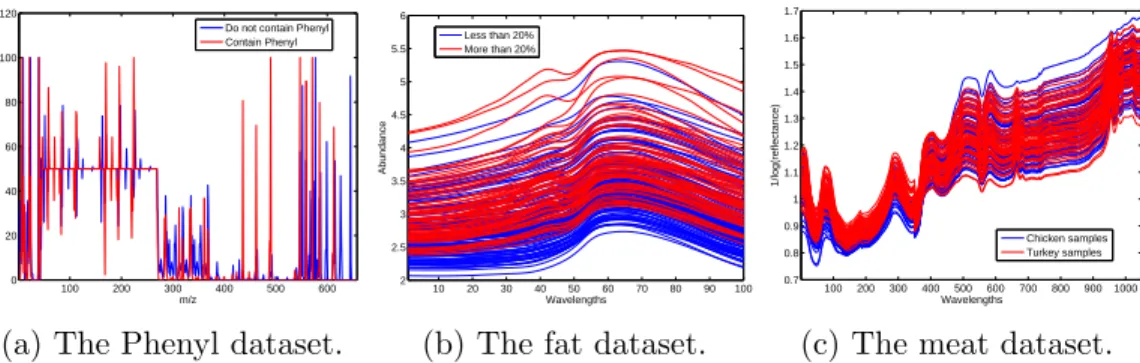
100 200 300 400 500 600 0 20 40 60 80 100 120 m/z Relative abundance
Do not contain Phenyl Contain Phenyl
(a) The Phenyl dataset.
10 20 30 40 50 60 70 80 90 100 2 2.5 3 3.5 4 4.5 5 5.5 6 Wavelengths Abundance Less than 20% More than 20%
(b) The fat dataset.
100 200 300 400 500 600 700 800 9001000 0.7 0.8 0.9 1 1.1 1.2 1.3 1.4 1.5 1.6 1.7 Wavelengths 1/log(reflectance) Chicken samples Turkey samples
(c) The meat dataset.
Figure 3: The plots of the spectra of the three datasets.
3.1.1. The Phenyl dataset
296
The Phenyl dataset is available in the ‘chemometrics’ R package, which
297
contains 300 spectra with the phenyl substructure and 300 spectra without
298
the phenyl substructure. The spectra are measured at 658 wavelengths. To
299
avoid confusing, the spectra of two instances from two classes are shown in
300
Figure 3a.
301
3.1.2. The fat dataset
302
The fat dataset contains 193 spectra of finely chopped meat, measured at
303
100 wavelengths [6]. The fat dataset consists of 122 spectra of meat samples
304
with less than 20% fat and 71 spectra of meat samples with more than 20%
305
fat. The spectra of all samples are shown in Figure 3b.
306
3.1.3. The meat dataset
307
The meat dataset [1] contains the spectra of five classes of meat
sam-308
ples, measured at 1050 wavelengths. We select the chicken and turkey meat
309
samples from the original dataset in the experiments, because they contain
310
similar chemical components and are hard to classify. The new meat dataset
contains the spectra of 55 chicken samples and the spectra of 54 turkey
sam-312
ples. The spectral of all samples are shown in Figure 3c.
313
3.2. Experiment settings
314
The classification performances of the three methods are shown for five
315
different ratios of training set size/feature dimension: n1/p = n2/p = 0.1,
316
0.2, 0.3, 0.4 and 0.5.
317
For the Phenyl dataset, we randomly select 100 samples with Phenyl
318
structure and 100 samples without Phenyl structure. For illustrative
pur-319
poses, we select the first 100 dimensions from the 658 feature dimensions for
320
the experiments in this paper, i.e. p= 100.
321
For the fat dataset, we use all the 120 meat samples with less than 20%
322
fat and 71 meat samples with more than 20% fat in the dataset. We also use
323
all the dimensions of the fat dataset, i.e. p= 100.
324
For the meat dataset, we use all the 55 chicken samples and 54 turkey
325
samples in the dataset. Again for illustrative purposes, we also select the first
326
100 dimensions from the 350 dimensions for the experiments in this paper,
327
i.e. p= 100.
328
Therefore, as p= 100 for each of the three datasets, the five training set
329
sizes are n1 = n2 = 10, 20, 30, 40 and 50. The samples to form a training
330
set are randomly selected from a dataset. The rest samples in the datasets
331
are used as test samples.
332
In NSC, SIMCA and NSM-LD2S, the numbers of PCs, rk, are tuned by
333
5-fold cross-validation using the training set to minimise the classification
334
error. More specifically, for each value of rk, we calculate the mean
classi-335
fication error of the 5-fold cross-validation. The value with the minimum
mean classification error is chosen as the number of PCs.
337
In SIMCA, ckOD = (ˆµ+ ˆσz0.975)3/2, where ˆµ and ˆσ are the mean and the
338
standard deviation of the orthogonal distances in of the training samples in
339
class k; and ckSD = qχ2
nk;0.975. The weight γ is also tuned by 5-fold
cross-340
validation using the training data.
341
In NSM-LD2S, the optimisation problem (21) is solved by ‘cvx’ in
MAT-342
LAB.
343
In SVM, the radial basis function (RBF) kernel is adopted. The scale
344
parameter of the RBF kernel and the penalty factor C are tune by 5-fold
345
cross-validation. The values of the two parameters to be chosen are set to
346
10, 102 and 103. In kNN, the number of nearest neighbours is tuned by
5-347
fold cross-validation. The values to be chosen are set to 3, 5 and 7. In NB,
348
the prior probability of each class is set as the proportion of the number of
349
training samples of that class over the total number of training samples.
350
All the random training/test splits and the subsequent experiments are
351
repeated 100 times and the classification accuracies of the test data are
352
recorded.
353
3.3. Results
354
3.3.1. The Phenyl dataset
355
The classification results of the Phenyl dataset demonstrate the superior
356
classification performance of NSM-LD2S, as shown in Figure 4 and Figure 5,
357
compared with NSC and SIMCA over all nk/p ratios. It is clear that SVM
358
performs better than the three nearest subspace methods for this dataset.
359
kNN and NB are also better than the three nearest subspace methods when
360
nk/p becomes large.
NB kNN SVM NSC SIMCA NSM-LD2S Classification accuracy 0.4 0.5 0.6 0.7 0.8 0.9 1 (a)n1/p=n2/p= 0.1. NB kNN SVM NSC SIMCA NSM-LD2S Classification accuracy 0.4 0.5 0.6 0.7 0.8 0.9 1 (b)n1/p=n2/p= 0.2. NB kNN SVM NSC SIMCA NSM-LD2S Classification accuracy 0.4 0.5 0.6 0.7 0.8 0.9 1 (c) n1/p=n2/p= 0.3. NB kNN SVM NSC SIMCA NSM-LD2S Classification accuracy 0.4 0.5 0.6 0.7 0.8 0.9 1 (d)n1/p=n2/p= 0.4. NB kNN SVM NSC SIMCA NSM-LD2S Classification accuracy 0.4 0.5 0.6 0.7 0.8 0.9 1 (e) n1/p=n2/p= 0.5.
Figure 4: Classification accuracies of NB,kNN, SVM, NSC, SIMCA and NSM-LD2S for
the Phenyl dataset.
nk/p 0.1 0.2 0.3 0.4 0.5 Mean accuracy 0.68 0.7 0.72 0.74 0.76 0.78 0.8 0.82 0.84 0.86 NB kNN SVM NSC SIMCA NSM-LD2S
Figure 5: Mean classification accuracies of NB,kNN, SVM, NSC, SIMCA and NSM-LD2S for the Phenyl dataset.
However, it is conceivable that, for certain other datasets, the
classifica-362
tion performance of NSM-LD2S cannot always be better than those of NSC
363
and SIMCA, in particular under small nk/p ratios. In the following two
364
sections, we show two examples that NSM-LD2S performs worse than NSC
365
and SIMCA for small nk/p ratios but better for large nk/p ratios. This is
366
because there are more parameters in NSM-LD2S to be learned than in NSC
367
and SIMCA, and NSM-LD2S needs more training samples to achieve good
368
classification performance for some data. In addition, the classification
per-369
formances of NB, kNN and SVM are also not always better than the nearest
370
subspace methods. The following two examples can also demonstrate this
371
argument.
372
3.3.2. The fat dataset
373
In the fat dataset, the classification performance of NSM-LD2S and SIMCA
374
are worse than NSC when nk/p = 0.1 and are better than NSC when
375
nk/p ≥ 0.2, as shown in Figure 6 and Figure 7. NSM-LD2S provides the
376
best classification performance when nk/p≥0.2.
377
It is obvious that NB has the worst mean classification accuracies for all
378
nk/pratios. kNN performs similarly to NSM-LD2S. SVM performs similarly
379
to SIMCA when nk/p = 0.1 and performs worse than the three nearest
380
subspace methods for all other nk/pratios.
381
3.3.3. The meat dataset
382
Compared with the fat dataset, the classification accuracies of the three
383
methods for the meat dataset show a stronger effect of thenk/pratios. When
384
nk/p < 0.4, NSM-LD2S performs much worse than NSC and SIMCA,
NB kNN SVM NSC SIMCA NSM-LD2S Classification accuracy 0.4 0.5 0.6 0.7 0.8 0.9 1 (a)n1/p=n2/p= 0.1. NB kNN SVM NSC SIMCA NSM-LD2S Classification accuracy 0.4 0.5 0.6 0.7 0.8 0.9 1 (b)n1/p=n2/p= 0.2. NB kNN SVM NSC SIMCA NSM-LD2S Classification accuracy 0.4 0.5 0.6 0.7 0.8 0.9 1 (c) n1/p=n2/p= 0.3. NB kNN SVM NSC SIMCA NSM-LD2S Classification accuracy 0.4 0.5 0.6 0.7 0.8 0.9 1 (d)n1/p=n2/p= 0.4. NB kNN SVM NSC SIMCA NSM-LD2S Classification accuracy 0.4 0.5 0.6 0.7 0.8 0.9 1 (e) n1/p=n2/p= 0.5.
Figure 6: Classification accuracies of NB,kNN, SVM, NSC, SIMCA and NSM-LD2S for
the fat dataset.
nk/p 0.1 0.2 0.3 0.4 0.5 Mean accuracy 0.78 0.8 0.82 0.84 0.86 0.88 0.9 0.92 0.94 NB kNN SVM NSC SIMCA NSM-LD2S
Figure 7: Mean classification accuracies of NB,kNN, SVM, NSC, SIMCA and NSM-LD2S for the fat dataset.
NB kNN SVM NSC SIMCA NSM-LD2S Classification accuracy 0.4 0.5 0.6 0.7 0.8 0.9 1 (a)n1/p=n2/p= 0.1. NB kNN SVM NSC SIMCA NSM-LD2S Classification accuracy 0.4 0.5 0.6 0.7 0.8 0.9 1 (b)n1/p=n2/p= 0.2. NB kNN SVM NSC SIMCA NSM-LD2S Classification accuracy 0.4 0.5 0.6 0.7 0.8 0.9 1 (c) n1/p=n2/p= 0.3. NB kNN SVM NSC SIMCA NSM-LD2S Classification accuracy 0.4 0.5 0.6 0.7 0.8 0.9 1 (d) n1/p=n2/p= 0.4. NB kNN SVM NSC SIMCA NSM-LD2S Classification accuracy 0.4 0.5 0.6 0.7 0.8 0.9 1 (e) n1/p=n2/p= 0.5.
Figure 8: Classification accuracies of NB,kNN, SVM, NSC, SIMCA and NSM-LD2S for
nk/p 0.1 0.2 0.3 0.4 0.5 Mean accuracy 0.72 0.74 0.76 0.78 0.8 0.82 0.84 0.86 0.88 0.9 NB kNN SVM NSC SIMCA NSM-LD2S
Figure 9: Mean classification accuracies of NB,kNN, SVM, NSC, SIMCA and NSM-LD2S for the meat dataset.
cially fornk/p= 0.1. However, whennk/p= 0.5, the classification accuracies
386
of NSM-LD2S become much better than those of NSC and SIMCA, as shown
387
in Figure 8(e) and Figure 9. The classification results of the meat dataset
388
suggest that NSM-LD2S needs nk/p > 0.4 to achieve superior classification
389
performance for the meat dataset.
390
Similarly to the fat dataset, NB and SVM have the worst classification
391
performances fornk/p >0.1 for the meat dataset. kNN performs worse than
392
the nearest subspace methods for the meat dataset.
393
3.3.4. Summary of the results
394
The experiments show that using the learned distance metrics from data
395
can provide superior classification results, compared with using
predeter-396
mined distance metrics, when the nk/pratio is large enough. For data with
397
small nk/p ratios, using the distance measurement based on LD2S may
per-398
form poorly in classification since the nk/pratio is not large enough to learn
all the parameters in LD2S.
400
It is worth noting that the nearest subspace methods are effective to
401
classify high-dimensional data. One important reason is that they find the
402
low-dimensional subspace representation for each class to extract the most
403
informative feature. Our proposed LD2S is an additional step to improve
404
the classification performance of the nearest subspace methods, based on
405
the feature-extracted data. LD2S can obtain better distance measurements
406
between a sample and a subspace, which has a positive effect on
classifi-407
cation accuracies. As demonstrated by the experiment results, NSM-LD2S
408
can achieve better classification accuracies than NSM and SIMCA, which
409
shows the effectiveness of LD2S in addition to feature extraction in NSM
410
and SIMCA.
411
4. Conclusion
412
We have proposed a general formulation of distance to subspace, i.e. the
413
distance from a sample to a PC class subspace. Based on this formulation,
414
we have proposed a simple but effective LD2S method that can learn tailored
415
distance metrics adaptively from data, for the classification rule of NSM. The
416
classification performances on three datasets demonstrate the effectiveness of
417
learning distance metrics from data when thenk/pratio is large enough. The
418
current LD2S is designed for binary classification. A multi-class version of
419
LD2S is needed for more general and practical cases and we identify this as
420
our future work.
Acknowledgement
422
The authors thank the reviewers for their constructive comments.
423
References
424
[1] T. Arnalds, J. McElhinney, T. Fearn, G. Downey, A hierarchical
dis-425
criminant analysis for species identification in raw meat by visible and
426
near infrared spectroscopy, Journal of Near Infrared Spectroscopy 12 (3)
427
(2004) 183–188.
428
[2] K. V. Branden, M. Hubert, Robust classification in high dimensions
429
based on the SIMCA method, Chemometrics and Intelligent Laboratory
430
Systems 79 (1) (2005) 10–21.
431
[3] Y. Chi, Nearest subspace classification with missing data, in: Signals,
432
Systems and Computers, 2013 Asilomar Conference on, IEEE, 2013, pp.
433
1667–1671.
434
[4] Y. Chi, F. Porikli, Connecting the dots in multi-class classification:
435
From nearest subspace to collaborative representation, in: Computer
436
Vision and Pattern Recognition (CVPR), 2012 IEEE Conference on,
437
IEEE, 2012, pp. 3602–3609.
438
[5] C. Durante, R. Bro, M. Cocchi, A classification tool for N-way array
439
based on SIMCA methodology, Chemometrics and Intelligent
Labora-440
tory Systems 106 (1) (2011) 73–85.
441
[6] F. Ferraty, P. Vieu, Nonparametric Functional Data Analysis: Theory
442
and Practice, Springer Science & Business Media, 2006.
[7] K. Fukui, A. Maki, Difference subspace and its generalization for
444
subspace-based methods, IEEE Transactions on Pattern Analysis and
445
Machine Intelligence 37 (11) (2015) 2164–2177.
446
[8] P. Hall, D. M. Titterington, J.-H. Xue, Median-based classifiers for
447
high-dimensional data, Journal of the American Statistical Association
448
104 (488) (2009) 1597–1608.
449
[9] P. Hall, J.-H. Xue, Incorporating prior probabilities into
high-450
dimensional classifiers, Biometrika 97 (1) (2010) 31–48.
451
[10] P. Hall, J.-H. Xue, On selecting interacting features from
high-452
dimensional data, Computational Statistics & Data Analysis 71 (2014)
453
694–708.
454
[11] K.-C. Lee, J. Ho, D. J. Kriegman, Acquiring linear subspaces for face
455
recognition under variable lighting, IEEE Transactions on Pattern
Anal-456
ysis and Machine Intelligence 27 (5) (2005) 684–698.
457
[12] C. Mees, F. Souard, C. Delporte, E. Deconinck, P. Stoffelen, C. St´evigny,
458
J.-M. Kauffmann, K. De Braekeleer, Identification of coffee leaves using
459
FT-NIR spectroscopy and SIMCA, Talanta 177 (2018) 4–11.
460
[13] J.-X. Mi, D.-S. Huang, B. Wang, X. Zhu, The nearest-farthest subspace
461
classification for face recognition, Neurocomputing 113 (2013) 241–250.
462
[14] B. Mnassri, B. Ananou, M. Ouladsine, et al., Fault detection and
di-463
agnosis based on PCA and a new contribution plot, IFAC Proceedings
464
Volumes 42 (8) (2009) 834–839.
[15] B. Mnassri, M. Ouladsine, et al., Reconstruction-based contribution
ap-466
proaches for improved fault diagnosis using principal component
analy-467
sis, Journal of Process Control 33 (2015) 60–76.
468
[16] I. Nejadgholi, M. Bolic, A comparative study of PCA, SIMCA and Cole
469
model for classification of bioimpedance spectroscopy measurements,
470
Computers in biology and medicine 63 (2015) 42–51.
471
[17] M. Rafferty, X. Liu, D. M. Laverty, S. McLoone, Real-time
multi-472
ple event detection and classification using moving window pca, IEEE
473
Transactions on Smart Grid 7 (5) (2016) 2537–2548.
474
[18] A. Sgarbossa, C. Costa, P. Menesatti, F. Antonucci, F. Pallottino,
475
M. Zanetti, S. Grigolato, R. Cavalli, A multivariate SIMCA index as
476
discriminant in wood pellet quality assessment, Renewable Energy 76
477
(2015) 258–263.
478
[19] Q. Tian, S. Chen, L. Qiao, Ordinal margin metric learning and its
exten-479
sion for cross-distribution image data, Information Sciences 349 (2016)
480
50–64.
481
[20] P. Van den Kerkhof, J. Vanlaer, G. Gins, J. F. Van Impe, Analysis
482
of smearing-out in contribution plot based fault isolation for statistical
483
process control, Chemical Engineering Science 104 (2013) 285–293.
484
[21] K. Q. Weinberger, L. K. Saul, Distance metric learning for large margin
485
nearest neighbor classification, Journal of Machine Learning Research
486
10 (2009) 207–244.
[22] S. Wold, Pattern recognition by means of disjoint principal components
488
models, Pattern Recognition 8 (3) (1976) 127–139.
489
[23] E. P. Xing, A. Y. Ng, M. I. Jordan, S. Russell, Distance metric learning
490
with application to clustering with side-information, Advances in Neural
491
Information Processing Systems 15 (2003) 505–512.
492
[24] J. Yu, D. Tao, J. Li, J. Cheng, Semantic preserving distance metric
493
learning and applications, Information Sciences 281 (2014) 674–686.
494
[25] L. Zhang, W.-D. Zhou, B. Liu, Nonlinear nearest subspace classifier, in:
495
International Conference on Neural Information Processing, Springer,
496
2011, pp. 638–645.
497
[26] P. Zhu, Q. Hu, W. Zuo, M. Yang, Multi-granularity distance metric
498
learning via neighborhood granule margin maximization, Information
499
Sciences 282 (2014) 321–331.
500
[27] R. Zhu, K. Fukui, J.-H. Xue, Building a discriminatively ordered
sub-501
space on the generating matrix to classify high-dimensional spectral
502
data, Information Sciences 382 (2017) 1–14.
503
[28] R. Zhu, J.-H. Xue, On the orthogonal distance to class subspaces for
504
high-dimensional data classification, Information Sciences 417 (2017)
505
262–273.