Honors Scholar Theses Honors Scholar Program Spring 6-9-2020
Applying Machine Learning to Neuroimaging Data to Identify
Applying Machine Learning to Neuroimaging Data to Identify
Predictive Models of Reading Disorder (RD)
Predictive Models of Reading Disorder (RD)
Spencer LowFollow this and additional works at: https://opencommons.uconn.edu/srhonors_theses Part of the Behavior and Behavior Mechanisms Commons
Recommended Citation Recommended Citation
Low, Spencer, "Applying Machine Learning to Neuroimaging Data to Identify Predictive Models of Reading Disorder (RD)" (2020). Honors Scholar Theses. 677.
Applying Machine Learning to Neuroimaging Data to
Identify Predictive Models of Reading Disorder (RD)
Spencer Low
Thesis submitted in partial fulfillment of the requirements for Honors in Neuroscience, University of Connecticut.
Table of Contents
Abstract
2
Introduction
4
Methods
8
1. Participants, Descriptive Statistics, and Inclusion Criteria
8
2. MRI Data
10
3. MRI Preprocessing
11
4. Multivariate Pattern Analyses
13
Results
15
Discussion
20
1. Limitations
22
2. Future Directions
23
Acknowledgements
25
References
26
Abstract
Over the last 20 years, advances in computational neuroimaging and computational power have made it feasible to create predictive models (Woo et al. Nature Neuroscience 2017). Predictive modeling is an approach that uses pattern recognition techniques (machine learning) to develop models using brain data to predict clinical (or educational) outcomes, differential diagnosis and subtyping, and inform development of new treatments (Doyle et al Royal Society 2015, Haynes Neuron 2015, Orrù et al. NBR 2012; Woo et al. Nature Neuroscience 2017). In recent years, machine learning algorithms have been implemented to develop a model (pattern classifier) using neuroimaging data to predict reading outcomes in children with a wide range of reading ability (Hoeft et al. Behav Neurosci 2007) and those diagnosed with reading disorders (RD) (Hoeft et al. PNAS 2011). In their studies, they showed that models combining
neuroimaging and behavior were superior to just behavioral measures (Hoeft et al. Behav Neurosci 2007), and that neuroimaging data was able to predict reading outcome in RD more quickly and efficiently or when behavioral measures failed to do so (Hoeft et al. PNAS 2011).
For this project, we used resting state functional MRI (rsfMRI) data coupled with multivariate pattern analysis (MVPA) to develop models that predict RD diagnosis in a large population of children. rsfMRI uses blood oxygen level dependent (BOLD) signals to provide information about functional activation and connectivity between both local and nonlocal brain regions. Through MVPA, in particular support vector machines (SVMs) and random forest classifiers, patterns of temporal connectivity that differentiate between RD and non-RD children were identified and the accuracy of the model was calculated. Further exploratory analyses are performed to identify patterns that differentiate RD and controls in younger versus older children
such that potential compensatory mechanisms and developmental differences are identified. Such tools may offer clinicians the ability to, in conjunction with behavioral techniques, more quickly and accurately diagnose children not just with RD but with a wide range of neurocognitive disorders and allow for better diagnostic criteria in the future.
Introduction
Reading disorder (RD), commonly referred to as dyslexia, occurs in about 5%-15% of school-age children (Petretto & Masala, 2017). It is marked by a persistent difficulty in the acquisition of reading skills that can’t be explained by sensory or cognitive deficits, lack of motivation, intelligence, or lack of access to instruction to reading. According to diagnostic criteria presented in the DSM-V, RD falls within the broader category of Specific Learning Disorder (American Psychiatric Association, 2013). Specific Learning Disorders are marked by three criteria: 1) the symptoms persist for greater than 6 months, 2) the impairment of one or more abilities with a prominent effect on academic performance, and 3) onset while the individual is in school (APA, 2013). Exclusion criteria include: intellectual disability,
inconsistent/insufficient education, language comprehension doesn’t allow for comprehension, and presence of sensory problems sufficient to impede upon learning (visual or auditory
problems for example) (APA, 2013). RD is specifically characterized by difficulty in acquiring and utilizing reading skills, often presenting itself during the first couple years of schooling. Diagnosis of RD through those beginning stages of schooling can be difficult. Ysseldyke and Christenson referred to a “search for pathology” when assessing the etiology of reading
difficulties as often school psychologists follow a psychometric approach to reading assessment rather than more categorical labeling (1988). For example, difficulties in reading can be caused by general intellectual defects or instructional deficits rather than a specific cognitive deficit in reading (Vellutino et al., 2004). Fish and Margolis found that of the referrals to school
psychologists, the majority were for children with reading difficulties that were serious (2 years or greater below grade level) or moderately serious (1-2 years below grade level) (1988).
Complicating this further, RD can manifest itself in different ways over the course of one’s formal education, with some individuals even learning to compensate and attain near normal reading making it incredibly difficult to diagnose behaviorally (van der Leij & van Daal, 1999, Shaywitz et al., 2003, Law et al., 2015). The future of diagnosing RD and identifying who learned to compensate may lie in the field of neuroimaging, especially in the use of MRI to identify atypicality in structural and functional networks between different brain regions. Through MRI and advanced statistical analyses, neuroscientists may be able to point to specific phonological and other deficits that constitute multifactorial liability in the reading network and be targeted during intervention (Boada et al., 2001).
Naturally, past studies have focused on the reading network as the locus of the deficits seen in RD (Kearns et al., 2019, Martin et al., 2015, Bailey et al., 2018). In the population of interest, children, the reading network consists of several areas common to both adults and children: the inferior occipital gyrus (IOG), posterior fusiform gyrus (FFG), the posterior superior temporal gyrus (STG), dorsal precentral gyrus (PCG) and other areas that are
child-specific: the intraparietal sulcus (IPS), supplementary motor area (SMA), inferior frontal gyrus pars triangularis (IFGtr), middle frontal gyrus (MFG), and thalamus (THAL) (Houdé et al., 2010, Koyama et al., 2011, Vogel et al., 2013, Murdaugh et al., 2015). These brain regions work in tandem to allow for the comprehension of lexical and sublexical phonological representation and play a role in silent articulatory processes crucial to reading (Richlan, 2012). Richlan et al. conducted a meta-analysis to investigate the functional abnormalities seen in RD (2009). Their findings demonstrate maximal underactivation in inferior parietal, superior temporal, middle and inferior temporal and fusiform regions of the left hemisphere (Richlan et al., 2009). Further
analysis of left frontal areas were characterized by underactivation in the inferior frontal gyrus, accompanied by overactivation in the primary motor cortex and the anterior insula (Richlan et al., 2009). Figure 1 was taken from Richlan’s 2009 meta-analysis which shows the regions with underactivation and overactivation.
Figure 1.“(A) Surface rendering of all 128 input foci with underactivation in red and overactivation in green. (B) Overlays of the separate ALE maps for under- (red) and overactivation (green), respectively. Regions contained in both maps are shown in yellow. (C)
Surface rendering of the difference map (after subtracting the ALE values for underactivation from the ALE values for overactivation). The blurred coloring results from discrepant activations
at surface and deeper regions. (D) Composite surface rendering of the two thresholded independent ALE maps for under- and overactivation, respectively. (E) Surface rendering of the
thresholded difference map.” (Richlan et al., 2009)
Fluent reading can be affected by disruptions in any of the previously mentioned brain regions leading to a potential RD diagnosis (Xia et al., 2017).
Previous work utilizing multi-parameter machine learning approaches to determine the neuroanatomical basis of RD have yielded promising results. Płoński et al. used a multivariate classification approach to investigate disruptions in grey matter in children with RD to see if there were interactions between regions and measures (2017). Utilizing both a 10-fold and leave-one-out cross validations, the researchers were able to classify participants at above chance accuracy (0.66 area under curve [AUC], 0.65 accuracy [ACC] and 0.65 AUC, 0.64 ACC,
respectively) into control vs. RD groups after principled feature selection (Płoński et al., 2017). These researchers then mapped the features back onto the brain and found that those that
discriminated between RD and typical development children were situated in the left hemisphere (Płoński et al., 2017). Particular regions of interest included the STG and middle temporal gyrus, subparietal sulcus (equivalent of the IPL above), and prefrontal areas (similar to PCG above), which are employed in phonological processing (Płoński et al., 2017). This corroborates findings from Raschle et al., which demonstrated reduced gray matter in left parietotemporal and
occipitotemporal areas (2011). Deficits within these areas likely lead to the sub-optimal phonological processing often seen in RD.
A machine learning approach offers an intriguing avenue to explore these multinodal disruptions between that may be the cause of RD. The approach yields a classifier that makes a determination of the category of an unknown subject - RD vs. TD for example - by examining multiregional brain areas simultaneously (Cui et al., 2016). This technique has been utilized to investigate neurological disorders such as Alzheimer’s disease, autism, and depression (Liu et al., 2014, Anderson et al., 2011, Zheng et al., 2012). This project expands upon this literature by utilizing machine learning to determine the presence of RD in a publicly available dataset.
We hypothesize that the features that differentiate between RD and TD readers will be primarily located in the left hemisphere, specifically in areas such as the temporo-parietal regions associated with phonological processing. Furthermore, we believe the binary classification models will be more accurate than the RD vs. TD classifications due to the more robust
correlations of structural and functional whole-brain connectivity during adolescence. By the end of this project, we hope to be able to make a binary age classification and correctly predict a diagnosis of RD vs. TD. Furthermore, we will create a brain growth chart to visualize the actual age against the predicted age to see if our results corroborate our hypotheses.
Methods
Figure 2.Selection of Subjects to Be Included From Total Dataset 1. Participants, Descriptive Statistics, and Inclusion Criteria
All data was collected from the publicly available dataset from the Child Mind Institute’s Healthy Brain Network project, which is a resource for research use. Figure 2 demonstrates the allocation of subjects from the project’s dataset which included 2,575 children, all of whom had
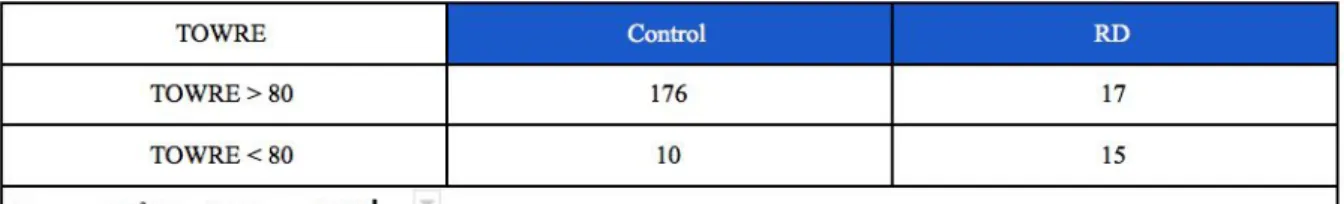
phenotypic data and 2,196 of whom had fMRI data. The phenotypic data consists of information including clinician consensus diagnoses and results of various behavioral assessments. Of these 2,575 individuals, 1,794 had fMRI data collected. To find individuals with RD, we selected subjects that had received the consensus diagnosis of RD, which was defined in the dataset as: “Specific Learning Disorder with Impairment in Reading”, N=193. From this group we excluded those with any comorbidities, giving us 33 subjects with a diagnosis of only RD. For our control population, we included only subjects who had completed all assessments and did not receive any diagnosis, giving us 249 Controls, 187 of whom had fMRI data collected. Table 1 provides the comparison between reading scores for RD vs. TD individuals with a cut off of 80 on the Test of Word Efficiency (TOWRE) scale.
Table 2 gives the demographic information for the included subjects, showing no significant differences between the Control and RD groups by age, sex, handedness, and IQ socioeconomic status.
Table 2. Demographics for Control and RD Subjects 2. MRI Data
The present project used imaging data from the Child Mind Institute - Healthy Brain
Network Network project. “Imaging data was collected using a Siemens 3 T Tim Trio MRI
scanners located at the Rutgers University Brain Imaging Center (RUBIC) and HBN (Healthy
was selected based on physical proximity to the HBN Diagnostic Research Center in Staten
Island, New York (12.7 miles; average ride duration: 24 min). The systems are equipped with a Siemens 32-channel head coil and the CMRR simultaneous multi-slice echo planar imaging
sequence. When possible, the structural and functional MRI scan parameters were selected to
facilitate harmonization with the recently launched NIH ABCD Study (this was not possible for
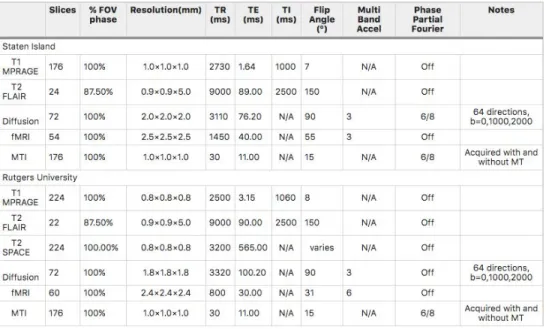
the diffusion imaging due to limitations of the Trio platform).” (Alexander et al., 2017). Parameters for the two machines are given in Table 3.
Table 3. MRI parameters for the two scanners used for data collection (Alexander et al., 2017)
3. MRI Preprocessing
Subjects anatomical and functional resting state brain data were visually examined for motion artifacts. Subjects that did not have resting state data were removed from the data set. To confirm visual inspection was sufficient MRIQC (magnetic resonance imaging quality control) software was used to quantitatively determine which subjects to exclude due to poor imaging
dataset examined by MRI experts that denotes if a subjects’ scans are accepted or rejected based on the quality of the metric reports (Esteban et. al., 2019). Upon comparison with visual
inspection, MRIQC rejected one RD scan that was initially accepted visually, while visual inspection rejected two RD scans that MRIQC accepted. It was decided that only those scans accepted by MRIQC would be included in data analysis. To assess the quality of the functional scans, the Artifact Detection (ART) Toolbox was used (citation needed). Due to children being more likely than adults to have in-scanner movement, the liberal settings in ART toolbox were used. Subjects with greater than ⅓ of their total scans flagged by the ART toolbox were excluded from the final analysis. After excluding for lack of resting state scans and MRIQC and ART Toolbox exclusion criteria, there were 28 controls and 4 RD subjects excluded.
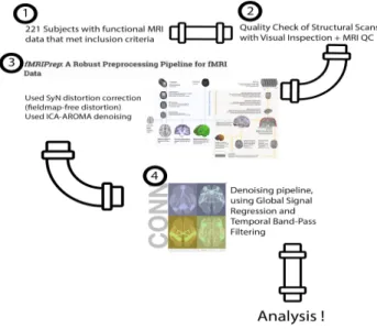
After identification of the subjects, the corresponding MRI data was preprocessed using the FMRIprep pipeline. FMRIprep is a new pipeline that “integrates the best-in-breed tools for each of the preprocessing tasks that the workflow covers” (Esteban et. al., 2019). HealthyMinds provides the neuroimaging data in Brain Imaging Data Structure (BIDS) format, which is a requirement for FMRIprep pipeline.Due to missing data within the dataset and to maintain preprocessing consistency, the flag “--ignore fieldmaps” was used. After preprocessing the MRI data, only subjects that were able to be successfully pre-processed and met quality control standards were included. After running FMRIprep, 41 Controls and 1 RD were excluded due to pre-processing errors (i.e. improper formatting, missing files, etc.). This left us with a final set of 118 controls and 29 RD for analysis. Figure 3 provides a visual for the preprocessing pipeline.
Figure 3. A visual representation of the preprocessing pipeline. After assessing initial inclusion criteria, 221 subjects remained. We then proceeded to run MRI quality control in conjunction with visual inspection and fMRIPrep to prepare our data for analysis.
4. Multivariate Pattern Analyses
After these exclusions, the data was prepared to be analyzed using linear SVMs, random forest models, and linear SVR using scikit-learn, a free Python based machine learning library (Pedregosa et al., 2011). Figure 4 provides a visual description of the data analysis pipeline.
Figure 4. Step one of analysis created the connectivity matrices through creation of a table of all the
connections for each of the subjects. Step 2 was
implementing a PCA approach to reduce the number of features before implementing SVM and SVR in step 3.
In order to extract the features most important in guiding the models, we used ROIs derived from the 100-area parcellation in Schaefer et al. (2017)First, the
global BOLD time-series for each subject’s ROIs, where the subject’s data and ROI parcellation maps are both in MNI space (Esteban et al., 2019) using the CONN toolbox Whitfield-Gabrieli & Nieto-Castanon, 2012). Our training features consisted of the resulting 4,950 total
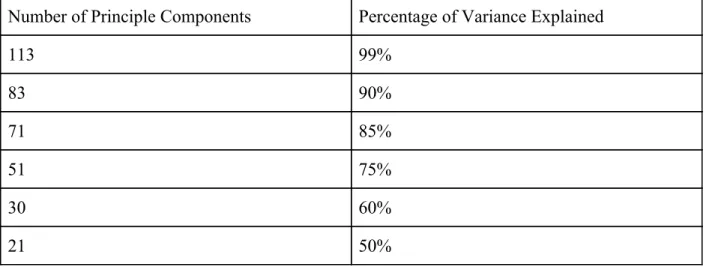
non-redundant pairwise connections between all 100 ROIs (Schaefer et al., 2017). We then implemented Principal Component Analysis (PCA) to reduce our total number of training features from 4,950 to a smaller number of features that maintained different percentages of the variance to reduce computational resources (Table 4). (Schaefer et al., 2017).
Number of Principle Components Percentage of Variance Explained
113 99% 83 90% 71 85% 51 75% 30 60% 21 50%
Table 4. Variance in the Dataset Explained by Number of Principle Components Used. In order to reduce computational resources and potentially remove noise, PCA was implemented
to reduce the number of features the machine learning classifiers are trained on from the 4,950 pairwise connections between all 100 ROIs to 21-113 features depending on the number of
principle components used.
After generation of the RRMs for the 147 subjects (118 controls and 29 RDs), we proceeded to carry out a binary categorical diagnosis classification, separating a typical
development (TD) subject with no diagnosis from a subject with reading disorder (RD). For this purpose an support vector machine (SVM) and random forest classifier were trained using the pairwise connections between ROIs and each of the PCs listed in Figure 5 as the features and
categorical diagnosis as the training parameter (class label), utilizing a grid-search to optimize the model hyperparameters and the leave-one-out cross validation method to maximize dataset usage. After calculating the accuracy, sensitivity, and specificity of our trained model, we then calculated odds ratio as well as the positive and negative likelihood ratios to determine the significance of the models.
Results:
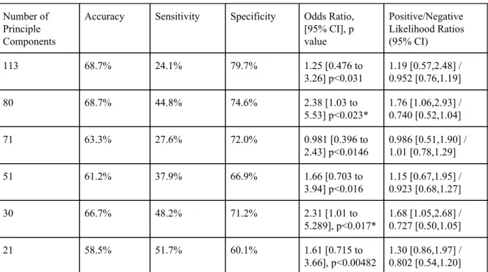
After implementation of the SVM model with gridsearch for best hyperparameters for TD/RD prediction for each number of PCs, we found two models reached a threshold of
significance (Table 5). At 83 PCs, the model’s odds ratio, a measure that determines the amount of association between two events, is 2.38 (95% CI, 1.03, 5.53; p<0.023). At 30 PCs with the default kernel and no gridsearch the model returned an odds ratio of 2.31 (95% CI, 1.01, 5.29; p<0.017). Any odds ratio greater than one implies there is a correlation between these two events, making both models significant. In both cases, the confidence interval doesn’t cross the threshold of 1, further corroborating the significance of these models. Furthermore the positive likelihood ratio, the ratio between the number of true positives and false positives is greater than 1, 1.76 and 1.68 for 83 and 30 PCs respectively, which is an important factor to determine accuracy.
Number of Principle Components
Accuracy Sensitivity Specificity Odds Ratio,
[95% CI], p value Positive/Negative Likelihood Ratios (95% CI) 113 68.7% 24.1% 79.7% 1.25 [0.476 to 3.26] p<0.031 1.19 [0.57,2.48] / 0.952 [0.76,1.19] 80 68.7% 44.8% 74.6% 2.38 [1.03 to 5.53] p<0.023* 1.76 [1.06,2.93] / 0.740 [0.52,1.04] 71 63.3% 27.6% 72.0% 0.981 [0.396 to 2.43] p<0.0146 0.986 [0.51,1.90] / 1.01 [0.78,1.29] 51 61.2% 37.9% 66.9% 1.66 [0.703 to 3.94] p<0.016 1.15 [0.67,1.95] / 0.923 [0.68,1.27] 30 66.7% 48.2% 71.2% 2.31 [1.01 to 5.289], p<0.017* 1.68 [1.05,2.68] / 0.727 [0.50,1.05] 21 58.5% 51.7% 60.1% 1.61 [0.715 to 3.66], p<0.00482 1.30 [0.86,1.97] / 0.802 [0.54,1.20]
Table 5. Results of SVM Models for RD/TD Prediction for each Number of PC’s After Gridsearch for Best Hyperparameters
(* significant at p < 0.05)
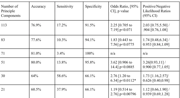
We then proceeded to run models for RD vs. TD using Random Forest Models at the same number of PCs using gridsearch to verify the hyperparameters as seen in Table 6. Under these conditions, only the 30 PC model was significant with an odds ratio of 2.76 (95% CI, 1.20, 6.34; p<0.011). Accuracy, sensitivity, and specificity were all above the threshold of chance as well. In the 30 PC case, the model also had a positive likelihood ratio of 1.73 to further support the findings.
Number of Principle Components
Accuracy Sensitivity Specificity Odds Ratio, [95%
CI], p value Positive/Negative Likelihood Ratios (95% CI) 113 76.9% 17.2% 91.5% 2.25 [0.705 to 7.19] p<0.071 2.03 [0.75,5.50] / .904 [0.76,1.08] 83 77.6% 10.3% 94.1% 1.83 [0.443 to 7.56] p<0.0775 1.74 [0.48,6.34] / 0.953 [0.84,1.09] 71 81.0% 3.4% 100% n/a n/a 51 80.0% 13.8% 95.8% 3.62 [0.906 to 14.4] p<0.0885 3.26[0.93,11] / 0.900 [0.77,1.05] 30 64% 58.6% 66.1% 2.76 [1.20 to 6.34] p<0.0112* 1.73 [1.16,2.57]/ 0.626 [0.40,0.98] 21 60.5% 37.9% 66.1% 1.19 [0.514 to 2.76] p<0.00796 1.12 [0.66,1.90] / 0.939 [0.69,1.28]
Table 6. Results of Random Forest Models for RD/TD Prediction for each Number of PC’s After Gridsearch for Best Hyperparameters
(* significant at p < 0.05)
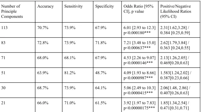
We then shifted our attention to binary age prediction using the same tools as before. First we utilized gridsearch at the same numbers of PCs as above and created SVM models for each. Table 7 demonstrates that each of the models were significant, but the 83 PC model had the best accuracy, sensitivity, and specificity as well as the best odds ratio of 7.21 (95% CI, 3.48, 15.0; p<0.00001). In comparison to the RD/TD comparison, the positive likelihood was also higher suggesting that the resting state fMRI data were much more effective for binary age classification using 10 as the arbitrary cutoff.
Number of Principle Components
Accuracy Sensitivity Specificity Odds Ratio [95%
CI], p value Positive/Negative Likelihood Ratios (95% CI) 113 70.7% 73.9% 67.9% 6.01 [2.93 to 12.3] p<0.000180*** 2.31[1.62,3.28] / 0.384 [0.25,0.59] 83 72.8% 73.9% 71.8% 7.21 [3.48 to 15.0] p<0.000637*** 2.62[1.79,3.84] / 0.363 [0.24,0.55] 71 68.0% 68.1% 67.9% 4.53 [2.26 to 9.07] p<0.0000146*** 2.13[1.26,2.05] / 0.469[0.20,0.63] 51 63.9% 81.2% 48.7% 4.09 [1.93 to 8.66] p<0.0000987*** 1.583[1.24,2.02] / 0.387[0.23,0.66] 30 68.7% 73.9% 64.1% 5.06 [2.49 to 10.3] p<0.0000415*** 2.06[1.48, 2.86] / 0.407[0.26,0.63] 21 66.0% 71.0% 61.5% 3.92 [1.97 to 7.83] p<0.00000175*** 1.85[1.34,2.54] / 0.471[0.31,0.71]
Table 7. Results of SVM Models for Binary Age Prediction (less than 10 or 10 and older) for each Number of PC’s After Gridsearch for Best Hyperparameters
(*** significant at p < 0.001)
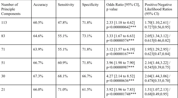
Next, we implemented the same random forest classifier for binary age prediction again using gridsearch to determine the best parameters utilizing the same PCs as before. Again, all the models created were significant but in this case the 30 PC model had the best accuracy,
sensitivity, and specificity as shown in Table 8. Furthermore, the odds ratio of 4.27 (95% CI, 2.14, 8.52; p<0.00001 suggests high significance of this particular model. The high positive likelihood ratio corroborates this information.
Number of Principle Components
Accuracy Sensitivity Specificity Odds Ratio [95% CI], p value Positive/Negative Likelihood Ratios (95% CI) 113 60.5% 47.8% 71.8% 2.33 [1.18 to 4.62] p<0.000000642*** 1.70[1.10,2.61] / 0.727[0.56,0.95] 83 64.6% 55.1% 73.1% 3.33 [1.67 to 6.63] p<0.00000574*** 2.05[1.34,3.12] / 0.615[0.46,0.82] 71 63.9% 55.1% 71.8% 3.12 [1.57 to 6.19] p<0.00000167*** 1.95[1.29,2.95] / 0.623[0.47,0.84] 51 66.7% 60.9% 71.8% 3.96 [1.98 to 7.90] p<0.00000987*** 2.16[1.44,3.22] / 0.545[0.39,0.75] 30 67.3% 68.1% 66.7% 4.27 [2.14 to 8.52] p<0.00000636*** 2.04[1.44,3.06] / 0.478[0.35,0.70] 21 66.0% 71.0% 61.5% 3.92 [1.96 to 7.83] p<0.000001748*** 1.51[1.07,2.13] / 0.68[0.49,0.95]
Table 8. Results of Random Forest Models for Binary Age Prediction (less than 10 or 10 and older) for each Number of PC’s After Gridsearch for Best Hyperparameters
(*** significant at p < 0.001)
Following the SVM and random forest models for RD vs. TD and binary age prediction, a growth chart was created using 29 PC SVR (Figure 5). A logarithmic function was fit to the data to determine where participants' actual age fell in comparison to their predicted age with the logarithmic function serving as the hyperplane divider. Fifteen of the twenty-nine (51.7%) of the RD participants fell below the growth curve.
Figure 5.Brain Growth Chart Created Using 29 PC SVR. Red=TDs, Blue=RDs. Logarithmic function fit to data to create a growth curve.
Discussion:
For both RD vs. TD and binary age prediction, SVM models and random forest models were able to determine which subjects belonged to each category with significance. In the RD vs. TD models, this could only be done at certain PCs. This may be because the PCA is designed to reduce dimensions and reduce computational stress but may have also incidentally removed noise from the data that allowed for improved classification as the PCs do not account for all variance of network data. At too many PCs, the noise from the rest of the brain may have prevented the model from choosing the features that were most important to determining if the participant had RD or not. At too few PCs, the model may not have had enough features to
accurately predict which group the subject belonged to. Thus the accuracy, sensitivity, and specificity of the model fell. This might account for the discrepancies between the different models.
For the binary age prediction models, both SVM models and random forest models were significant at all combinations of PCs. In this case, the differences in brain structure between adolescence and childhood could have allowed the model to properly classify age at different levels of variance (different numbers of PCs). Literature suggests that adolescence starts at the age of 10 (Arain et al., 2013). With adolescence comes a host of factors that influence thinking such as hormonal surges, sex hormones such as testosterone, estrogen, and progesterone, etc. (Arain et al., 2013). Onset of adolescence triggers a series of physiological changes that physically alter the structure of our brains (Arain et al., 2013). These alterations appear to be significant enough for the SVM models and the random forest classifier to detect despite any variation in noise that comes from changing the number of PCs being analyzed. In addition, the significance of the model takes on greater weight when considering the phenotypic data did not explicitly say that the ages recorded were the days the subject’s fMRI scans were conducted. Moreover, the cut-off at the age of 10 created granular separation of subjects in some cases. For example, there was one subject in the child group whose listed age was 9.87 years and another subject in the adolescent group whose listed age was 10.21. The difference between the two is miniscule so the ability of the model to make predictions on the entire dataset with significance speaks to the ability of the models to effectively use the data to find signals for classification.
The SVR generated growth chart exhibits the functional connectivity of subjects as they age using a fitted logarithmic function. The blue indicates RD subjects. Fifteen of the
twenty-nine clinician-diagnosed subjects (51.7%) fell below the growth curve indicating a younger predicted brain age than actual age. A potential explanation for those that fell above the growth curve can be provided through compensation theory in RD. Pugh et al., found that reading-impaired individuals demonstrated greater reliance on inferior frontal and right hemisphere posterior regions (2001). They proposed that this heightened reliance was in
compensation for the posterior left hemisphere difficulties in reading comprehension (Pugh et al., 2001). This increased connectivity may have confounded the model causing the fourteen
individuals to fall above the growth curve as seen in Figure 10.
Limitations:
A caveat to our results were discrepancies in diagnosis. We took the clinician consensus diagnosis as an RD diagnosis, but RD is notoriously difficult to diagnose behaviorally
(Ozernov-Palchik et al., 2017). Aaron et al. suggest that conventional measures of diagnosing RD often overlap with ADHD diagnosis, making the clinician’s task even more difficult (2002). Moreover, instead of creating an arbitrary cutoff for determining RD vs. TD, we chose to use clinician consensus diagnosis provided in the phenotypic data. This led to ten participants being in the TD group with TOWRE scores one standard deviation lower than the typical reading disorder cut-off (<90) found in the literature and fifteen subjects in the RD group with TOWRE scores higher than 90 (Nugiel et al., 2019). In future work, the researchers should create a
standardized measure of diagnosing RD, whether that be through task-based behavioral measures or through neuropsychological testing such as TOWRE-2, Comprehensive Test of Phonological Processing (CTOPP), Wechsler Intelligence Scale for Children (WISC), etc. (Hamilton &
Glascoe, 2006). With that said, the researchers must take care to choose the correct test to ensure the best results possible.
Secondly, the sample included participants (1 RD and 1 TD) with below-average IQs (75 [less than 1.5 standard deviations below the norm of 100]) which may have acted as a confound to the RD diagnosis. As mentioned above, one of the exclusion criteria for RD is intellectual disability and IQ deviation greater than 1.5 derivations could fall under the classification of intellectual disability. For greater clarity, investigators should provide a standardized number as a cut-off for IQ scores to prevent inclusion of those that may have intellectual disability.
The dataset also included children as young as 5 years old. Neuropsychological testing such as TOWRE-2 youngest standardized scores only go as low as 6 years old so the 5 year olds included in the dataset could not be properly evaluated. Typically, RD is diagnosed clinically between second grade to fourth grade (ages 7-9) so there may have been younger children who belonged in the RD group but were unable to be diagnosed due to limitations in behavioral and neuropsychological testing.
Future Directions:
Using this data, further exploratory analyses should be considered to determine
mechanisms of compensation through patterns of neural activity and connectivity in children vs. adolescents. A “child” is defined as within the age range from 5-9, while the definition of “adolescent” is derived from the World Health Organization as within the age range of 10-21. Compensation is generally seen as an individual enters adolescence (Shaywitz et al., 2002, Hancock et al., 2017). Determining which brain regions are associated with compensation could guide interventions to focus on improving these particular areas. We suggest that further research
be done into compensation and how therapy and treatment can improve outcomes in person with an RD diagnosis.
On a larger scale, it is critical to make this technology more accessible to clinicians and patients to improve diagnostic time. In some cases, it can take multiple years for behavioral observations to result in the correct diagnosis of RD (Lyon, 1996). Turning to fMRI and machine learning would drastically curb the waiting time on a correct diagnosis. The easiest method would be to follow a similar methodology as the Healthy Minds Institute by testing as many people as possible (Healthy Brain Network). Not only would this provide a larger dataset for researchers to work with, participants would be able to receive interventions earlier and
potentially learn methods of compensation improving their own quality of life. Eventually, when fMRI methods have sufficiently improved to provide high accuracy machine learning models, these techniques may be used in conjunction with more cost-effective techniques such as EEG. When used in combination with traditional methods such as clinician input and behavioral assessments, it offers hope for the future of diagnosing neurological disorders such as RD.
Acknowledgements:
I would like to express my appreciation for Dr. Fumiko Hoeft for inviting me into
BrainLENS when I approached her as a potential individualized major advisor and giving me the opportunity to explore the world of fMRI and machine learning. She matched me up to a project that expanded my academic horizons and armed me with the tools to take the next steps in my future.
I would also like to extend genuine thanks to Shaan Kamal, a 3rd year medical student at UConn Health, for his time and energy on both the project and the many lessons he taught me along the way, both within the laboratory and outside of it. Your willingness to meet me where I was at and coach me along made this project as enjoyable as possible. I can’t even begin to express how much your guidance and encouragement meant to me.
My gratitude also extends to my laboratory colleagues on this project: Oliver McNeil and Natasza Marrouch. Their work was instrumental in developing the project and I wish them many successes in the future.
Lastly, I would like to thank Dr. Blair Johnson and Dr. Rebecca Acabchuk from the SHARP laboratory for instilling a love of research and providing a gentle nudge to join Dr. Hoeft’s laboratory after hearing about my interest in neuroimaging. Furthermore, I would also like to thank Dr. Johnson for agreeing to be the second reader for this thesis.
References:
Aaron, P. G., Joshi, R. M., Palmer, H., Smith, N., & Kirby, E. (2002). Separating genuine cases of reading disability from reading deficits caused by predominantly inattentive ADHD behavior. Journal of Learning Disabilities, 35(5), 425–436.
Alexander, L. M., Escalera, J., Ai, L., Andreotti, C., Febre, K., Mangone, A., Vega-Potler, N., Langer, N., Alexander, A., Kovacs, M., Litke, S., O’Hagan, B., Andersen, J., Bronstein, B., Bui, A., Bushey, M., Butler, H., Castagna, V., Camacho, N., … Milham, M. P. (2017). Data Descriptor: An open resource for transdiagnostic research in pediatric mental health and learning disorders. Scientific Data, 4(1), 1–26.
American Psychiatric Association. (2013). Specific Learning Disorder. In Diagnostic and
Statistical Manual of Mental Disorders(5th ed.).
Arain, M., Haque, M., Johal, L., Mathur, P., Nel, W., Rais, A., Sandhu, R., & Sharma, S. (2013). Maturation of the adolescent brain. In Neuropsychiatric Disease and
Treatment(Vol. 9, pp. 449–461).
Anderson, J. S., Nielsen, J.A., Froehlich, A. L., DuBray, M. B., Druzgal, T. J., Cariello, A. N., Cooperrider, J. R., Zielinski, B. A., Ravichandran, C., Fletcher, P. T., Alexander, A. L., Bigler, D. D., Lange, N., Lainhart, J. E., (2011). Functional connectivity magnetic resonance imaging classification of autism, Brain, 134(12) 3742–3754.
Bailey, S. K., Aboud, K. S., Nguyen, T. Q., & Cutting, L. E. (2018). Applying a network framework to the neurobiology of reading and dyslexia. Journal of
Neurodevelopmental Disorders, 10(1).
Boada, R., Tunick, R. A., Olson, R. K., Willcutt, E. G., Pennington, B. F., & Ogline, J. S. (2001). A Comparison of the Cognitive Deficits in Reading Disability and
Attention-Deficit/Hyperactivity Disorder. Journal of Abnormal Psychology, 110(1). Cui, Z., Xia, Z., Su, M., Shu, H., & Gong, G. (2016). Disrupted white matter connectivity
underlying developmental dyslexia: A machine learning approach. Human Brain
Mapping, 37(4), 1443–1458.
Fish, M. C., & Margolis, H. (1988). Training and practice of school psychologists in reading assessment and intervention. Journal of School Psychology, 26(4), 399–404.
Hamilton, S. S., & Glascoe, F. P. (2006). Evaluation of children with reading difficulties.American Family Physician, 74(12), 2079-2086.
Hancock, R., Richlan, F., & Hoeft, F. (2017). Possible roles for fronto-striatal circuits in reading disorder. Neuroscience and Biobehavioral Reviews, 72, 243–260).
Healthy Brain Network - The Healthy Brain Network is a landmark mental health study that
will help children in New York City and around the world.(n.d.). Retrieved May 16,
2020, from https://healthybrainnetwork.org/
Hoeft, F., McCandliss, B. D., Black, J. M., Gantman, A., Zakerani, N., Hulme, C., Lyytinen, H., Whitfield-Gabrieli, S., Glover, G. H., Reiss, A. L., & Gabrieli, J. D. E. (2011). Neural systems predicting long-term outcome in dyslexia. Proceedings of the National
Academy of Sciences of the United States of America, 108(1), 361–366.
Houdé, O., Rossi, S., Lubin, A., & Joliot, M. (2010). Mapping numerical processing, reading, and executive functions in the developing brain: An fMRI meta-analysis of 52 studies including 842 children. Developmental Science, 13(6), 876–885.
Kearns, D. M., Hancock, R., Hoeft, F., Pugh, K. R., & Frost, S. J. (2019). The Neurobiology of Dyslexia. TEACHING Exceptional Children, 51(3), 175–188.
Koyama, M. S., di Martino, A., Zuo, X. N., Kelly, C., Mennes, M., Jutagir, D. R., Castellanos, F. X., & Milham, M. P. (2011). Resting-state functional connectivity indexes reading competence in children and adults. Journal of Neuroscience, 31(23), 8617–8624. Law, J. M., Wouters, J., & Ghesquière, P. (2015). Morphological Awareness and Its Role in
Compensation in Adults with Dyslexia. Dyslexia, 21(3), 254–272.
Liu, F., Wee, C. Y., Chen, H., & Shen, D. (2014). Inter-modality relationship constrained multi-modality multi-task feature selection for Alzheimer’s Disease and mild cognitive impairment identification. NeuroImage, 84, 466–475.
Lyon, G. (1996). Learning Disabilities. The Future of Children,6(1), 54-76.
Martin, A., Schurz, M., Kronbichler, M., & Richlan, F. (2015). Reading in the brain of children and adults: A meta-analysis of 40 functional magnetic resonance imaging studies. Human Brain Mapping, 36(5), 1963–1981.
Murdaugh, D. L., Maximo, J. O., & Kana, R. K. (2015). Changes in intrinsic connectivity of the brain’s reading network following intervention in children with autism. Human
Brain Mapping, 36(8), 2965–2979.
Nugiel, T., Roe, M. A., Taylor, W. P., Cirino, P. T., Vaughn, S. R., Fletcher, J. M., Juranek, J., & Church, J. A. (2019). Brain activity in struggling readers before intervention relates to future reading gains. Cortex, 111, 286–302.
Ozernov-Palchik, O., Norton, E. S., Sideridis, G., Beach, S. D., Wolf, M., Gabrieli, J. D. E., & Gaab, N. (2017). Longitudinal stability of pre-reading skill profiles of kindergarten children: implications for early screening and theories of reading. Developmental
Science, 20(5).
Pedregosa, F., Varoquaux, G., Gramfort, A., Michel, V., Thirion, B., Grisel, O., Blondel, M., Prettenhofer, P., Weiss, R., Dubourg, V. Vanderplas, J., Passos, A., Cournapeau, D., Brucher, M. Perrot, M., Duchesnay, E. (2011). Scikit-learn: Machine Learning in Python. Journal of Machine Learning Research, 12, 2825-2830.
Petretto, D. R., & Masala, C. (2017). Dyslexia and Specific Learning Disorders: New International Diagnostic Criteria. Journal of Childhood & Developmental Disorders,
03(04).
Płoński, P., Gradkowski, W., Altarelli, I., Monzalvo, K., van Ermingen-Marbach, M., Grande, M., Heim, S., Marchewka, A., Bogorodzki, P., Ramus, F., & Jednoróg, K. (2017). Multi-parameter machine learning approach to the neuroanatomical basis of developmental dyslexia. Human Brain Mapping, 38(2), 900–908.
Pugh, K. R., Mencl, W. E., Jenner, A. R., Katz, L., Frost, S. J., Lee, J. R., Shaywitz, S. E., & Shaywitz, B. A. (2001). Neurobiological studies of reading and reading disability.
Journal of Communication Disorders, 34(6), 479–492.
Raschle, N. M., Chang, M., & Gaab, N. (2011). Structural brain alterations associated with dyslexia predate reading onset. NeuroImage, 57(3), 742–749.
Richlan, F., Kronbichler, M., & Wimmer, H. (2009). Functional abnormalities in the dyslexic brain: A quantitative meta-analysis of neuroimaging studies. Human Brain
network. Frontiers in Human Neuroscience, 6, 120.
Shaywitz, B. A., Shaywitz, S. E., Pugh, K. R., Mencl, W. E., Fulbright, R. K., Skudlarski, P., Constable, R. T., Marchione, K. E., Fletcher, J. M., Lyon, G. R., & Gore, J. C. (2002). Disruption of posterior brain systems for reading in children with developmental dyslexia. Biological Psychiatry, 52(2), 101–110.
Shaywitz, S. E., Shaywitz, B. A., Fulbright, R. K., Skudlarski, P., Mencl, W. E., Constable, R. T., Pugh, K. R., Holahan, J. M., Marchione, K. E., Fletcher, J. M., Lyon, G. R., & Gore, J. C. (2003). Neural systems for compensation and persistence: Young adult outcome of childhood reading disability. Biological Psychiatry, 54(1), 25–33. van der Leij, A., & van Daal, V. H. (1999). Automatization aspects of dyslexia: speed
limitations in word identification, sensitivity to increasing task demands, and orthographic compensation. Journal of Learning Disabilities, 32(5), 417–428. Vellutino, F. R., Fletcher, J. M., Snowling, M. J., & Scanlon, D. M. (2004). Specific reading
disability (dyslexia): What have we learned in the past four decades? Journal of
Child Psychology and Psychiatry and Allied Disciplines, 45(1), 2-40.
Vogel, A. C., Church, J. A., Power, J. D., Miezin, F. M., Petersen, S. E., & Schlaggar, B. L. (2013). Functional network architecture of reading-related regions across development.
Brain and Language, 125(2), 231–243.
Whitfield-Gabrieli, S., & Nieto-Castanon, A. (2012). Conn: A functional connectivity toolbox
for correlated and anticorrelated brain networks. Brain connectivity, 2(3), 125-141. Xia, Z., Hancock, R., & Hoeft, F. (2017). Neurobiological bases of reading disorder Part I:
Etiological investigations. Language and Linguistics Compass, 11(4).
Ysseldyke, J. E., & Christenson, S. L. (1988). Linking assessment to intervention: Enhancing instructional options for all students. National Association of School
Psychologists, 91-109.
Zeng, L., Shen, H., Liu, L., Wang, L., Li, B., Fang, P., Zhou, Z., Li, Y., Hu, D., (2012). Identifying major depression using whole-brain functional connectivity: a multivariate pattern analysis, Brain 135(5), 1498–1507