Multiple Kernel Learning and Feature Space Denoising
FEI YAN JOSEF KITTLER KRYSTIAN MIKOLAJCZYK
Centre for Vision, Speech and Signal Processing, University of Surrey Guildford, Surrey, GU2 7XH, UK
E-MAIL:{f.yan, j.kittler, k.mikolajczyk}@surrey.ac.uk
Abstract
We review a multiple kernel learning (MKL) tech-nique called`p regularised multiple kernel Fisher dis-criminant analysis (MK-FDA), and investigate the ef-fect of feature space denoising on MKL. Experiments show that with both the original kernels or denoised ker-nels, `p MK-FDA outperforms its fixed-norm counter-parts. Experiments also show that feature space denois-ing boosts the performance of both sdenois-ingle kernel FDA and`pMK-FDA, and that there is a positive correlation between the learnt kernel weights and the amount of variance kept by feature space denoising. Based on these observations, we argue that in the case where the base feature spaces are noisy, linear combination of kernels cannot be optimal. An MKL objective function which can take care of feature space denoising automatically, and which can learn a truly optimal (non-linear) combi-nation of the base kernels, is yet to be found.
Keywords:
Kernel Methods, Multiple Kernel Learning, Kernel FDA, Kernel PCA
1
Introduction
Kernel methods [11, 13] have proven successful for many machine learning problems since their introduction in the mid-1990s. Representative methods such as support vector machine (SVM) [16, 13], kernel Fisher discriminant analysis (kernel FDA) [9, 2], kernel principal component analysis (kernel PCA) [12] have been reported to produce the state-of-the-art performance in numerous applications. Kernel methods work by embedding data items in an input space (vector, graph, string, etc.) into a vector space called a feature space, and applying linear methods in such a feature space. This embedding is defined implicitly by specifying an inner product for the feature space via a positive semidef-inite (PSD) kernel function:k(xi,xj) =< φ(xi), φ(xj)>,
wherexiandxjare two data items in the input space, and φ(·)is the (implicit) mapping function.
In kernel methods, the choice of kernel function is criti-cally important, since it completely determines the embed-ding of the data in the feature space. In many problems, multiple kernels capturing different “views” of the problem are available. In such a situation, one naturally wants to combine these kernels in an “optimal” way. This multiple kernel learning (MKL) problem was pioneered by Lancriet et al. in [8], where the key idea is to learn a linear com-bination of a given set of base kernels by maximising the (soft) margin between two classes or by maximising kernel alignment. Following this seminal work, MKL has become one of the most active areas in the machine learning com-munity in the past few years. Various extensions have been made to [8]. For example, the efficiency of MKL is signif-icantly improved in [1, 14, 10]; multiclass and multilabel MKL are proposed in [20, 5]; in [6, 19, 17, 18], the ratio of the inter- and intra- class scatters of FDA is maximised instead of the margin and kernel alignment. All these MKL methods learn a linear combination of base kernels, which corresponds to concatenation of base feature spaces. We ar-gue that in the case where the base feature spaces are noisy, linear combination of kernels cannot be optimal, since the noisy dimensions of a base feature space can not be elimi-nated completely as long as the weight assigned to this ker-nel is not zero. In such a situation, a better strategy would be to denoise each base kernel before applying MKL.
In this paper, we present an approach that combines de-noising of feature space and multiple kernel Fisher discrim-inant analysis (MK-FDA). In Section 2 we review an `p MK-FDA method that we recently proposed. We then intro-duce in Section 3 feature space denoising by means of ker-nel PCA. In Section 4, we show the effect of feature space denoising on MKL, with experiments on a challenging ob-ject recognition dataset, and provides some insights on the connection between feature space denoising and MKL. Fi-nally conclusions are given in Section 5.
2
`
pNorm Multiple Kernel Fisher
Discrimi-nant Analysis
For the sake of completeness, in this section we re-view an`pregularised MK-FDA method we recently pro-posed [18]. Most MKL techniques learn kernel weights by maximising some measure of class separation. The ker-nel weights must be regularised in order to make sure this measure of separation remains meaningful and does not be-come arbitrarily large. It is known that in an optimisation problem, the regularisation norm controls the sparsity of the solution. For example, an`1 norm regularisation pro-motes sparse solution, while`2regularisation tends to pro-duce non-sparse solution. In our `p MK-FDA, the kernel weights can be regularised with a general`p norm for any p≥1. This allows to learn the intrinsic sparsity of the given set of base kernels by tuning the regularisation normpon an independent validation set. As a result, using the learnt optimal normpin the proposed`p MK-FDA offers better performance than`1,`2, or`∞MK-FDAs. In the
follow-ing, we first formulate the associated optimisation problem, then solve it with semi-infinite programming.
2.1
Problem formulation
We consider a binary classification problem. Suppose we are given n m×m training kernel matrices Kj, j =
1,· · · , nandmclass labelsyi ∈ {1,−1}, i = 1,· · · , m, wherem is the number of training samples. Our goal is to learn optimal kernel weights β ∈ Rn for the linear combination of n kernels under the`p constraint: K = Pn
j=1βjKj, βj ≥ 0,||β|| p
p ≤ 1for anyp ≥1, such that the ratio criterion of FDA is maximised. Thep≥1 require-ment is to ensure that the triangle inequality is satisfied and that|| · ||pdefines a norm.
Letm+be the number of positive training samples, and m− =m−m+ the number of negative training samples. For a given kernelK, we assume it has been centred in its feature space [12]. Letµ+ andµ− be the centroids of the
positive and negative samples in the feature space, respec-tively, andC+ andC− be the covariance matrices of the
two classes, respectively. The between class scatterSBand within class scatterSware defined as:
SB= m +m−
m (µ
+−µ−)(µ+−µ−)T (1) SW =m+C++m−C− (2) The objective of single kernel FDA is to find the projection directionwin the feature space that maximises wTSBw
wTS Ww, or equivalently, w T m m+m−SBw wTS Tw , whereST =SB+SW is the total scatter matrix. In practice a regularised version,
J(w) = w T m m+m−SBw wT(S T +λI)w (3)
is maximised to improve generalisation and numerical sta-bility [9], whereλis a small positive number.
Exploring the link between FDA and regularised least squares (RLS) and using the duality theory of optimisation, it is proved in [19] that the maximal value of (3) is given by (up to an additive constant determined by the labels):
J∗∼min α ( 1 4α T(I+1 λK)α−α Ta) (4) whereα∈Rmanda= (m1+,· · ·, 1 m+, −1 m−,· · ·, −1 m−)T ∈
Rm contains the centred labels. Now consider the case where the kernelKcan be chosen from linear combinations of a set of base kernels. The kernel weights must be regu-larised somehow to make sure (4) remains meaningful. We impose a general`pregularisation||β||pp≤1for anyp≥1, and use second order Taylor expansion to approximate this constraint [7]: ||β||pp ≈ p(p−1) 2 n X j=1 ˜ βpj−2βj2− n X j=1 p(p−2) ˜βpj−1βj +p(p−3) 2 + 1 := ν(β) (5)
whereβ˜jis the current estimate ofβjin an iterative process, which will be explained in more detail in the next section. After some arrangements, we arrive at the binary`p MK-FDA optimisation problem. Under the `p constraint, the optimalKmaximising (4) is found by solving:
max β minα S(α,β) s.t. β≥0, ν(β)≤1 (6) where S(α,β) = 1 4λα T n X j=1 βjKjα+ 1 4α Tα−αTa (7)
2.2
Solving the optimisation problem with
SIP
A semi-infinite program (SIP) is an optimisation prob-lem with finite number of variablesx∈Rdon a feasible set described by infinitely many constraints [4]. It is straight-forward to show that (6) is equivalent to a SIP:
maxθ,β θ (8)
s.t. β≥0, ν(β)≤1, S(α,β)≥θ ∀α∈Rm We adapt the wrapper algorithm proposed in [14] to solve (8). The basic idea is to divide a SIP into an inner sub-problem and an outer sub-problem. The algorithm al-ternates between solving the two sub-problems until conver-gence. At stept, assuming the current optimal(θ(t),β(t))
Table 1. An iterative algorithm for solving the SIP problem(8) • Initialisation:S(0)= 1 ,θ(1)=−∞ ,β(1)j =n−1/p for j= 1,· · ·, n • for t= 1,2,· · · do
– Computeα(t)= arg minαS(α,β(t))using (10)
– ComputeS(t):=S(α(t),β(t))
– if|1−S(t)
θ(t)| ≤break
– Compute(θ(t+1),β(t+1)) = arg maxθ,βθin (11), whereν(β)is defined as in (5) withβ˜=β(t).
• end for
have been obtained in the outer problem, the inner sub-problem identifies the constraint that maximises the con-straint violation for(θ(t),β(t)):
α(t):= arg min
α S(α,β (t)
) (9)
Observing that (9) is an unconstrained quadratic program, α(t)is obtained by solving the following linear system [19]:
(1 2I+ 1 2λ n X j=1 βj(t)Kj)α(t)=a (10)
Ifα(t)satisfies constraintS(α(t),β(t))≥θ(t)then solution
(θ(t),β(t))
is optimal. Otherwise, the constraint is added to the set of constraints and the algorithm proceeds to the outer sub-problem of stept+ 1.
At stept, the outer sub-problem computes the optimal
(θ(t+1),β(t+1)
)in (8) for a restricted subset of constraints:
(θ(t+1),β(t+1)) = arg max
θ,βθ (11) s.t. β≥0, ν(β)≤1, S(α(r),β)≥θ∀r= 1,· · · , t Whenp= 1,ν(β)≤1reduces to a linear constraint. When p > 1, (11) is a quadratically constrained linear program (QCLP) with one quadratic constraintν(β)≤1andt+n linear constraints. This can be solved by off-the-shelf op-timisation tools such as Mosek1. Note that at timet+ 1, ν(β)is defined as in (5) withβ˜ = β(t), i.e., the current estimate ofβ.
Normalised maximal constraint violation is used as a convergence criterion. The algorithm stops when |1 −
S(t)
θ(t)| ≤ , where S
(t) := S(α(t),β(t)
) and is a pre-defined accuracy parameter. This iterative algorithm for solving the`pbinary MK-FDA SIP problem is summarised in Table 1, and it is guaranteed to converge [4].
1http://www.mosek.com
3
Feature Space Denoising with Kernel PCA
Principal Component Analysis (PCA) is an orthogonal basis transformation that transforms a number of correlated variables into uncorrelated ones called principal compo-nents. When used as an unsupervised dimensionality reduc-tion technique, PCA retains as much variance as possible while reducing the dimensionality of the data.Given a set ofmvectorsxi ∈ Rd, i = 1,· · ·, m, and assuming the vectors are centred: Pm
i=1xi = 0, the or-thogonal basis of PCA can be found by diagonalising the covariance matrix of the data. More precisely, let X = (x1,x2,· · ·,xm)be thed×mdata matrix. Consider the eigen decompositionC = VΩVT, where C = XXT is the sample covariance matrix. Thed×ddiagonal matrix
Ωcontains thedeigenvalues ofC, and the orthogonal basis sought is given by the eigenvectors of C, which are con-tained in the columns of thed×dmatrixV. The data now can be decorrelated by projecting onto the orthogonal basis. If we sort the eigenvalues in descending order, and project only onto the eigenvectors that are associated with the lead-ing eigenvalues, dimensionality reduction is achieved with a minimum loss of variance.
Now consider the kernel case. If we knew the mapping functionφ(·), we could then map the data into the feature space explicitly, compute the sample covariance (after cen-tring): C˜ =φ(X)φT(X), and diagonaliseC˜ to obtain ex-plicitly the orthogonal basis in the feature space:
˜
C= ˜VΩ ˜˜VT (12) where thed˜×d˜diagonal matrixΩ˜ contains the eigenvalues ofC˜ and thed˜×d˜matrixV˜ = (˜v1,v˜2,· · · ,v˜d˜)contains the orthogonal basis in its columns, andd˜is the dimension-ality of the feature space. However, the mapping function is specified only implicitly through a kernel function, and the kernel matrix is all we have to work with.
Kernel PCA applies orthogonal basis transformation im-plicitly in the feature space. We first centre imim-plicitly the data in the feature space byK = P K0P, whereP is the
m×mcentring matrix defined asP =I− 1 m1·1
T, and K0 is the uncentred kernel matrix [12]. Now we consider the eigen decomposition of the centred kernel matrix:
K=U∆UT (13)
where them×mdiagonal matrix∆contains the eigenval-ues ofK and the m×mmatrixU = (u1,u1,· · ·,um) contains in its columns the eigenvectors of K. Using the connection between C˜ and K (C˜ = φ(X)φT(X) and K = φT(X)φ(X)), it is shown in [12] that the non-zero eigenvalues ofC˜ are the same as those of K, and for the ithnon-zeros eigenvalue, the corresponding eigenvectorsv˜
i anduiare related by:
˜
Note that (14) only shows that each of the orthogonal ba-sis vectors in the feature space lies in the span of the train-ing samples in the feature space, and the orthogonal basis is not explicitly available. However, we are interested not in the orthogonal basis itself, but instead in the projection onto the basis. It directly follows from (14) that the pro-jection onto theithbasis vectorv˜
iis given byφT(X)˜vi = φT(X)φ(X)u
i=Kui.
We have shown, given the kernel matrix, how kernel PCA can be used to find the projection onto any basis vec-tor in the feature space. Similarly as in PCA, if we sort the eigenvalues ofK (also the eigenvalues ofC), and project˜ only onto the basis vectors that are associated with the leading eigenvalues, dimensionality reduction in the feature space is achieved with a minimum loss of variance. This can be considered as a denoising process in the feature space, where the level of denoising is controlled by the proportion of retained variance. In the next section we show the ef-fect of feature space denoising especially in the context of multiple kernel learning.
4
Experiments
In this section we present experimental results showing the effect of feature space denoising, and discuss its con-nection to multiple kernel learning.
4.1
Setup
We carry out experiments on a challenging object recog-nition dataset, namely, Pascal visual object classes (VOC) 2007 dataset. Pascal VOC challenge provides a yearly benchmark for comparison of object recognition meth-ods [3]. The VOC 2007 dataset consists of 9963 images of 20 object classes such as aeroplane, cat, person, etc. The set is divided into pre-defined training, validation, and test sets, with 2501, 2510, and 4952 images, respectively.
The classification of the 20 object classes is treated as 20 independent binary problems. Average precision (AP) is used to measure the performance of each binary classifier. The mean of the APs over the 20 classes, MAP, is used as a measure of the overall performance. Features provided by various detectors and descriptors are used to compute 33 kernels, and the computed kernels serve as base kernels in our experiments. A detailed description of the features and the kernel construction process can be found online2.
4.2
Results with original kernels
In the first set of experiments we apply the proposed `p MK-FDA to the 33 original kernels. We learn the reg-ularisation norm p on the validation set from 12 values:
2http://www.featurespace.org/
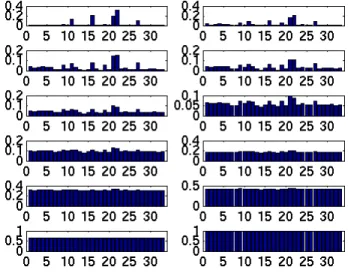
Figure 1. Kernel weights learnt on the training set with variouspvalues. “dog” class. From left to right, top to bottom:p={1,1 + 2−6,1 +
2−5,1+2−4,1+2−3,1+2−2,1+2−1,2,3,4,8,106}.
Table 2. MK-FDAs with original kernels
`1MK-FDA `2MK-FDA `∞MK-FDA `pMK-FDA
MAP 54.85 54.79 54.64 55.61
{1,1 + 2−6,1 + 2−5,1 + 2−4,1 + 2−3,1 + 2−2,1 +
2−1,2,3,4,8,106}, and then apply the learnt optimalpto test set. We compare this`p MK-FDA scheme with fixed-norm MK-FDA, where the regularisation fixed-norm is fixed to `1,`2, and`∞.
Shown in Fig. 1 are the kernel weights learnt on the training set with various regularisation norms for the “dog” class. This figure confirms that the normpcontrols the spar-sity of the learnt weights: the smaller the value, the more sparse the weights. Whenp= 106(practically infinity), the kernels weights become ones, i.e.,`∞MK-FDA is
equiva-lent to single kernel FDA with uniformly weighted sum of the base kernels.
In Table 2, we show MAPs of the four MK-FDA meth-ods. By tuning the regularisation normpusing the valida-tion set, the intrinsic sparsity of the kernel set can be learnt. As a result,`pMK-FDA outperforms its fixed norm coun-terparts.
4.3
Results with denoised kernels
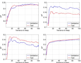
In this section we show the effect of feature space de-noising using kernel PCA. We again use the “dog” class as an example. Fig. 2 plots the APs obtained with single kernel FDA on the validation set and test set when keeping various
Figure 2. Feature space denoising with ker-nel PCA. “dog” class. Top left: kerker-nel 21. Top right: kernel 26. Bottom left: kernel 30. Bot-tom right: sum of all 33 base kernels.
Table 3. MK-FDAs with denoised kernels
`1MK-FDA `2MK-FDA `∞MK-FDA `pMK-FDA
MAP 54.26 56.06 55.82 56.17
amount of variance in kernel PCA. The first three subplots are with three base kernels, and the bottom left one is with the sum of all 33 base kernels.
Fig. 2 top and bottom left show that the performance curve on the validation set is a good indicator of the amount of noise in the feature space. In other words, one can de-termine how much variance to retain, or equivalently how much noise to remove, based on this curve. The optimal amount of variance to keep is kernel dependent (∼20%for kernel 26 and kernel 30,∼80%for kernel 21), but feature space denoising consistently boosts the performance on the test set compared to using the whole feature space without denoising.
Another interesting observation is that when applying feature space denoising to the sum of all 33 base kernels, we do not obtain any improvement (Fig. 2, bottom right). In this case, The best performance on both validation and test sets are achieved when all dimensions of the feature space are used. The MAP of this “summing + denoising” strategy is 54.37: compared to the “summing only” strat-egy (`∞MK-FDA in Table 2), the performance even drops
slightly.
Considering these observations, a more reasonable strat-egy would be to first denoise each base kernel, and then apply`pMK-FDA. The results of such a strategy are shown
Figure 3. Spearman’s coefficient between the learnt kernel weights and percentage of vari-ance to keep.
in Table 3. Note that the`∞MK-FDA in the table is
sim-ply a “denoising + summing” scheme. Its advantage over the “summing + denoising” scheme is evident (55.82 vs. 54.37).
With the denoised kernels, the `p MK-FDA again out-performs the fixed-norm versions. However, the margin be-tween it and its competitors is smaller this time. For exam-ple, it outperforms the`2version only by 0.11. This seems to suggest that much of the benefit of MKL comes from its tendency to assign small weights to noisy kernels and vice versa. In order to test this hypothesis, we rank the 33 base kernels according to the kernel weights learnt with the opti-malpvalue. We then rank the base kernels again according to the amount of variance kept by the feature space denois-ing process. If our hypothesis is correct, the two rankdenois-ings should show some consistency.
We use Spearman’s rank correlation coefficient [15] to measure the similarity between the two rankings. A coeffi-cient of +1 indicates identical rankings, while a coefficoeffi-cient of -1 means the two rankings are reversed of each other. The Spearman’s coefficients for the 20 object classes are shown in Fig. 3. Out of 20, positive coefficients are ob-served on 16 object classes, and negative coefficients are observed only on 3 classes. On the “sheep” class the opti-mal kernel weights learnt are uniform, for which case the Spearman’s coefficient is not defined. The mean of the 19 Spearman’s coefficients is 0.1917, which indicates there is indeed some correlation between the kernel weights learnt in MKL and the noise level in the base kernels.
In the experiments, the stopping thresholdin`p MK-FDA is set to10−4, andλis also set to10−4. The kernels used in the paper and a Matlab implementation of`p
MK-FDA are available online3.
5
Conclusions
In this paper, we have reviewed an MKL technique, namely,`pregularised MK-FDA, and have investigated the effect of feature space denoising by means of kernel PCA. Experiments show that with both the original base kernels or denoised base kernels, by learning their intrinsic spar-sity using a validation set, the `p MK-FDA we recently proposed outperforms its fixed-norm counterparts. Exper-iments also show that feature space denoising boosts the performance of both single kernel FDA and the `p MK-FDA. This observation, together with the one that there is in general a positive correlation between the learnt kernel weights in`pMK-FDA and the amount of variance kept by feature space denoising, seems to suggest that MKL should be performed on a per dimension basis instead of per kernel basis. However, this is not possible with MKL techniques that learn linear combinations of base kernels. An MKL objective function which can take care of the feature space denoising automatically, and which can learn a truly opti-mal (non-linear) combination of the base kernels, is yet to be found.
Acknowledgement
This work has been supported by EPSRC ACASVA Grant EP/F069421/1.
References
[1] F. Bach and G. Lanckriet. Multiple kernel learning, conic duality, and the smo algorithm. InICML, 2004.
[2] G. Baudat and F. Anouar. Generalized discriminant analy-sis using a kernel approach.Neural Computation, 12:2385– 2404, 2000.
[3] M. Everingham, L. Van Gool, C. K. I. Williams, J. Winn, and A. Zisserman. The PASCAL Visual Object Classes Challenge 2007 (VOC2007) Results. http://www.pascal-network.org/challenges/VOC/voc2007/workshop/index.html. [4] R. Hettich and K. Kortanek. Semi-infinite
program-ming: Theory, methods, and applications. SIAM Review, 35(3):380–429, 1993.
[5] S. Ji, L. Sun, R. Jin, and J. Ye. Multilabel multiple kernel learning. InNIPS, 2008.
[6] S. Kim, A. Magnani, and S. Boyd. Optimal kernel selection in kernel fisher discriminant analysis. InICML, 2006. [7] M. Kloft, U. Brefeld, S. Sonnenburg, and A. Zien. Efficient
and accurate lp-norm mkl. InNIPS, 2009.
3http://www.featurespace.org
[8] G. Lanckriet, N. Cristianini, P. Bartlett, L. E. Ghaoui, and M. Jordan. Learning the kernel matrix with semidefinite pro-gramming.JMLR, 5:27–72, 2004.
[9] S. Mika. Kernel fisher discriminants. PhD Thesis, University of Technology, Berlin, Germany, 2002.
[10] A. Rakotomamonjy, F. Bach, Y. Grandvalet, and S. Canu. Simplemkl.JMLR, 9:2491–2521, 2008.
[11] B. Scholkopf and A. Smola. Learning with Kernels. MIT Press, 2002.
[12] B. Scholkopf, A. Smola, and K. Muller. Kernel principal component analysis. Advances in Kernel Methods: Support Vector Learning, pages 327–352, 1999.
[13] J. Shawe-Taylor and N. Cristianini.Kernel Methods for Pat-tern Analysis. Cambridge University Press, 2004.
[14] S. Sonnenburg, G. Ratsch, C. Schafer, and B. Scholkopf. Large scale multiple kernel learning. JMLR, 7:1531–1565, 2006.
[15] C. Spearman. The proof and measurement of association be-tween two things.Ameriman Journal of Psychology, 15:72– 101, 1904.
[16] V. Vapnik. The Nature of Statistical Learning Theory. Springer-Verlag, 1999.
[17] F. Yan, J. Kittler, K. Mikolajczyk, and A. Tahir. Non-sparse multiple kernel learning for fisher discriminant analysis. In
International Conference on Data Mining, 2009.
[18] F. Yan, K. Mikolajczyk, M. Barnard, H. Cai, and J. Kittler. Lp norm multiple kernel fisher discriminant analysis for ob-ject and image categorisation. InCVPR, 2010.
[19] J. Ye, S. Ji, and J. Chen. Multi-class discriminant kernel learning via convex programming.JMLR, 9:719–758, 2008. [20] A. Zien and C. Ong. Multiclass multiple kernel learning. In