Anomaly Detection in Dynamic Networks

(1)

Anomaly Detection in Dynamic Networks

A thesis presented for the degree of

Doctor of Philosophy of Imperial College London and the

Diploma of Imperial College by

Melissa Turcotte

Department of Mathematics Imperial College

180 Queen’s Gate, London, SW7 2AZ

(2)

2

I certify that this thesis, and the research to which it refers, are the product of my own work, and that any ideas or quotations from the work of other people, published or otherwise, are fully acknowledged in accordance with the standard referencing practices of the discipline.

(3)

3

Copyright

The copyright of this thesis rests with the author and is made available under a Creative Com-mons Attribution Non-Commercial No Derivatives licence. Researchers are free to copy, dis-tribute or transmit the thesis on the condition that they atdis-tribute it, that they do not use it for commercial purposes and that they do not alter, transform or build upon it. For any reuse or redistribution, researchers must make clear to others the licence terms of this work.

(4)

4

Acknowledgements

First I would like to thank my supervisor, Nick Heard, for his encouragement and immense support throughout my PhD. From the start, Nick has made research exciting and engaging and I consider myself extremely fortunate to have been supervised by him. Throughout my PhD Nick went out of his way to create fantastic opportunities for furthering my career and for this I am extremely grateful. He also deserves extra credit for his infinite patience in dealing with me, I imagine it was difficult at times.

I would also like to acknowledge all the people whom I worked with and got to know at ACS-PO at Los Alamos National Laboratory, without their expertise and support the chapter on computer network security would not have been possible. In particular, I would like to thank Joshua Neil, who supervised me during my time at Los Alamos and introduced me to the challenges of cyber-security. His genuine enthusiasm for this particular problem makes him a pleasure to work with.

I would like to recognise the support from EPSRC and the Institute for Security Science and Technology at Imperial College London for funding this research.

Finally, Niall Adams, Patrick Rubin-Delanchy and Ed Cohen deserve a mention for the many stimulating discussions throughout my time at Imperial and generally creating a very pleasant work environment.

(5)

5

Abstract

Anomaly detection in dynamic communication networks has many important security applica-tions. These networks can be extremely large and so detecting any changes in their structure can be computationally challenging; hence, computationally fast, parallelisable methods for moni-toring the network are paramount. For this reason the methods presented here use independent node and edge based models to detect locally anomalous substructures within communication networks. As a first stage, the aim is to detect changes in the data streams arising from node or edge communications. Throughout the thesis simple, conjugate Bayesian models for counting processes are used to model these data streams. A second stage of analysis can then be per-formed on a much reduced subset of the network comprising nodes and edges which have been identified as potentially anomalous in the first stage.

The first method assumes communications in a network arise from an inhomogeneous Pois-son process with piecewise constant intensity. Anomaly detection is then treated as a change-point problem on the intensities. The changechange-point model is extended to incorporate seasonal behaviour inherent in communication networks. This seasonal behaviour is also viewed as a changepoint problem acting on a piecewise constant Poisson process. In a static time frame, inference is made on this extended model via a Gibbs sampling strategy. In a sequential time frame, where the data arrive as a stream, a novel, fast Sequential Monte Carlo (SMC) algorithm is introduced to sample from the sequence of posterior distributions of the changepoints over time.

A second method is considered for monitoring communications in a large scale computer network. The usage patterns in these types of networks are very bursty in nature and don’t fit a

(6)

6

Poisson process model. For tractable inference, discrete time models are considered, where the data are aggregated into discrete time periods and probability models are fitted to the commu-nication counts. In a sequential analysis, anomalous behaviour is then identified from outlying behaviour with respect to the fitted predictive probability models. Seasonality is again incor-porated into the model and is treated as a changepoint model on the transition probabilities of a discrete time Markov process. Second stage analytics are then developed which combine anomalous edges to identify anomalous substructures in the network.

(7)

7

List of Figures

1.1 VAST data event times organised by individual . . . 20

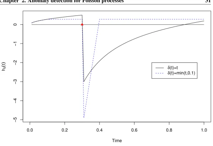
2.1 hδ(t)given a changepoint at 0.3 withν = 1. . . 31

3.1 Histogram of call start times for the VAST data set . . . 36

3.2 Posterior changepoint distributions . . . 37

3.3 Number of anomalous individuals in the VAST data set . . . 38

3.4 Spectral cluster plot of the anomalous individuals in the VAST data set . . . 40

3.5 Number of anomalous individuals in the VAST data set using the approximate model . . . 42

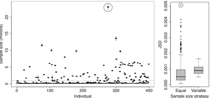
3.6 Box plot of the allocated sample sizes and the Jensen-Shannon divergence . . . 49

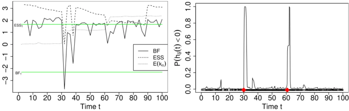
4.1 Left: ESS, BF and the online estimate of the expected number of changepoints. Right: Online estimate ofP_π_(h_min(t,2)_(t)_<₀₎_{. . . .} ₆₇

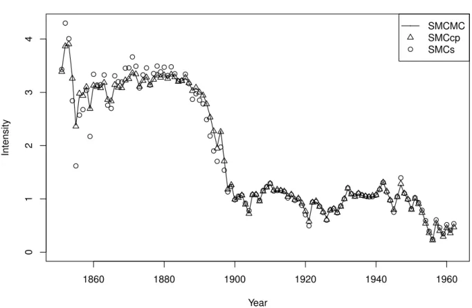
4.2 Online estimated intensity function for the coal-mining disaster data . . . 74

4.3 Effective sample size . . . 74

4.4 Posterior changepoint distributions . . . 75

4.5 Number of anomalous individuals in the VAST data . . . 77

4.6 Online estimate ofP_π_(h_t_(t)_<₀₎_{for the individual with ID}₃₉₂_{. . . .} ₇₈

4.7 Box plot of the sample sizes allocated to each individual on each update interval 79 4.8 Allocated sample sizes for each update interval . . . 79

5.1 An example of a traversal attack . . . 83

5.2 Number of active nodes and edges in the LANL data . . . 84

5.3 Activity status of an edge in the LANL computer network . . . 85

5.4 Maximum count versus the median count for the observed counts in the training period for a random sample of3,000edges. . . 85

5.5 Activity status of a node in the LANL computer network . . . 90

5.6 The empirical count distribution with the corresponding fitted Negative Bino-mial and Poisson distributions . . . 94

5.7 Empirical distribution of the autocorrelation function lag 1. . . 95

5.8 Anomaly scores for components of the anomaly graphs . . . 102

5.9 Heat map of the first detected anomalous component . . . 103

5.10 Heat map of component containing anomalous hosts . . . 104

5.11 Indegree of the two core servers in the LANL computer network . . . 105

(10)

10

List of Tables

4.1 Results from the SMC and SMCMC algorithms for the 100 simulations. For

the first three rival methods the summary statistics are the averages across all

(11)

11

List of Algorithms

1 Gibbs Sampler . . . 35

2 Approximate Gibbs sampler . . . 41

3 Sample allocation for rival samplers . . . 48

4 Increasing particle set from N to M . . . 63

(12)

12

Chapter 1 Introduction

Networks are representational forms for systems in nature, society and technology. Kolaczyk (2000) gives a good overview of networks and example contexts in which they arise. Dynamic networks are generally regarded as networks that evolve over time. Networks are often repre-sented by graphs with a finite set of nodes or vertices and edges defining the pairwise relations between them. Relations may not continuously exist between two nodes and often edges rep-resent sequences of instantaneous communications. Hence the information about a dynamic

network is stored in a time series of graphs{Gt}, whereGtconsists of a set of nodes and edges

that exist at timet. In practice the node set could also be changing over time but for the purposes

of this thesis it is assumed that there is a fixed number of entities in the network and the edges between them evolve over time.

Anomaly detection in dynamic networks is the continuous monitoring of these time evolv-ing graphs for unusual events or trends. The precise definition of an anomaly depends on the application of interest but could be characterised by sudden changes in connectivity between nodes in a network, new ties forming between seemingly unrelated nodes or general irregular changes within the substructure of the graph. Generally anomaly detection systems aim to build a model based on normal graph characteristics that are observed from the network over time and then search for outlying behaviour with respect to the model, indicating the presence of unusual or possibly malicious behaviour in the network. The survey by Chandola et al. (2009) provides

(13)

Chapter 1. Introduction 13

a comprehensive overview of various anomaly detection techniques and their applications. An-other large area of research is signature-based anomaly detection where signatures based on previous attacks are used to search for current attack behaviour, (Axelsson, 2000; Cahill et al., 2004). Non signature-based anomaly detection differs in that any type of deviations from the normal state of the network are sought and has a clear advantage in that new types of threats can be identified.

The application for the work in this thesis is anomaly detection in communication networks; in particular, in the context of monitoring for security purposes. There are many security con-texts in which monitoring a large dynamic network for suspicious or fraudulent behaviour is important and two motivating network examples are considered: telecommunication networks and computer networks. Monitoring telecommunication networks for fraudulent behaviour is a well established problem and another context that has important significance to government agencies, is the online surveillance of these networks to uncover terrorist cells. Computer net-works are of rapidly growing importance. With advances in networking technology and the reliance on these technologies within government and commercial enterprises, the threat from cyber-attacks has drastically increased and keeping computer networks secure is now critically important.

For most of the thesis anomaly detection is viewed as a changepoint problem and novel algorithms are developed for performing changepoint analysis on a collection of stochastic pro-cesses in both the static and continuous time frames. The main contribution of the thesis is a novel sequential Monte Carlo (SMC) algorithm for sequential changepoint detection that is computationally fast and obtains the most efficiency when applied across a large number of data streams.

More generally, a dynamic sample size allocation strategy is presented for making optimal use of a fixed computational resource when analysing multiple data streams. Sampling effort is allocated sequentially to the posterior distributions relating to the data streams according to the estimated relative complexities of those distributions. This problem has not previously been considered in the literature.

(14)

1.1 Anomaly detection approach 14

Finally, seasonality in behaviour, which is inherent in user driven communication networks, is also treated as a changepoint problem and this is also novel with respect to the current lit-erature. The final chapter of the thesis is concerned with using statistical models for anomaly detection in computer networks. Statistical modelling for cyber security is a relatively new area of research in statistics, and an anomaly detection system is developed for a specific application of cyber security: detecting an intruder in a internal computer network (Neil et al., 2013a).

1.1 Anomaly detection approach

Communication networks such as telecommunication or computer networks are typically very large with thousands or millions of edges at any one time. To enable deployment on large graphs any anomaly detection schemes have to be computationally fast, scalable and ideally parallelisable.

One method of anomaly detection in networks is concerned with finding anomalous structures of the network. Spectral graph techniques are commonly used to find unusual sub-graphs such as small cliques or nodes with unusual neighbourhoods (von Luxburg, 2007; Skil-licorn, 2007; Id´e and Kashima, 2004). Scan statistics have also been used in detecting local anomalies in networks (Priebe et al., 2005), where a local statistic for some graph invariant is calculated over sliding windows. The maximum across the graph of the locality statistic is de-fined as the scan statistic and compared against some null hypothesis of normal behaviour. In Park et al. (2013) this is extended so that a fusion of graph invariants are considered. For social networks analysis, methods have been developed that infer information about links and nodes over time using information from an existing set of attributes for the network graph such as node labels (Cortes et al., 2003; Rhodes and Keefe, 2007). All of these approaches either place an implicit specification of the type of anomaly sought or have a high computational cost when applying them to larger networks. For a more general overview of various techniques related to anomaly detection see Chandola et al. (2009)

(15)

independent or conditionally independent entities that have an associated counting process de-scribing the communications process of that node or edge. For telecommunication networks this process could represent the timings of phone calls, or in computer networks the connec-tion times between pairs of IP addresses. Heard et al. (2010) suggests that if a network has fundamentally changed in some significant way then in most contexts this indicates that some entities are communicating more or less frequently or there are new links between entities. A two-stage approach, as presented in Heard et al. (2010), will be used for the work in this thesis. First, potentially anomalous nodes are identified by deviations from their usual connectivity by treating either the pairwise communications or the directed or undirected communications for single entities as independent processes. Initially taking this broad view allows a fast sweep of the whole network to identify good anomalous targets to zoom in on. The second stage is then to construct a subgraph around these anomalous nodes, this will give a much reduced sub-network for which standard graph analysis tools can be more feasibly deployed to examine the more subtle network structure.

In this thesis, anomaly detection in networks is viewed from both continuous and discrete time perspectives. Simple conjugate Bayesian models are used for both perspectives allowing for fast tractable inference, which is imperative for the large networks of interest.

For the first motivating problem, which is anomaly detection in telecommunication net-works, the event times emanating from each edge or node in the graph are treated as continuous time counting processes that are monitored for changes over time. Frost and Melamed (1994) gives an overview of commonly used models for telecommunications traffic. Inhomogeneous Poisson processes with piecewise constant intensities, where the jumps in the intensity corre-spond to changepoints or anomalies, provide a flexible, computationally tractable framework.

The main focus of this thesis is developing algorithms for changepoint detection on the col-lection of stochastic processes emanating from each node or edge. In particular a new sequential Monte Carlo algorithm is presented for fast sequential changepoint detection. Although the al-gorithm is designed primarily for online changepoint detection for continuous time processes, it can also be used for discrete time processes.

(16)

1.2 Bayesian changepoint modelling 16

For the second motivating example, detecting an intruder on a computer network, discrete time models are used where the time domain is aggregated into intervals and statistical sum-maries of activity are collected in each interval, such as the number of connections made along an edge, to form a discrete time stochastic process. For computer network data the continuous time models used for the telecommunication networks would not be appropriate for the “bursty” behaviour that is observed.

A probability model is sequentially fitted to the discrete time process using the data ob-served so far. Independent hierarchical models are used to model each node’s activity status and then conditionally on that node’s status, edges are modelled conditionally independent of one another. Anomalies are then defined to be observations with low predictive probability ac-cording to the fitted model. This is an extension of the work in Heard et al. (2010), which was applied to a much simpler telecommunication network problem.

Seasonality inherent in these user driven networks adds to the challenge of monitoring these processes. For both the continuous and discrete time perspectives seasonality is also viewed as a changepoint problem. In continuous time the changepoint model for the intensity of an inhomogeneous Poisson process is extended to include seasonal changepoints and for the dis-crete time models the seasonal changepoints act on the transition probabilities of a disdis-crete time Markov chain modelling the on/off activity status of nodes in the network.

As changepoint models underpin most of the methodology presented in this thesis, the fol-lowing section gives a brief introduction to the Bayesian changepoint model.

1.2 Bayesian changepoint modelling

Changepoint models are widely used for many data analysis problems where the data generat-ing process begenerat-ing observed undergoes characteristic changes over time. A possibly unknown number of changepoints split up the data into disjoint segments, where the data are assumed to arise from a single generative model within each segment but different models across seg-ments. Changepoint detection is concerned with finding the location of these changes, and in a

(17)

sequential setting, detecting the change soon after it has occurred. Changepoint models can broadly be split up into two categories:

1. The data across segments follow unrelated probability distributions; in a non-parametric setting these would be considered unknown, or

2. The data follow a probability distribution of the same functional form but the underlying parameters of the model change between segments.

This thesis and all the references to changepoint models within are concerned with inference on data that is assumed to fall under the latter category.

Models that have been considered in the literature include piecewise constant intensity Pois-son processes (Green, 1995; Carlin et al., 1992; Fearnhead, 2006; Hawkins, 2001; Del Moral et al., 2006); changing linear regression (Carlin et al., 1992; Stephens, 1994; Barry and Harti-gan, 1993; Fearnhead, 2006; Hinkley, 1970; Breiman et al., 1984; Hawkins, 2001) and Markov models with time-varying transition matrices (Carlin et al., 1992). These models are used in many applications such as finance, engineering and quality control.

Let{y(t) : 0 ≤ t ≤ T}be a stochastic process on[0, T], which will be referred to as the

data. For notational brevity, the values taken by the process over any subsetB ⊆ [0, T]will be

denoted asy(B); soy(B) ={(t, y(t)) :t∈B}.

The changepoint model assumes that an unknown number of changepoints split up the data into disjoint segments where the data in each of the segments are typically independent of one

another. Here it is further assumed that the distribution ofy(t)varies between segments only

through changes in a generic parameter vectorθ ∈Θ.

Let k be the number of changepoints over [0, T]. If k = 0 let τ1:k = ∅, else if k > 0

letτ1:k = (τ1, . . . , τk)represent the ordered locations of these changepoints, so thatτ1:k ∈ Tk

where

T_k ₌_{_τ_1:k _{: 0}_{< τ}₁ _{< . . . < τ}_k _{< T}_}_.

The changepoints,τ1:k split up the data intok+ 1independent segments. For simple notation

(18)

1.2 Bayesian changepoint modelling 18

observed process data in each segmenty((τi, τi+1])fori= 0, . . . , k.

Given the vectors of changepoints and parameters, the likelihood of the data over the interval

[0, T]can then be expressed as

L(y([0, T])|τ1:k, k, θ0:k) =

k

Y

i=0

L(y((τi, τi+1])|θi),

whereL(·|θi)is a generic likelihood function for the data generating process given fixed

pa-rametersθi.

Given a prior distribution for the parameters and the changepoints, denotedp(τ1:k, k, θ0:k),

the posterior distribution of interest over the interval[0, T]given the observed process data is

π(τ1:k, k, θ0:k|y([0, T])) =

γ(τ1:k, k, θ0:k, y([0, T]))

Z , (1.1)

where

γ(τ1:k, k, θ0:k, y([0, T])) =L(y([0, T])|τ1:k, k, θ0:k)p(τ1:k, k, θ0:k) (1.2)

is assumed to be known pointwise andZ, which is the corresponding normalising constant of

π, may not be known.

The priorp(τ1:k, k, θ0:k)and the posteriorπ(τ1:k, k, θ0:k|y([0, T]))both have support on the

disjoint union EΘ= ∞ [ k=0 {k} ×Θk+1×T_k_.

The prior on the parameters and the changepoints is typically constructed as

p(τ1:k, k, θ0:k) =p(τ1:k, k)p(θ0:k|τ1:k, k),

where under the assumption of independence of the parameters between segments,

p(θ0:k|τ1:k, k) = k

Y

i=0

(19)

If the model parametersθ0:kcan be integrated out from (1.2), as is the case whenp(θi)is chosen

to be the conjugate prior for the likelihood function for the data, then the marginal likelihood function of the data given the changepoints

L(y([0, T])|τ1:k, k) = k Y i=0 Z L(y((τi, τi+1])|θi)p(θi) dθi (1.3)

can be obtained. The posterior distribution of the changepoints given the data is then

π(τ1:k, k|y([0, T])) = γ(τ1:k, k, y[0, T])) Z , (1.4) with support E = ∞ [ k=0 {k} ×T_k_.

For simplification of notation throughout the rest of the thesis, where appropriate, when

refer-ring to the posterior distribution of (1.4) the dependency onkand the data will be suppressed,

so that γ(τ1:k) = γ(τ1:k, k, y([0, T])) and π(τ1:k) = π(τ1:k, k|y([0, T])) over some specified

interval[0, T].

1.3 Data sets

Two network data sets are used for demonstrations of the methods developed in this thesis. A description of the first data set, which is used in Chapters 2, 3 and 4 for the continuous time models, is given below. The second data set, which is from Los Alamos National Laboratory’s large internal computer network, is described in Section 5.1 in Chapter 5.