University of Toronto
Department of Economics
March 30, 2007
By John M Maheu and Stephen Gordon
Learning, Forecasting and Structural Breaks
Learning, Forecasting and Structural Breaks
∗
John M. Maheu
†Stephen Gordon
‡First draft July 2004
This draft March 2007
Abstract
We provide a general methodology for forecasting in the presence of structural breaks induced by unpredictable changes to model parameters. Bayesian methods of learning and model comparison are used to derive a predictive density that takes into account the possibility that a break will occur before the next observation. Estimates for the posterior distribution of the most recent break are generated as a by-product of our procedure. We discuss the importance of using priors that accurately reflect the econometrician’s opinions as to what constitutes a plausible forecast. Several applications to macroeconomic time-series data demonstrate the usefulness of our procedure.
Keywords: Bayesian Model Averaging, Markov Chain Monte Carlo, Real GDP Growth, Phillip’s Curve
∗Both authors are grateful for helpful comments from M. Hashem Pesaran, Herman K. van Dijk, two
anonymous referees, James MacKinnon, Tom McCurdy, Simon van Norden, and seminar participants from the Midwest Econometrics Group, the Canadian Economics Association Annual Meetings and the University of Toronto. Financial support from the Social Sciences and Humanities Research Council of Canada is gratefully acknowledged.
†Corresponding author: Department of Economics, 100 St. George St., University of Toronto,
Toronto, Canada, M5S 3G3, phone 416-978-1495, fax 416-978-6713, [email protected].
‡D´epartement d’´economique and CIRP´EE, Universit´e Laval, Quebec City, Quebec, G1K 7P4,
1
Introduction
There is a considerable body of evidence that documents the instability of many im-portant relationships among economic variables. Popular examples include the Phillip’s curve, U.S. interest rates and the demand for money.1 An important challenge facing
modern economics is the modeling of these unstable relationships. For econometricians, the difficulties involve estimation, inference and forecasting in the presence of possible structural instability.
Classical approaches to the identification of break points are based on asymptotic theory - see, for example, Ghysels and Hall (1990), Hansen (1992), Andrews (1993), Dufour et al. (1994), Ghysels et al. (1997), and Andrews (2003) - are based on frameworks in which both the pre-break and post-break data samples go to infinity.2 Moreover,
tests for multiple breaks such as those proposed by Andrews et al. (1996), and Bai and Perron (1998) are also based on similar assumptions. In applications that make use of available finite data sets, the empirical relevance of such an assumption may be suspect. Furthermore, the statistical properties of a forecasting model based on classical breakpoint tests are far from clear, since such a model would be based on a pre-test estimator.
In contrast, Bayesian approaches to the problem are theoretically simple, are based on finite-sample inference, and typically take the form of a simple model comparison exercise. Examples include Incl´an (1994), Chib (1998), Wang and Zivot (2000), Kim et al. (2004), and Giordani and Kohn (2006) which employ Markov Chain Monte Carlo sampling methods to make posterior inferences regarding the timing of break points in a given sample.
A feature that is common to both strands of the existing literature is the focus on the
ex postidentification of structural breaks that may have occurred in the past. While this question is of course important in itself, economists are more likely to be interested in making forecasts when the the data generating process is unstable. This is the question that we address here. More precisely, we focus on the question of how to make optimal use of past data to forecast out-of-sample while taking into account the possibility that breaks have occurred in the past, as well as the possibility that they may occur in the future.
Koop and Potter (2004), and Pesaran et al. (2006) consider forecasting in the presence of breaks. They extend the work of Chib (1998) in which breaks are assumed to be governed by a first-order Markov chain. Using ideas in Carlin et al. (1992), Pesaran et al. (2006) assume that break parameters are drawn from a common meta distribution. In a similar spirit, nonlinear models such as regime switching models (Hamilton (1989)), and time-varying parameter models (Cogley and Sargent (2002), Kim and
Nel-1Stock and Watson (1996) suggest that the laws of motion governing the evolution of many important macroeconomic time series appear to be unstable.
2The theory of Dufour et al. (1994) and Andrews (2003) only requires that the structurally stable portion of the data goes to infinity.
son (1999), Koop and Potter (2001), McCulloch and Tsay (1993) , Nicholls and Pagan (1985)) allow for changes in the form of the conditional density of the data, but these are assumed to evolve according to a fixed law of motion. Parameters change over time, but in a predictable way.
In contrast, we define a structural break as an unpredictable event in which the relationship among the variables in a model changes, and this change cannot be predicted in any sense from past data. By this definition we would classify many models, such as time varying parameter specifications, as nonlinear models since they assume a structure for changes in parameters and learn about future breaks from past data.3 Therefore, we
are interested in structural breaks that cannot be modeled and predicted in the usual sense based on mathematical models and historical data.
The distinguishing feature of the methods developed in this study is the potential role of non-sample information that becomes available to the analyst after the first ob-servation. In the applications of Bayesian methods mentioned above, it is assumed that all non-sample information can be incorporated in a prior that is specified before observ-ing the data; these beliefs are then continually revised as new data are observed. But in many interesting real-world forecasting problems, analysts may receive non-sample information about a possible structural break after the first observation, but before the actual breakpoint. As an example, consider the Phillips curve prior to the 1970s, which many economists and policy makers believed was a stable relationship between inflation and unemployment. In the late 1960s Milton Friedman (Friedman (1968)) predicted the subsequent instability of the Phillips curve that was observed in later years.4 What does
the analyst do when non-sample information, such as new economic theory, suggests that a structural break in an empirical model may occur in the future?
We present a general methodology for economic decision making based on a model subject to discrete structural breaks. Each structural break is assumed to be a unique event that has a different impact on model parameters. In this sense past breaks are not informative about future breaks. For example, we find unrelated events such as the Korean war, the oil shocks in the 1970s, and changes in monetary policy are associated with structural breaks in our results. On the other hand, if we assume a specific break process, like an iid Bernoulli distribution, we show how the probability of a break can be estimated from sample data.
Our analysis uses adaptive learning via Bayes’ rule in order to make optimal use of past data to make forecasts. We allow for breaks to occur at every observation and when a break occurs the new parameters are assumed to be unrelated to the past.5
This assumption is consistent with our definition of a structural break and it leads to a simplification in computation.
The use of data observed before a structural break could result in a bias in estimates
3Alternatively, it may be clearer to say that we are concerned withunpredictable structural breaks and not nonlinear dynamics.
4Phelps (1967) also predicted problems for the Phillips curve. 5We relax this assumption in the Phillips curve example.
and forecast; a rolling window estimator that uses a portion of the available data is a possible solution. However, this may not be optimal, as some combination of the data that follows a perceived break, and the data that preceded it, may be a better solution. Our approach optimally combines models based on longer histories of data which may contain breaks but provide more precise forecasts, with models based on shorter histories of data which are less influenced by past breaks but have less precise forecasts. Although there is a potential tradeoff between the accuracy of a forecast and its precision; our results suggest that the predictive standard deviations generated by our approach are generally similar to those of other models.
Our structural break model is constructed from a series of submodels. Each submodel has an identical parameterization but the parameter is estimated from a different history of data. Each submodel identifies a unique break point, and learning begins from the prior as new data arrives after the break point. Submodels are differentiated by when they start and the data they use. New submodels are continually introduced through time to allow for multiple structural breaks, and for a potential break out-of-sample.
Since structural breaks can never be identified with certainty, Bayesian model aver-aging provides a predictive distribution, which accounts for past and future structural breaks, by integrating over each of the possible submodels weighted by their probabili-ties. Therefore new submodels, which are based on recent shorter histories of data, only receive significant weights once their predictive performance warrants it. As a byprod-uct of estimation, our procedure provides estimates for the posterior probability of the most recent break in the sample, as well as the posterior distribution for the number of observations that would be useful in making out-of-sample forecasts.
Our approach is closely related to Pesaran and Timmermann (2007) which inves-tigates the selection of an estimation window in the presence of breaks. They show that it can be optimal to use pre-break data to improve the trade-off between bias and forecast error variance. Like Pesaran and Timmermann (2002) we focus on the most recent break in the past.6 In our context, each of the submodels is based on a different
history of data, but we average over each of the submodel predictions using the model probabilities. The model probabilities are based on past past predictive content of each of the submodels and determines the tradeoff between bias and forecast error variance. The main differences of our approach to forecasting in the presence of breaks with Koop and Potter (2004), and Pesaran et al. (2006) is that they use a hidden Markov chain embedded in the model to capture the effect of breaks. In contrast we decouple the submodel parameter estimation from estimation of the structural break process. This simplifies the computational burden. This means there are two steps to estimation and forecasting.7 For example, in one example we assume the probability of a break is a
constant and use past data to estimate it. The submodels and their predictive likelihoods
6Pesaran and Timmermann (2002) use a reversed order CUSUM test to identify the most recent break. This is closely related to our concept ofmean useful observations discussed in Section 2.
7When the probability of the break is set subjectively using non-sample information the second step in estimation is unnecessary, however, submodel probabilities must be computed.
are estimated independent of the break process (except for the history of data used). Estimation of the break probability only uses the submodel predictive likelihoods, which makes this second step of estimation very easy. This simplification of estimation of the break process carries over to other more complicated submodel specifications as long as a submodel predictive likelihood can be efficiently computed. In addition, our model averaging approach makes it easy to allow for recursive out-of-sample forecasts in the presence of an increasing number of structural breaks through time.
Like time-varying parameter models, such as Primiceri (2005), we allow for breaks in every submodel parameter. We also allow for a break every period but we do not assume it, and in general we expect infrequent breaks to occur. Thus our focus is on abrupt parameter change and not gradual change as in Primiceri (2005). Koop and Potter (2004) provide a method that allows for these two extremes as well as something in between. On the other hand, it is difficult to allow for breaks in only a subset of submodel parameters: unless the posteriors for the stable and unstable parameters are independent, revisions in the beliefs about the unstable parameters will induce revisions in the posterior for stable parameters. We discuss methods to incorporate the belief that only some parameters are unstable by calibrating new submodel priors with past data. Finally, our target is the predictive density given our assumptions about breaks. Inference on the most recent structural break is only a byproduct, and this is meant to occur in real time. As such, an historical in-sample analysis of the number of breaks may be better achieved with the Chib change-point model.
Several applications of the theory to simulated, and macroeconomic time-series data are discussed. In comparison to a model that assumes no breaks, we find the method produces very good out-of-sample forecasts, accurately identifies breaks, and performs well when the data do not contain breaks. In particular, the examples demonstrate that a break can result in a large jump in the predictive variance, which quickly reduces as we learn about the new parameters. However, models that ignore breaks, may have a long-term rise in the predictive variance. As a result, our method can be expected to produce more realistic moments, and quantiles of the predictive density.
We consider predictions of real U.S. GDP and document the reduction in variability discussed in Stock and Watson (2002) among others. Rather than a one time break in volatility, our results point to a gradual reduction in volatility over time with evidence of 3 separate regimes. The model is particularly useful in forecasting the probability of positive growth. We compare our forecasting approach to the in-sample break-point model of Chib (1998) and show that we produce similar results. An important difference is that our approach is designed for prediction, and as such integrates over all past structural breaks in producing posterior inference for parameters or an out-of-sample prediction.
A second application considers a forecasting model of inflation motivated from a Phillips curve relationship. There are several breaks in this model and a considerable amount of parameter instability. By accounting for these breaks in the process, our approach delivers improved forecasting precision for inflation. The identified breaks,
which are not exclusively associated with oil shocks, indicate that the Phillips curve we use is far from stable. However, the structural break model optimally extracts any predictive value from this unstable relationship. The best performing model is a struc-tural break specification in which the prior on the variance parameter σ2 of each new
submodel is calibrated to the last period’s posterior mean of σ2. This model produces
the best marginal likelihood values and competitive forecasts as compared to several other specifications.
This paper is organized as follows. Section 2 provides a more detailed explanation of the approach, as well as a description of techniques that can be used to implement the procedure. Our main approach assumes that breaks are set subjectively by the econometrician, however, we show how the model can be extended to estimate the break process from past data. Section 3 applies these methods to simulated data, growth rates in US GDP and to a Phillips curve model of inflation. Section 4 discusses results and extensions.
2
Learning about structural breaks
In this section we provide details of the structural break model and how to forecast in the presence of breaks as well as various posterior quantities that are useful in assessing the impact of structural breaks on a model. In the following we consider a univariate time-series context, however, the calculations generalize to multivariate models with weakly exogenous regressors in the obvious way.
Our structural break model is constructed from a series of submodels. Each submodel has an identical parameterization but the parameter is estimated from a different history of data. Each submodels identifies a unique break point, and learning begins from the prior as new data arrives after the break point. In other words, each submodel assumes data before a break point it not useful in learning about a new parameter value. Submodels are differentiated by when they start and the data they use. New submodels are continually introduced through time to allow for multiple structural breaks, and for a potential break out-of-sample. The structural break model optimally combines the posterior and predictive densities from the individual submodels.
Given the data {yj}tj−=11 define the information set
Ya,b =
½
{ya, ..., yb} if a≤b
{∅} if a > b, (1)
and for convenience let Yt−1 =Y1,t−1. Now define a submodel Mi as a model which only uses the data Yi,t−1 for posterior inference and prediction. Let θ denote the parameter
vector, then p(yt|θ, Yi,t−1, Mi) is the conditional data density for submodel Mi, given θ, and the information set Yi,t−1. Submodel Mi, i≤t−1 assumes a break occurs at time
i and only uses data after this, Yi,t−1, for estimation and forecasting. For simplicity,
is common to all submodels, and that structural breaks are characterized by exogenous unpredictable changes in the value of θ.8
The first step is to construct the posterior density for each of the possible submodels. Note that θ is common to all submodels but the posterior density will differ for each submodel since each is based on a different history of data. If p(θ|Mi) is the prior distribution for the parameter vector θ of submodel Mi, then the posterior density of θ for submodelMi based on Yi,t−1 has the form,
p(θ|Yi,t−1, Mi)∝
½
p(yi, ..., yt−1|θ, Mi)p(θ|Mi) i < t
p(θ|Mi) i=t, (2)
i= 1, ..., t. In the first case, only data{yi, ..., yt−1}, after the assumed break at time i is
used. For i=t past data is not useful at all since a break is assumed to occur at time
t, and therefore the posterior becomes the prior.
Each of the submodels produces a predictive density in the usual way. Given the conditional data densityp(yt|θ, Yi,t−1, Mi) and the posteriorp(θ|Yi,t−1, Mi), the predictive density for submodel Mi is
p(yt|Yi,t−1, Mi) =
Z
p(yt|θ, Yi,t−1, Mi)p(θ|Yi,t−1, Mi) dθ. (3)
Note that in the case of submodel Mt, we have no data and the posterior reduces to the prior p(θ|Yt,t−1, Mt) =p(θ|Mt), however, any regressors Xt−1 as in the linear regression
examples of Section 3 enter the data densityp(yt|θ, Xt−1, Mi) to produce the predictive density. Thus, at time t−1 we have a set of submodels {Mi}ti=1, which use different
histories of data to produce predictive densities for yt.
Next we need to combine the posterior and predictive densities.9 Given Y
t−1, we
assume the econometrician has a subjective prior probability that a break will occur out-of-sample at t. This probability is denoted by 0 ≤ λt ≤ 1, and will vary as non-sample information becomes available to the analyst.10 If λ
j > 0, j = 1, .., t−1 there will be a total of t−1 models available at timet−1.
To illustrate how the submodels are combined, consider the following example. Start-ing at t = 0 with no data, suppose we require a predictive density for y1. In this case
there is one submodel and we have p(y1|Y0) =p(y1|Y0, M1) which is computed from (3)
based only on the prior. After observing the data y1 we have P(M1|y1) = 1. Now allow
8Recall from the Introduction that we define a structural break as an unpredictable event in which the relationship among the variables in a model changes, and this change cannot be predicted in any sense from past data. Extensions to the case where the conditional data density changes over time are possible, as noted in Section 2.1 below.
9Conventional Bayesian approaches to model combination based on the marginal likelihood of a common set of data are not valid since each submodel uses a different set of data.
10If the only information available after t= 1 is sample data, thenλ
t can be interpreted as another
element of the data generating process about which we can learn as new data become available; we consider this special case in subsection 2.3.
for a break out-of-sample att = 2, withλ2 6= 0, the predictive density for y2 given Y1 is
the mixture
p(y2|Y1) =p(y2|Y1,1, M1)p(M1|Y1)(1−λ2) +p(y2|Y2,1, M2)λ2.
The first term is the predictive density using all data (no breaks) times the probability of no break. The second term is the predictive density derived from the prior assuming a break at t = 2, times the probability of a break. Recall that in the second density
Y2,1 ={∅}, and the predictive density is derived from the priorp(θ|M2). After observing
y2 we can update submodel probabilities,
P(M1|Y2) = p(y2|Y1,1, M1)p(M1|Y1,1)(1−λ2) p(y2|Y1) P(M2|Y2) = p(y2|Y2,1, M2)λ2 p(y2|Y1) .
Now we require a predictive distribution for y3 given past information. Again, allowing
for an out-of-sample break at time t= 3, λ3 6= 0, the predictive density is formed as
p(y3|Y2) = [p(y3|Y1,2, M1)p(M1|Y2) +p(y3|Y2,2, M2)p(M2|Y2)] (1−λ3) +p(y3|Y3,2, M3)λ3.
In words, this is (predictive density assuming no break at t = 3 but possible breaks beforet= 3)×(probability of no break att= 3) + (predictive density assuming a break at t = 3)×(probability of a break at t = 3). Once again p(y3|Y3,2, M3) is derived from
the prior p(θ|M3). Observing y3, the updated submodel probabilities become
P(M1|Y3) = p(y3|Y1,2, M1)p(M1|Y2)(1−λ3) p(y3|Y2) (4) P(M2|Y3) = p(y3|Y2,2, M2)p(M2|Y2)(1−λ3) p(y3|Y2) (5) P(M3|Y3) = p(y3|Y3,2, M3)λ3 p(y3|Y2) . (6)
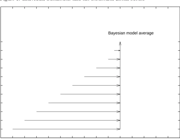
In this way the predictive density is sequentially built up over time. Figure 1 provides a graphic view of the model combination and displays a set of submodels available at
t = 10. The horizontal lines indicate the data used in forming the posterior. The forecasts from each of these submodels, which use different data, are combined (the vertical line) using the submodel probabilities. M11 uses the prior in the event of a
structural break at t = 11. If there has been a structural break at say t = 5, then as new data arrive, M5 will receive more weight as we learn about the regime change.
Continuing in this fashion, the general results are as follows. The predictive density for yt is obtained by integrating across the available submodels:
p(yt|Yt−1) = "t−1 X i=1 p(yt|Yi,t−1, Mi)p(Mi|Yt−1) # (1−λt) +λtp(yt|Yt,t−1, Mt). (7)
The first term on the right-hand side is the predictive density assuming a break occurs prior to timet (or no break at all in the case ofM1) times the probability of no break at
timet. The final term is the probability of a break at time tmultiplied by the predictive density conditional on this break. Therefore, p(yt|Yt,t−1, Mt) with Yt,t−1 ={∅} is based
only on the prior p(θ|Mt). However, future data {yt+1, yt+2, ...}, is used to learn about
the new value of θ for Mt. If λt= 0, then submodel Mt receives no weight.
After observing yt, submodel probabilities can be updated through Bayes’ rule. For instance, p(Mi|Yt) = ( (1−λt)p(yt|Yi,t −1,Mi)p(Mi|Yi,t−1) p(yt|Yt−1) , 1≤i < t λtp(yt|Yi,t−1,Mt) p(yt|Yt−1) i=t. (8) At time t there are a maximum of t submodels that are being entertained. Any feature of the posterior distribution of θ can be calculated by model averaging. For example, if h(θ) is a function of the parameter vector then its expected value is
E[h(θ)|Yt] = t
X
i=1
E[h(θ)|Yi,t, Mi]p(Mi|Yt). (9) Similarly, there are t + 1 submodels that contribute to the predictive density, and if
g(yt+h), h≥1, is a function ofyt+h then11 E[g(yt+h)|Yt] = t X i=1 E[g(yt+h)|Yi,t, Mi]p(Mi|Yt)(1−λt+1) +E[g(yt+h)|Yt+1,t, Mt+1]λt+1.(10)
Note that with the appropriate definition of h(·) and g(·), we can recover any moment of interest or probability. Quantiles can be calculated through simulation. In this case, a draw from the submodel distribution is first taken before a submodel specific feature is sampled such as a parameter or the simulation of a future observation. Collecting a large number of draws and ordering them allows for the estimation of a quantile.
Since submodels are identified with particular start-up points, they represent break points. That is, submodels with high posterior probability identify the most likely structural break points. For example, ifMi has a large probability among all candidate submodels, it suggests the most recent break occurred at timei. The case ofM1 denotes
no structural break while all other submodels denote a break point in-sample. A plot of the distribution of submodels as a function of time may be informative as to when breaks occurs and uncertainty regarding them. Similarly, a time series plot of E[θ|Yt] presents evidence regarding structural change of the parameter θ through time.
Another useful posterior summary measure of structural breaks ismean useful obser-vations (MUO). For instance, if there were 100 data points and submodelM45has a very
11Note that we have implicitly assumed one break occurs over the forecast horizon, however, it is possible that multiple breaks occur att+1, t+2, ..., t+h. This can be accounted for, as in Equation (10), by integrating over all possible break permutations.
high posterior probability, this suggests 55 observations would be useful in estimating
θ associated with the post break model M45. Mean useful observations is a plot of the
expected number of useful observations at a point in time and is calculated at timet as, MUOt=
t
X
i=1
(t−i+ 1)p(Mi|Yt). (11)
In the circumstance where no breaks occur, MUOt as a function of time would be a 45 degree line. However, when a break occurs MUOt drops below the 45 degree line.
2.1
Prior specification
A coherent model of learning requires that the predictive density for each submodel
Mi must be a proper density. In the current context, where the predictive density
p(yt+1|Yi,t, Mi) defined by the mixture in (3) above, this condition will be satisfied if
p(θ|Yi,t, Mi) is a proper density. If at time t, the number of observations since the breakpoint associated with submodel i, that is the difference t −i+ 1 is sufficiently large, then p(θ|Yi,t, Mi) will generally be proper even if the original prior p(θ|Mi) is an improper ’ignorance prior’.
The use of improper priors or even highly diffuse priors is clearly inappropriate here. It may take many observations before p(θ|Yi,t, Mi) is concentrated enough to generate predictive distributions that would receive any significant support. For an econometri-cian who is trying to generate forecasts using available data, there are significant gains in being able to respond more quickly to the possibility that a break may have occurred recently. Our approach is to adopt proper priors. Simulating a model based on the prior, and considering the empirical moments is often helpful in selecting prior parameters.
We find it convenient to use the same form for p(θ|Mi) at each data point in the empirical applications below, but this restriction can be relaxed. For example, the prior
p(θ|Mi), may change through time as the econometrician’s beliefs regarding parameters from a new regime changes. We discuss an example in Section 3 in which the prior
p(θ|Mi) is centered around the most recent posterior mean of the parameter.
Similarly, there is no obvious reason why an analyst should insist on using the same value forλtin every period. If, in his subjective judgment, his model has been producing satisfactory forecasts, and if nothing has occurred that would suggest a recent break, he may choose an extremely low value of λt. On the other hand, if he sees a marked decline in the quality of his forecasts, then he might think it appropriate to set λt at a larger value. In our inflation example below, we found that an ad hoc rule in which λt is modeled as an increasing function on the size of past forecast errors does quite well.
The approach discussed in the previous section can also be adapted to the case where the structural instability of the data-generating process is manifested by changes in the form of the conditional data density itself, as noted above. The simplest way would be to simply introduce more than one data density in each period. Suppose that the analyst believes that if there is a break after period t, there are K possibilities for the
data density12in periodt+1, denoted bypk(y
t+1|θk, Mtk+1), each accompanied by a prior
p(θk|Mk
t+1). Suppose also that the analyst assigns the probabilityλkt+1 to Mtk+1. In this
context, the hypothesis Mt+1, that there was a break immediately following period t,
is defined by Mt+1 ≡ {Mtk+1}Kk=1, and its prior probability is λt+1 = PK
k=1λkt+1. The
predictive distribution conditional on a break, is the mixture
p(yt+1|Mt+1) = K X k=1 ·Z p(yt+1|θk, Mtk+1)p(θk|Mtk+1) dθk ¸ (λk t+1/λt+1).
After yt+1 is observed, the model probabilities p(Mtk+1|Yt+1) and posterior distributions
are updated in the usual way. Note also that there is no reason to restrict attention to the case where the number of potential models is fixed over time.
2.2
Computational issues
For many econometric models, all of the quantities discussed in the previous subsection can be calculated using standard Bayesian simulation methods. For an introduction to Markov chain Monte Carlo (MCMC) see Koop (2003) while Chib (2001), Geweke (1997) Robert and Casella (1999) provide a detailed survey of MCMC methods.
The following steps are required for model estimation at time t:
1. Obtain a sample from the posterior of submodel Mi, i = 1, ..., t+ 1. Calculate posterior quantities for each of the t submodels {Mi}ti=1 or predictive features of
interest for the t+ 1 submodels {Mi}ti=1+1.
2. Calculate submodel probabilities, p(Mi|Yt), i= 1, ..., t.
3. Perform model averaging on quantities of interest, forecasts, etc., using equations (9) and (10). λt+1 coupled with the submodel probabilities from step 2 give the
t+ 1 submodel probabilities used in forecasting.
Typically, and in our applications, we must repeat the above steps for all observations
t = 1, ..., T. However, various schemes in which breaks are permitted at periodic times could be considered by setting the appropriate subset of{λt}Tt=1 to 0.
In the special case of the linear model with a conjugate normal-gamma prior an analytical solution is available for the posterior in Step 1. In other cases, Gibbs or Metropolis-Hasting sampling can be used to obtain a sample from each of the submodel posteriors. There are several approaches that can be used to calculate the marginal likelihood. These include Chib (1995), Gelfand and Dey (1994), Geweke (1994), and Newton and Raftery (1994). For our model in which we do recursive forecasting a predictive likelihood approach is both efficient and accurate and facilitates our updating equations, such as (8).
12In the following we drop conditioning on an empty information setY
2.3
Learning about the arrival rate of structural breaks
The main motivation of this paper is to provide forecasts in an environment where the analyst revises his beliefs about structural breaks with the arrival of non-sample data. In this case, the parameter λtis interpreted as a prior belief whose value will vary as the analyst receives new non-sample information, and past sample data is not informative about λt. In other words, the structural break process is outside of the DGP.
But the framework developed above can be readily adapted to the special case in which the only available information is that contained in the observed data. For example, consider the model in which λt ≡ λ a fixed parameter and breaks occur according to an iid Bernoulli(λ).13 In this case, λ can be interpreted as the arrival rate of structural
breaks, about which the analyst revises his beliefs as new data are observed.
The results in Equations (7) – (10) are now conditional on λ. From (7) we have
p(yt|λ, Yt−1). Using this, the likelihood, as a function of λ is
p(y1, ..., yt|λ) = t
Y
k=1
p(yk|λ, Yk−1). (12)
Note thatp(θ|Yi,t, Mi) is independent of λ and sampling forθ for submodel Mi precedes as before. The data density ofy1, ..., yt given λ is a function of the submodel predictive likelihoods in which all submodel parameter uncertainty has been integrated out.
A natural prior is λ ∼ B(a, b). A simple approach to sampling is a Metropolis-Hasting random walk proposal. Given a previous λ a new candidate can be generated as λ0 = λ+u, where u is a random draw from a symmetric density (ie. u∼ N(0, τ2)).
If p(λ) is the prior, we accept this new draw λ0 with probability min ½ p(y1, ..., yt|λ0)p(λ 0 ) p(y1, ..., yt|λ)p(λ) ,1 ¾ , (13)
and otherwise reject. This gives a set of draws {λ(i)}N
i=1 from the posterior p(λ|Yt). There are a few changes to our previous results. The predictive density for yt+1 must
integrate out λ and is,
p(yt+1|Yt) = Z p(yt+h|λ, Yt)p(λ|Yt)dλ (14) ≈ 1 N N X i=1 p(yt+1|λ(i), Yt) (15) where p(yt+1|λ(i), Yt) is from (7).14 It is straightforward to obtain draws from the pre-dictive density from which moments, quantiles etc. can be computed. To take a draw from p(yt+1|Yt) do the following: take a draw of λ
0
∼ p(λ|Yt), this determines the
13This approach can be readily extended to the case whereλ
tis a function of covariates.
submodel probabilities: p(M1|λ 0 , Yt)(1−λ 0 ), ...., p(Mt|λ 0 , Yt)(1−λ0), λ0, for submodels
M1, ..., Mt, Mt+1, respectively, occurring at time t+ 1.15 Using this discrete distribution
of submodels, randomly draw a submodel Mi0, and then draw a y from the predictive density of that submodel, y ∼ p(yt+1|Yi0,t, Mi0). This last draw is obtained from a)
θ0 ∼p(θ|Yi0,t, Mi0), b)y ∼p(yt+1|Yi0,t, θ 0
, Mi0).
Other quantities, such as the submodel probabilities (8), or the posterior of θ in the break model (9) must be averaged over the draws of {λ(i)}N
i=1.
Another important feature of our model is that all model parameters are subject to change from a break. However, we may want to assume that a break only affects a subset of submodel parameters. This belief can be approximated by calibrating the priors for parameters of new submodels to past data. For example, we could calibrate the prior for regression parameters based on the posterior mean and variance of the structural break model last period. We provide an example of this and the estimation of λ in our application to inflation.
3
Empirical Examples
In this section we present results from simulated data and two examples in macroeco-nomics. In both cases we consider the following linear model,
yt=Xt−1β+²t, ²t∼N(0, σ2) (16) whereytis the variable of interest that is assumed to be related to k regressorsXt−1
avail-able from the information set Yt−1. Independent priors β ∼ N(µβ, Vβ), σ2 ∼IG(v20,s20) rule out analytical results, so we use Gibbs sampling to obtain draws from the pos-terior distribution.16 If θ = [β σ2], then Gibbs sampling produces a set of simulated
draws {θ(j)}N
j=1 from the posterior distribution after discarding an initial burnin period.
In the following examples N = 5000, which are collected and the first 100 draws are dropped. To calculate the marginal likelihood of a model and therefore model probabili-ties through time we use the method of Geweke (1994) which uses a predictive likelihood decomposition of the marginal likelihood. That is,
p(yi, ..., yt|Mi) = t
Y
k=i
p(yk|Yi,k−1, Mi). (17)
Each of the individual terms in (17) can be estimated consistently as
p(yk|Yi,k−1, Mi)≈ 1 N N X j=1 p(yk|θ(j), Yi,k−1, Mi). (18)
15For example, these probabilities areP(M
i att+ 1|λ, Yt) =P(Mi att|λ, Yt)P(no break att+ 1) =
P(Mi|λ, Yt)(1−λ). As beforeMt+1denotes a new submodel from a break out-of-sample,P(Mt+1 att+ 1|Yt) =λ.
16See Koop (2003) for details on posterior sampling for the linear model with independent but con-ditionally conjugate priors.
where {θ(j)}N
j=1 are Gibbs draws from the posterior p(θ|Yi,k−1, Mi). Since we calculate the posterior for all submodels starting from t= 1 and producing forecasts sequentially as we work up to t = T, the predictive likelihood is conveniently calculated at the end of each MCMC run along with features of the predictive density, such as forecasts. Note that it is the individual terms p(yk|Yi,k−1, Mi) that enter directly into the submodel probabilities (8) and the predictive density of the break model. Finally, we found this approach to marginal likelihood computation to be accurate and produce similar results to Chib (1995) and Gelfand and Dey (1994).17
3.1
Change-points in the mean
As a simple illustration of the theory presented, consider data generated according to the following model,
yt = µ1 +²t, t <75 (19)
yt = µ2 +²t, 75≤t <150 (20)
yt = µ3 +²t, t≥150 (21) with µ1 = 1, µ2 = .1, µ3 = .5, ²t ∼ NID(0, .3), and t = 1, ...,200. Priors were set to
µ∼N(0.2,9), σ2 ∼IG(25/2,10/2), λ
t = 0.01 for t= 1, ...,200.
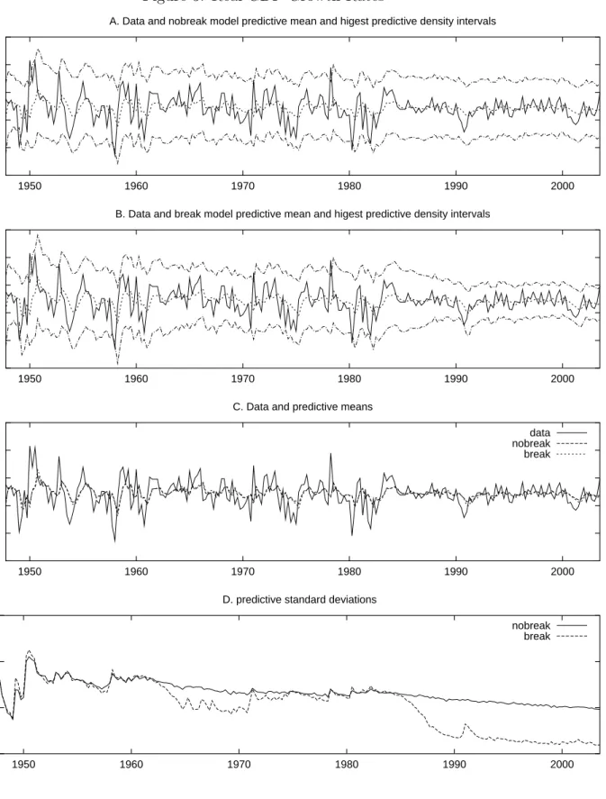
Figure 2 displays a number of features of the model predictions. We compare the break model to a nobreak alternative, both with identical priors.18 Panels A and B show
the predictive mean along with the 95% highest density region (HDR) from the predictive density one period out-of-sample. This interval was obtained through simulation from the predictive density based on 5000 draws, which is described as follows. First, a submodel was randomly chosen based on the submodel probabilities at time t−1, next a parameter vector was sampled from the posterior simulator and used to simulate the submodel ahead one observation. The smallest interval from the ordered set of these draws that has 95% probability gives the desired confidence interval.
Both sets of confidence intervals are similar before the break at t = 75 with the exception of a large positive outlier that the break model briefly interprets as a break. However, after the first break, panel C shows a quick reduction in the predictive mean from the break model while the predictive mean from the nobreak model remains high for a long time. Also note that the density intervals for the nobreak model appear to be uncentered relative to the data after the first break.
Similarly, panel D shows the nobreak model to understate the dispersion in the predictive density just after the first break point. On the other hand, the break model
17For example, for the nobreak model of Section 3.2 with an unrestricted prior, the predictive likeli-hood method gives a log(M L) estimate of -321.263, while Chib method gives -321.271, and Gelfand-Dey -321.272. For the ARCH-in-mean model of Section 3.3 the the predictive likelihood method gives -74.112 while Gelfand-Dey gives -74.210.
18For convenience we label the structural break model as thebreak model and refer to a model that assumes no breaks as thenobreak model.
correctly identifies a break and consequently has a large increase in the uncertainty about future observations. The second break point is much harder to detect and we only observe a gradual increase in the predictive mean, and predictive standard deviation.
These figures suggest that predictions from the break model should be superior to models that ignore breaks. Table 1 show the improvements in terms of forecasting preci-sion and the log marginal likelihood of both models. We include the root mean squared error (RMSE) and mean absolute error (MAE) based on the predictive mean.19
Out-of-sample forecasts are included for all observations.20 Besides the improved forecasts, the
estimates for the log marginal likelihoods indicate a log Bayes factor of 22.6 in favor of the break model.
Finally Figure 2E displays the submodel probabilities through time. This is a 3-dimensional plot of (8), and is the probability of the most recent break point given data up to time t. The model axis displays the submodels, identified by their starting observation. Note that the number of submodels is linearly increasing with time. The submodel probabilities at a point in time can be seen as a perpendicular line from the time axis. At t = 1 there is only one submodel which receives all the probability, at
t= 2 there are 2 submodels etc. It can be seen that up until observation 75 M1 receives
almost probability 1.21 However, after observing the first break at t = 75, the weight
on M75 quickly increases, which allows a fast adjustment to the new data generating
process.22 After this the probability of M
1 drops to zero andM75 continues to receive a
high probability until the latter part of the sample. The difficulty in detecting the final break att= 150 is clearly seen in this figure with the low hump and dispersed submodel probabilities in this region.
In additional experiments, we simulated from a structurally stable model (19) for 200 observations. The break model produced very similar results to a no break model. For instance, from one of the simulations, the RMSE for the predictive means was .5622 for the break model and .5604 for the no break model. Other results were very similar across models. This suggests that the approach can be confidently used even when no breaks are present in the data. The next two subsections consider application to forecasting real output and inflation.
3.2
Real Output
A recent literature, beginning with Kim and Nelson (1999), and McConnell and Perez-Quiros (2000), documents a structural break in the volatility of GDP growth (see Stock and Watson (2002) for an extensive review). We consider model estimates and forecasts
19Based on a quadratic loss function the predictive mean is the Bayes optimal predictor.
20The 1st prediction is based only on the prior. Evaluating forecasts based on data in the latter half of the sample, for this example and others, produced the same ranking among models.
21From the figure it can just be seen that there is a one time spike in M
64 at observation t = 64 associated with a positive outlier of 2.8456 previously mentioned.
22For instance, based on data up to observation 80,M
75, M76, andM77have probabilities, 0.35, 0.12, and 0.11 respectively. By observation 90 these figures are 0.57, 0.18, and 0.14.
from an AR(2) in real GDP growth. Let yt = 100[log(qt/qt−1)−log(pt/pt−1)] where qt is quarterly U.S. GDP seasonally adjusted and pt is the GDP price index. Data range from 1947:2 - 2003:3, for a total of 226 observations. The model is
yt =β0+yt−1β1+yt−2β2+²t, ²t∼N(0, σ2). (22) Realistic priors were calibrated through simulation23 and are µ
β = [.2 .2 0]0, Vβ = Diag(1 .03 .03), v0 = 15, s0 = 10.24 We set λt = .01, t = 1, ...,226 which implies an expected duration of 25 years between breaks points The results presented impose stationarity; removing this constraint produces similar results.
Figures 3 - 5 display several features of the estimated model, and Table 2 reports out-of-sample forecasting results. Panels A and B of Figure 3 present the data along with the predictive mean and the associated HPD interval for the break and nobreak AR(2) model, both with the same prior specification. Both models produce very similar predictions as can be seen in panel C of this figure. However, the confidence interval from 1990 onward is noticeably narrower for the break model. The differences in the predictive standard deviations are easily seen in Figure 3D. There is a clear reduction in the standard deviation beginning from the end of the 1980s for the break model, as well as a less pronounced reduction in the 1960s. In contrast the nobreak model estimates the predictive standard deviation as essentially flat with only a slight reduction over time.
The evidence for structural breaks can be seen in Figure 3E. For instance, there is some weak evidence of a break in the 1960s, however as we add more data the probability for a break during this period diminishes. Notice, however, that from the 1960s on, there is always some uncertainty about a break as new submodels are introduced. This can be seen from the small ridges on the 45 degree line between Submodels and Time. The final ridge in this plot is associated with a break in 1983:3. This is more clearly seen in Figure 4 which shows the very last line of the submodel probabilities in Figure 3E based on the full sample of data. There is some uncertainty as to when the break occurs with the maximum probability being associated with submodel 1983:3. Kim and Nelson (1999), and McConnell and Perez-Quiros (2000) find evidence of a break in 1984:1.25
Figures 5A and 5B plot the evolution of the unconditional first and second moment implied by the model. The estimates are computed using the available information at each point in time and therefore reflect learning about structurally stable model parameters and structural breaks. The unconditional mean shows some variability but
23When we simulated artificial data using this prior, the 95% confidence regions for the unconditional mean, standard deviation, and the 1st order autocorrelation coefficient are (-2.05,2.71), (0.64,1.27), and (-0.10,.52) respectively.
24The priors are conservative, but not unduly so. The proportion of realized observations that lie within the predictive density 95% confidence region, when the posterior always equals the prior, is 0.978. 25There are of course some important methodological differences between their work and our ap-proach. Kim and Nelson (1999) use Bayesian methods but only consider one break while McConnell and Perez-Quiros (2000) is based on the asymptotic theory of Andrews (1993) and Andrews et al. (1996).
mostly stays around 1. In other words, the structural breaks do not appear to affect the long-run growth properties of real GDP. In contrast, Figure 5B shows 3 distinct regimes in the unconditional variance. Ignoring the transition periods, the unconditional variance values are 1.8 (1951-1962), 1.2 (1965-1984), and .40 (1990-2003). Rather than a one time break in volatility, our results point to a gradual reduction in volatility over time with evidence of 3 separate regimes.
Table 2 displays out-of-sample results for one-period ahead forecasts. In addition to a quadratic loss function, optimal forecasts are computed for the linear exponen-tial (LINEX) loss function discussed in Zellner (1986). This loss function, L(y,yˆ) =
b[exp(a(ˆy− y))−a(ˆy−y)−1] where ˆy is the forecast and y is the realized random variable ranks overprediction (underpredictions) more heavily for a > 0 (a < 0). The table includes b = 1 with a = −1, and a = 1. We report the MAE and RMSE for the predictive mean and for the probability of positive growth next period,I(yt+1>0),
whereI(yt+1 >0) = 1 ifyt+1 >0 and otherwise 0.26 Based on our previous discussion it
is not surprising that the MAE or RMSE for both models are very close; neither of these two criteria are affected by the possibility that the predictive variance might be unstable. When the LINEX loss function is used, the break model’s ability to capture variations in higher moments provides small gains. On the other hand, the break model produces a 10% reduction in the MAE when forecasting future positive growth as compared to the nobreak model. We also computed longer horizon forecasts (not reported) which provide a similar ranking among the 2 models. Finally, estimates for the log marginal likelihoods indicate a log Bayes factor of 15.6 in favor of the break model.
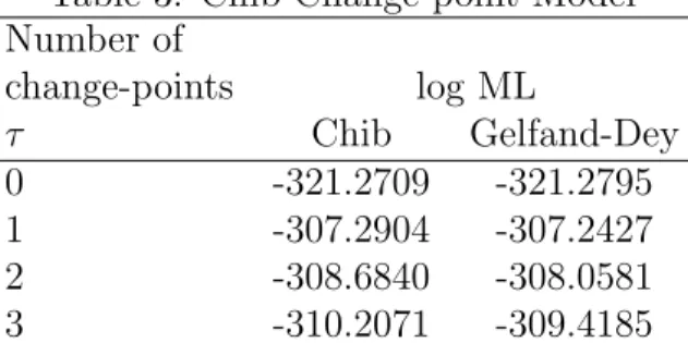
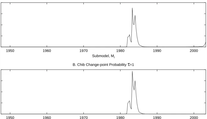
As a check on our analysis, Tables 3 and 4 display the results using the Chib (1998) change-point model. This approach uses a first-order Markov switching model with a specific structure on transition probabilities. Testing for the number of regimes m, is then a test for the number of structural breaks. The m-state (m ≥ 1) model which allows for τ =m−1 breaks is
yt = β0,st +yt−1β1,st+yt−2β2,st +²t, ²t∼N(0, σst2), st= 1,2, ..., m, (23)
P(st=i|st−1 =i) =pi, P(st=i+ 1|st−1 =i) = 1−pi, 1≤i < m, (24)
P(st=m|st−1 =m) = 1. (25)
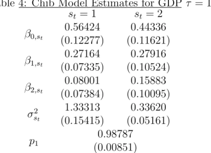
where each 0 < pi < 1. We allow all parameters to break and use the same priors as above for regression parameters andpi ∼Beta(20,1),i= 1, ..., τ, which favors infrequent breaks. Table 3 displays full sample estimates of the marginal likelihood based on Chib (1995) and Gelfand and Dey (1994) methods. Both produce similar results and suggest at least 1 break has occurred. The model estimates associated with 1 break are found in Table 4 and are consistent with our previous results indicating a break in volatility. The first regime implies an unconditional variance for GDP growth of 1.47 while for the second regime it is 0.39. The posterior density of the break point is plotted in Figure 4B, and shows a close correspondence to our model. In summary, our approach
26E
to forecasting in the presence of breaks produces similar results to existing methods based on full sample estimation.
3.3
Inflation
Another well-known economic relationship that exhibits structural breaks is the Phillips curve, which in its most basic form posits a negative relationship between inflation and unemployment. This structural model has motivated a number of empirical studies that forecast inflation, and many have questioned the stability of this relationship (see Stock and Watson (1999) and references therein). It is therefore of interest to see if we can exploit information from this relationship in the presence of model instability.
Define quarterly inflation as πt= 100 log(pt/pt−1), where pt is the GDP price index, and consider the following model for predicting h-period ahead inflation
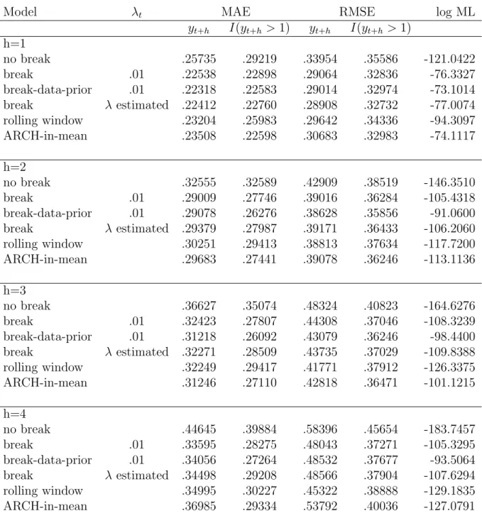
πt+h =β1+πtβ2+ytβ3+Utβ4+²t+h, ²t+h ∼N(0, σ2) (26) whereytis the growth rate of real GDP, Utis the unemployment rate, and h= 1,2,3,4. The benchmark prior is µβ = [.5 .5 0 0]0, Vβ = Diag(1 .2 .1 .1), v0 = 15, s0 = 5, λt =
.01.27 Table 5 reports out-of-sample forecasting performance, while Figure 6 displays
predictive features of the models, submodel probabilities, and Figure 7 records the model parameter estimates through time.
Panels A – C of Figure 6 show the predictive mean and associated predictive density regions for the break and nobreak models withh = 4. As expected, both models clearly lag in responding to inflation, but the break model tends to produce a tighter density interval during the 1960s and 1990s. Panel B also shows that the break model does better in adjusting to the increase in inflation during the 1970s following the oil shock. Note also that the forecasts from the nobreak model in panel A hardly responds during this period. The success of the break model lies in the identification of a break in the process at 1972, as seen in panel D. For instance, based on observations through to 1973, submodels associated with 1972:1, 1972:2, and 1972:3 receive probabilities of 0.62, 0.13, and 0.12, respectively. In other words, the economist in 1973 has learned that the probability that a break recently occurred is high. Other breaks occur around 1950:2 as a result of the increase in primary commodity prices and the outbreak of the Korean war, and during the 1981-82 recession that followed the Federal Reserve’s decision to target the rate of growth of the monetary base.28
Figure 6:C also includes a structural break model in which the prior on the variance of each submodel is calibrated to past data. The model is labeled break-data-prior and discussed below. Even in the presence of a break there may be benefits to using data prior to the break. The model captures this idea and the predictive standard deviation
27This prior specification provides a very conservative predictive density: the proportion of realized observations that lie within the predictive density 95% confidence region, when the posterior always equals the prior is 1, forh= 1, ...,4.
is often lower than the structural break model with benchmark priors. The model also provides good forecasts.
The implications for parameter change due to the 3 main breaks that we have iden-tified are found in Figure 7. This figure reports the posterior mean of the break model parameter and the nobreak model parameter as a function of time. The most significant changes in the parameters appear to be a temporary increase in the intercept, accom-panied by a decrease in the coefficient on unemployment. Estimates for the variance coefficient σ2 increase during the episodes of high inflation, but generally show a
down-ward trend. In addition, there has been a gradual increase in the importance of lagged inflation,β2, which by the end of the sample achieves a value of 0.5. Except for the early
part of the sample there is very little evidence that real growth rates or unemployment are important factors in predicting inflation. There appear to be substantial differences in the parameters for the break and nobreak models. These differences help explain why accounting for breaks is important and we now consider how they effect forecasts.
Table 5 illustrates the benefits of explicitly dealing with these structural breaks. We include several comparison models besides the nobreak model.29 The first is an identical
structural break model except that it sets the prior onσ2 for each new submodel centered
on the most recent posterior mean of σ2. Using the IG(ν
0/2, s0/2) prior we set s0 =
Et−1[σ2](ν0−2), ν0 = 5 for submodelMtwith a prior for regression parameters discussed above. This specification makes use of past data as a starting point for learning.30
The next model assumes the probability of a break is Bernoulli(λ), and is estimated from past data following Section 2.3. Here we use the benchmark prior for submodel parameters and an informative prior λ ∼B(.05,20) which favors infrequent breaks. At each point in the sample λ is estimated along with other submodel parameters and incorporated into forecasts. The final estimate of λ is generally small with posterior mean (stdev) ranging from 0.02(0.01) to 0.005(0.005) for different h.
A third comparison is a model estimated from a rolling window of data. That is, the model uses the most recent 50 observations for estimation and forecasting, is assumed to be structurally stable and has an identical prior specification. A rolling window estimate is an ad hoc, but frequently useful way of dealing with structural breaks, and is popular in economics and finance. A final competitor is a parsimonious ARCH-in-mean model which captures a link between inflation volatility and levels. It has the form,
πt+h = β1 +πtβ2+σt2+hγ+²t+h, ²t+h ∼N(0, σ2t+h) (27)
σ2
t+h = ω+α²2t+h−1. (28)
We use identical priors for β1, and β2 and setω ∼Gamma(0.1,1), α∼Beta(1,6)I(α <
29A previous version of this paper found that modeling the subjective probability of a break as an increasing function of the standardized forecast error observed in the previous period improved forecast precision.
30We found it important to allow for a more diffuse prior through a smaller ν
0 as compared to the previous setting of ν0 = 15. The improvements from this model are not due to this change since the nobreak case withs0= 5, ν0= 5 has marginal likelihood values of -127.28, -151.49, -168.75, -187.20 for
1/√3), which imposes a positive fourth moment, and γ ∼ N(0,1). To estimate this model we used a random walk Metropolis-Hasting routine with a fat-tailed proposal density. The model is estimated and out-of-sample forecasts computed conditional on
Y0,t, t = 0, ..., T. All parameters are sampled jointly and we use the previous poste-rior output to calibrate the covariance matrix of next period’s proposal density. This covariance matrix was scaled to target an acceptance rate of 40-50%. The approach provided an efficient and automatic way of calculating model estimates and forecasts through time. The marginal likelihood estimate was based on the predictive likelihood decomposition.
The out-of-sample forecasts begin at 1965:1 and are based on information available at time 1965:1 - h. For each forecast horizon h = 1, ...,4, the structural break model improves on the MAE and RMSE of the nobreak model. In addition to forecasts of
yt+h, we report forecasts of I(yt+h > 1), which on an annual basis is the probability of inflation being in excess of 4%: this may be a useful indicator of high inflation and a quantity of interest to policy makers.
There are significant gains - in both MAE and RMSE - in using either of the break model or the rolling window model to forecast yt+h and I(yt+h > 1) at all forecast horizons considered here. Furthermore, the log Bayes factors - which range between 40 and 80 in favor of the break model - indicate that the data provide overwhelming evidence against the hypothesis that the relationship in (26) is stable over time. In addition, the evidence based on the marginal likelihoods is very strong for the break model compared to the rolling window model. The ARCH-in-mean model performs well in terms of point forecasts, however based on the marginal likelihood it is generally dominated by the structural break specifications. The break model with λ estimated produces similar results to the case when λt is preset to .01. Overall, the best performance comes from the structural break model where the prior on σ2 is calibrated using past data.31 This
model has the best marginal likelihood and competitive forecasts for each horizonh. We did explore other rolling window models which condition on a different length of historical data. Generally, there were improvements in some directions and a worsening in others. The reason for this is that a fixed window of data is not optimal. To see this, consider Figure 8 which plots the mean useful observations for h = 4. Recall, from Section 2 that MUOt is the expected number of past data points that is useful in estimation and forecasting at a particular point in time. The 45 degree line in this figure is for the model that gives equal weight to all observations. The horizontal line at 50 is the rolling window estimator. The MUOt implied by the break model varies over the sample considerably. Sometimes we should be using more than 50 observations while at other times much less. According to our model the optimal number of useful observation varies over time.
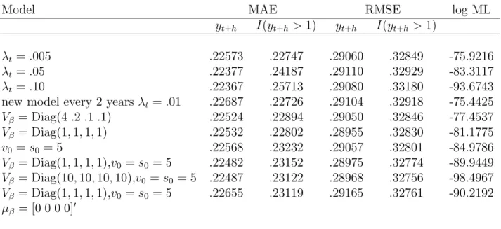
Finally, Table 6 displays a sensitivity analysis for h = 1 with different prior as-sumptions on the original break model. Similar results were found for the other cases,
31Other specifications in which regression parameter priors were calibrated to past data produced minor improvements.
h = 2,3,4. The forecast improvements are quite robust for a range of different priors. However, the marginal likelihood displays some variation. Generally, the approach de-teriorates if new models are continually introduced with a high prior probability (see
λt =.10 case) since the benefits to learning about a structurally stable relationship are lost by incorporating noise from new models. Secondly, the results are worse when the prior on the model parameters is more diffuse (seeV = Diag(10,10,10,10),v0 =s0 = 5) .
Intuitively, it takes longer to learn about structural breaks in this situation. Therefore, our approach can be expected to perform well with sensible informative priors and a prior break probability that is not too large.
There are situations where it may be desirable to have a high temporary break probability. For instance, as discussed in the Introduction, the economist who feels that the Phillips curve will become unstable in the 1970s as a result of new economic theory, may want to set a high λt for a few years before returning it to a low value. How the prior affects the results is not clear and would need to be studied on a case by case basis.
4
Discussion
This paper provides an approach to dealing with structural breaks for the purpose of model estimation, inference and forecasting. We focus on the case in which the break probability is a subjective parameter and possibly a function of non-sample data, as well as the case when break arrival is fully specified as an iid Bernoulli distribution. We make a particular emphasis on careful prior elicitation; the focus of interest when specifying priors should be their implications for the predictive distribution of observables. The form of these priors can vary over time, as the analyst learns more from non-data based sources, or can be set based on past posterior moments. Developing tools for prior elicitation in various forecasting contexts along the lines of the extensions discussed in Section 2.1 will be the subject of future research.
There are also numerical issues that will have to be addressed. In our examples, the number of submodels is equal to the sample size, but the computational burden is quite modest: computing all the results (including the HPD regions) reported for GDP growth rates took just under 25 minutes on a modern Pentium chip based computer. Of course for forecasting in real time, only the submodels available at time t (in our case, t+ 1 models) need to be estimated at timet, and importance sampling techniques may further reduce these computations by efficiently using past draws from the posterior simulator (Geweke (1994)). In other settings, such as in finance or labor econometrics, the datasets are much larger, and it may be impractical to entertain such a large number of models. In this case, allowing for periodic breaks to occur - for example, at a seasonal frequency - may be a practical alternative.
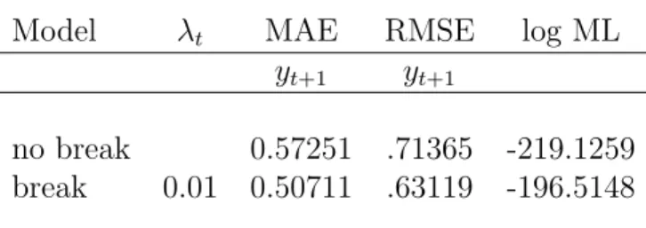
Table 1: Simulation Example
Model λt MAE RMSE log ML
yt+1 yt+1
no break 0.57251 .71365 -219.1259
break 0.01 0.50711 .63119 -196.5148
This table reports mean absolute error (MAE), and root mean squared error (RMSE) for the predictive mean forecast one-period ahead, and the log marginal likelihood estimate. The out-of-sample period is based on all 200 observations.
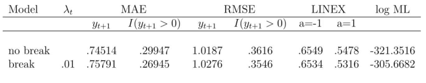
Table 2: Out-of-Sample Forecasting Performance for US Real Output
Model λt MAE RMSE LINEX log ML
yt+1 I(yt+1 >0) yt+1 I(yt+1 >0) a=-1 a=1
no break .74514 .29947 1.0187 .3616 .6549 .5478 -321.3516
break .01 .75791 .26945 1.0276 .3546 .6534 .5316 -305.6682
This table reports mean absolute error (MAE), and root mean squared error (RMSE) for the forecasts based on the predictive mean for one-step ahead real GDP growth
yt+1, and the positive growth indicator,I(yt+1>0), whereI(yt+1>0) = 1 ifyt+1>0 and otherwise 0. In addition average LINEX loss function is reported withb= 1, as well as the log marginal likelihood estimate. The out-of-sample period ranges from 1947:4-2003:3 (224 observations).
Table 3: Chib Change-point Model Number of change-points log ML τ Chib Gelfand-Dey 0 -321.2709 -321.2795 1 -307.2904 -307.2427 2 -308.6840 -308.0581 3 -310.2071 -309.4185
This table displays the full sample marginal likelihood estimates for the Chib change-point model assuming an AR(2) for real GDP growth. τ is the number of change-points and the two other columns are 2 alternative estimates (Chib (1995) and Gelfand and Dey (1994)) of the logarithm of the marginal likelihood.
Table 4: Chib Model Estimates for GDP τ = 1 st = 1 st = 2 β0,st (0.12277)0.56424 (0.11621)0.44336 β1,st (0.07335)0.27164 (0.10524)0.27916 β2,st (0.07384)0.08001 (0.10095)0.15883 σ2 st 1.33313 (0.15415) 0.33620 (0.05161) p1 (0.00851)0.98787
This table reports the posterior mean and posterior standard deviation (in parenthe-ses) for a 2 state change-point model with transition probabilityp1.