https://doi.org/10.1007/s10489-017-1093-y
Scalable aggregation predictive analytics
A query-driven machine learning approach
Christos Anagnostopoulos1·Fotis Savva1·Peter Triantafillou1
Published online: 12 December 2017
© The Author(s) 2017. This article is an open access publication Abstract We introduce a predictive modeling solution that provides high quality predictive analytics over aggregation queries in Big Data environments. Our predictive method-ology is generally applicable in environments in which large-scale data owners may or may not restrict access to their data and allow only aggregation operators likeCOUNT to be executed over their data. In this context, our method-ology is based on historical queries and their answers to accurately predict ad-hoc queries’ answers. We focus on the widely used set-cardinality, i.e., COUNT, aggregation query, asCOUNTis a fundamental operator for both inter-nal data system optimizations and for aggregation-oriented data exploration and predictive analytics. We contribute a novel, query-driven Machine Learning (ML) model whose goals are to: (i) learn the query-answer space from past issued queries, (ii) associate the query space with local lin-ear regression & associative function estimators, (iii) define query similarity, and (iv) predict the cardinality of the answer set of unseen incoming queries, referred to the Set Cardinality Prediction (SCP) problem. Our ML model incor-porates incremental ML algorithms for ensuring high qual-ity prediction results. The significance of contribution lies in that it (i) is the only query-driven solution applicable over general Big Data environments, which include restricted-access data, (ii) offers incremental learning adjusted for
Christos Anagnostopoulos
[email protected] Peter Triantafillou
1 School of Computing Science, University of Glasgow, Glasgow G12 8QQ, UK
arriving ad-hoc queries, which is well suited for query-driven data exploration, and (iii) offers a performance (in terms of scalability, SCP accuracy, processing time, and memory requirements) that is superior to data-centric approaches. We provide a comprehensive performance eval-uation of our model evaluating its sensitivity, scalability and efficiency for quality predictive analytics. In addition, we report on the development and incorporation of our ML model in Spark showing its superior performance compared to the Spark’sCOUNTmethod.
Keywords Query-driven predictive analytics·Predictive modeling·Aggregation operators·Set cardinality prediction·Regression vector quantization· Self-organizing maps
1 Introduction
Recent R&D efforts in the modern big data era have been dominated by efforts to accommodate distributed big datasets with frameworks that enable highly quality and
scalabledistributed/parallel data analyzes. Platforms such as MapReduce [14], Yarn [29], Spark [32] and Mahout [22] are nowadays commonplace. Predictive modeling [26], [23] and exploratory analysis [2,3,6,20] are commonly based on statistical aggregation operators over the results of explo-ration queries [4, 7]. Such queries involve large datasets (which may themselves be the result of linking of other different datasets) and a number of range predicates over multidimensional data vectorial representation, structured, semi- and unstructured data. High quality query-driven data exploration and quality modeling is becoming increasingly important in the presence of large-scale data since accu-ratelypredicting aggregations over range predicate queries
is a fundamental data exploration task [12] in big data sys-tems. Frequently, data analysts, data scientists, and statisti-cians are in search of approximate answers to such queries over unknown data subspaces, which supports knowledge discovery and underlying data function estimation. Imag-ine exploratory and predictive analytics [9] based on a
streamof such aggregation operators over data subspaces being issued, until the scientists/analysts extract sufficient statistics or fit local function estimators, e.g., coefficient of determination, product-moment correlation coefficient, and multivariate local linear approximation over the subspaces of interest.
In modern big data systems like Spark [32], often data to be analyzed possibly extends over a large number of feder-ated data nodes, perhaps even crossing different administra-tion domains and/or where data owners (nodes) may only permit restricted accesses (e.g., aggregations) over their data. Similarly, in the modern big data era, large datasets are often stored in the Cloud. Hence, even when access is not restricted, accesses to raw data needed to answer aggregate queries are costly money-wise. Quality predictive model-ing solutions which are widely applicable, even in such scenarios, are highly desirable.
Consider ad-dimensional data spacex∈Rd.
Definition 1(Range Query) Let ad-dim. box be defined by two boundary vectors[a1, . . . , ad]and[b1, . . . , bd], ai≤bi,ai, bi∈R. A range query is represented by the 2d -dimensional vectorq= [a1, b1, a2, b2, . . . , ad, bd]where aiandbiis lower and higher value, respectively, for thei-th dimension. Queryqis a hyper-rectangle with faces parallel to the axes.
Definition 2(Query Distance)1The normalized Euclidean distance between queries q and q is q − q2 =
1 √ 2d d i=1 ai−ai2+bi−bi2, where √1 2d is a normal-ization factor since 0≤ q−q2≤
√ 2d.
Definition 3(Answer Set Cardinality) Given a range query
q and a dataset B of data points x ∈ Rd,y ∈ Nis the cardinality of the answer set of thosex∈Bin the interior of the hyper-rectangle defined by queryqsatisfyingai≤xi≤ bi,∀i.
The reader could refer toAppendixfor a nomenclature. The reason we focus on theCOUNTaggregation operator is that the answer Set Cardinality Prediction (SCP) of a mul-tidimensional range query is a fundamental task, playing a
1When dealing with mixed-type data points, e.g., consisting of cate-gorical & continuous attributes,we can adopt other distance metrics; this does not spoil the generality of our solution.
central role in predictive modeling. With multidimensional range queries, analysts define the subspaces inRdof interest within the overall data space. High quality cardinality pre-diction in such subspaces then becomes important for data mining, data exploration, time series analysis, and big data visualization tasks [9,12] of data (sub)spaces of interest.
In predictive modeling, data scientists routinely define specific regions of a large dataset that are worth explor-ing and wish to derive and accurately predict statistics over the populations of these regions. This amounts to the SCP of the corresponding range queries. In addition to being an important aggregation operator, in database systems accurate cardinality prediction (which amounts to the well known selectivity estimation problem) is explicitly used for query processing optimization, empowering query optimiz-ers to choose, for instance, the access plan which produces the smallest intermediate-query results (which have to be retrieved from disks and communicated over the network) saving time, resource waste, and money (e.g., in Clouds). Furthermore, SCP is a core operator in modern big data frameworks. Notably, in Spark [32] one of the five funda-mental actions defined is the so-calledcountaction, which is executed over the underlying raw data at each data node.
1.1 Motivation & research objectives
Well-established and widely adopted techniques for Approximate aggregation-Query Processing (AQP) based on sampling, histograms, self-tuning histograms, wavelets, and sketches [13] have been proposed. Their fundamental and naturally acceptable assumption is that the underlying data are always accessible and available, thus it is feasi-ble to create and maintain their statistical structures. For instance, histograms [15] require scanning of all data to be constructed and being up-to-date; the self-tuning his-tograms [1] require additionally the execution of queries to fine tune their statistical structures; the sampling methods [16] execute the queries over the sample to extrapolate the cardinality prediction result.
Consider now a big data environment, where a feder-ation of data nodes store large datasets. There are cases where the data access to these nodes’ data may be either restricted, (e.g., government medical and DNA databases and demographic and neighborhood statistic datasets). Fur-thermore, many real-world large-scale data systems may limit the number of queries that can be issued and/or charge for excessive data accesses. For example, there may exist per-IP limits (for web interface queries) or per developer key limits (for API based queries). Even when the (daily) limit is high enough, repeated executions actually have high mone-tary cost (e.g., in cloud deployments), waste communication overhead due to remote query execution, and computational resources. The accessed data nodes can either fully execute
the queries (to produce exact results) or locally deploy an AQP technique to produce estimates. In the latter case, we must rely upon the SCP accuracy provided by the applied traditional AQP technique. Hence, the cardinality prediction accuracy is upper bounded by the predictability capability of the AQP method.
The above discussion raises the following desiderata: it is important to develop quality AQP techniques that: – D1: are applicable to all data-environment scenarios
(restricted-access or not),
– D2: are inexpensive, i.e., avoid relying on excessive querying of and communication with the data nodes, while
– D3: offeringhigh prediction accuracy, and
– D4: being prudent in terms of compute-network-store resource utilization.
Let us consider an indicative baseline solution for AQP in our environment. One approach is to store, e.g., locally to a central node, all the AQP structures (e.g., histograms, sam-ples, sketches, etc.) from a federation of data nodes. Thus, we can simply locally access this node for SCP. Firstly, this violates our first desideratum, as privacy issues emerge (data access restrictions). Obviously, retaining all AQP structures, provides one with thewholevaluable information about the underlying data (e.g., in the case of histograms, we obtain the underlying probability data distributionp(x), while in sampling methods we retain actual samples from the remote datasets). Even, in cases where the local accesses to AQP structures were secured (which is again subject to major security concerns), we would have to cope with the prob-lem of AQP structure updates. The maintenance of those structures in the face of updates demands high network bandwidth overhead, cost for data transfer (in a Cloud set-ting), latency for communicating with the remote nodes during updates of the underlying dataset at these nodes, and scalability and performance bottleneck problems arise at the central node. Therefore, this approach does not scale well and can be expensive, violating our 2nd and 3rd criteria above.
An alternative baseline solution would be to do away with the central node and send the query to the data nodes, which maintain traditional AQP statistical structure(s) and send back their results to the querying node. As before, this violates many of our desiderata. It is not applicable to restricted-access scenarios (violating criterion 1) and involves heavy querying of the data node (violating crite-ria 2 and 4). Even if this was the case (by violating critecrite-ria 1, 2, and 4), the construction and maintenance of an AQP structure would become a prohibited solution; we struggle with huge volumes of data (data universe explosion phe-nomenon; imagineonlythe creation of a multidimensional histogram over 1 zettabyte). These facts help expose the
formidable challenges to the problem at hand, (a signifi-cant problem for large-scale predictive analytics) which to the best of our knowledge, has not been studied before. In this work we study a query-driven SCP in a big data system taking into consideration the above-mentioned desiderata. Although significant data-centric AQP approaches for car-dinality prediction have been proposed [13] a solution for our intended environments of use is currently not available. There are three fundamental pressures at play here. The first pertains to the development of a solution for cardinal-ity prediction that isefficient, and scalable, especially for distributed scale-out environments, wherein extra commu-nication costs, remote invocation techniques, and estimation latency are introduced. The second pertains to thequality
of cardinality prediction results in terms of accuracy and model fitting, where as we shall see traditional solutions fall short. The third concerns the wide-applicability of a proposed method, taking into account environments where data accesses may be restricted, We propose a solution that addresses all these tensions. Conceptually, its fundamental difference from related works is that it isquery-driven, as opposed to data-driven, and is thus based on a ML model (trained by a number of queries sent to a data node) and later utilized to predict answers to new incoming queries.
The challenging aim of our approach is to swiftly pro-vide cardinality prediction of ad-hoc, unseen queries while (i)avoiding executing them over a data node, saving com-munication and computational resources and money, and (ii) not relying on any knowledge on thep(x), and any knowl-edge about nodes’ data. Through our query-driven SCP, an inquisitive data scientist, who explores data spaces, issues aggregate queries, and discovers hidden data insights, can extract accurate knowledge, efficiently and inexpensively.
1.2 Related work
Given ad-dim. data spacex∈Rdthe holy grail approaches focus on: (i) inspecting the (possibly huge) underlying dataset and estimate the underlying probability density function (pdf) p(x). Histograms (typically multidimen-sional) as fundamental data summarization techniques are the cornerstone, whereby the estimation of p(x)is highly exploited for SCP of range queries, e.g., [1, 15]. The tra-ditional methods of building histograms do not scale well with big datasets. Histograms need to be periodically rebuilt in order to update p(x) thus, exacerbating the overhead of this approach. Central to our thinking is the observa-tion that a histogram is constructed solely from data, thus obviously being not applicable to our problem for the above-mentioned reasons. Histograms are also inherently unaware on the cardinality prediction requests, i.e., query patterns. Their construction method rely neither on query distribu-tionp(q)nor on jointp(q, y)but only onp(x). As a result,
such methods do not yield the most appropriate histogram for a givenp(q)[11]. The limitations of this method are also well-known [27,30].
To partially address some of the above limitations, prior work has proposed self-tuning histograms (STHs) e.g., [1, 27]. The STHs learn a centrally stored dataset from scratch (i.e., starting with no buckets) and rely only on the cardinal-ity result provided by the execution of a query, referred to as Query Feedback Records (QFR). STHs exploit the actual cardinality from QFR and use this information to build and refine traditional histograms. Formally, given a queryqover data with cardinalityy, the methods of STHs estimate the conditionalp(x|y,q)since the main purpose is to construct and tune a histogram conditioned on query patterns. Fun-damentally, the limitations in STHs in our problem stem from the fact that they estimatep(x|y,q), thus, having to data access (in multidimensional STHs, at least one scan of the setBis required), deal with the underlying data dis-tribution and make certain assumptions of the statistical dependencies of data.
Other histogram-based cardinality prediction methods utilize wavelets [31] or entropy-based [28]; the list is not exhausted. Briefly, the idea is to apply wavelet decomposi-tion to the dataset to obtain a compact data synopsis based on the wavelet coefficients. By nature, wavelets-based AQP relies on the synopsis construction over data thus could not be applied to our problem. Overall, STHs and the other advanced histogram-based approaches, are associated with data access for estimating p(x) or any other p(x|q, . . .) thus not applicable in our problem. Sampling methods [16] have been also proposed for SCP. They share the common idea to evaluate the query over a small subset of the dataset and extrapolate the observed cardinality. Finally, another approach for AQP answering to SCP is data sketching; we refer the reader to [13] for a useful survey of sketching techniques. Sketching algorithms construct estimators from the raw data and yielding a function of these estimators as the answer to the query. Therefore, as discussed above, we neither have access to data nor to a sample of them, thus yielding the data sketching and sampling methods inapplicable to our problem.
In conclusion, the data-centric approaches in related work are not applicable to our problem since they require explicit access to data to construct their AQP structures and maintain them up-to-date. For this reason, our proposed solution to this novel setting is query-driven.
Our model can be highly useful when it is very costly (in time, money, communication bandwidth) to execute aggre-gation operators over the results of complex range queries (including joins of datasets and arbitrary selection predi-cates), when data are stored at the cloud, or at federations of data stores, across different administration domains, etc. And, to our knowledge, it is the only approach that can
address this problem setting. It is worth noting that this paper significantly extends our previous work presented in [5]. The interesting reader could refer to [5] to assess the performance of our solution with respect to traditional data-centeric (AQP) systems for cardinality prediction namely with multidimensional histograms, popular self-tuning his-tograms, and sampling methods. In [5], through comprehen-sive experiments we showed that the query-driven approach, which extracts knowledge from the issued queries and corresponding answers, provides higher cardinality predic-tion accuracy and performance, while being more widely applicable. Based on the scalability and efficiency of this approach, we further generalize our model in [5] and imple-ment generalized ML algorithms within the most popular big data system, Spark. Specifically, the major differences of the proposed generic ML model discussed in this paper with that of our paper in [5] are:
– We propose a generalization of the ML model in [5] by introducing (i) associative local linear regression mod-els for cardinality prediction and (ii) the concept of the coefficients lattice in self-organizing maps statistical learning algorithm;
– We provide the theoretical analysis and convergence of the learning algorithms of the generalized ML model (Theorems 2 and 4);
– We implement our ML model within the Spark system; – We provide comprehensive experiments showing the
quality of predictionof our ML model through a variety of evaluation metrics.
– We experiment with thescalability performanceof our ML model compared with the Spark’sCOUNTmethod for answer-set cardinality estimation.
1.3 Organization
The structure of the paper is as follows: Section2reports on the rationale of our approach and the research chal-lenges for the SCP, while summarizes the contribution and our research outcome. In Section 3, we provide prelim-inaries for unsupervised & heteroassociative competitive statistical learning and the self-organizing maps along with the problem formulation for SCP. Section 4provides the set cardinality learning methodology, the machine learn-ing algorithms over the novel introduced lattice concepts and the fundamental convergence theorems of our neuron-based model. In Section 5 we provide an implementa-tion of our model in the Spark system, while Secimplementa-tion 6 reports on a comprehensive performance and comparative assessment with the build-in SparkCOUNTover real large-scale datasets introducing different experimental scenarios. Finally, Section7concludes the paper with future research directions.
2 Challenges & overview
Our approach is query-driven. The first requirement (and challenge) of our approach is to incrementally learn the query patternsp(q)at any time, thus being able to (i) detect possible changes to user interests on issuing queries and (ii) reason about the similarity between query patterns. The sec-ond requirement (and challenge) is to learn the association
q→ybetween a queryqand its cardinalityy, i.e.,p(y|q), thus being able to predict the cardinality. The third require-ment (and challenge) is to learn such association without relying on the underlyingp(x)which in our case is totally unknown and inaccessible. The fourth requirement (and challenge) is to updatep(q)andp(q, y)based on changes in query patterns and to data. Query distributions are known to be non-uniform, with specific portion of the data space being more popular. However, query patterns change with time, reflecting changes of users interests to exploring dif-ferent sections of the datasets of nodes. Hence, we must swiftly adapt and learn on-the-fly thenew query patterns, updating p(q, y) and p(q). Furthermore, updates on the underlying datasets of nodes can independently occur, alter-ingp(x). We must also deal with such mutations, implying the need to maintain the currentq → yassociation, sub-ject to updates of the underlying data. We require a model to meet the above-mentioned requirements.
2.1 Overview ofCOUNTpredictive learning
Consider a setQ= {(qi, yi)}ni=1of training pairs and a new queryqwith actual resulty. Our major aim is to predict its resultyˆ using onlyQwithout executingq. Let us discuss some baseline solutions:
A first idea is to keep all pairs(qi, yi)and givenqwe find the most similarquery qj with respect to Euclidean distance and predictyˆ = yj, with(qj, yj) ∈ Q. We can also involve thekclosest queries toqand average their car-dinality values, i.e.,k-nearest neighbors regression, as will be further analyzed later. The major problems here are: (i) we must store and search all previous pairs for each new query;Q can be huge. Deciding which pairs to discard is not a trivial task (a new pair might convey useful informa-tion while another new one might be a redundant / repeated query); (ii) when data change (updates on raw data), which impacts the query results, it is not trivial to determine which pairs fromQand how many to update. Even worse, all pairs may need updating; (iii) when query patterns change (new user interests), then there may be many pairs inQthat will not contribute to cardinality prediction (the new queries are actually far distant to the previous ones) or even negatively impact the final result.
To avoid such problems we extract knowledge fromQ as to how query and cardinality depend on each other. We
could cluster similar queries given the Euclidean distance, thus forming a much smaller setL of representative (pro-totype) queriesw with|L| |Q|. For instance,w ∈ L
can be the centroid of those queries from Qw ⊂ Q with
distances from w be the smallest among all other repre-sentatives. However, we are not just interested in clustering
Q. We should partitionQaiming at cardinality prediction. An approach could be to assign to each wi ∈ L a ‘repre-sentative’ cardinality value, e.g., the average cardinality of those queries that belong toQwi. Once this assignment is
achieved, we only keepLand discardQ.
Nonetheless, our requirements include incremental learn-ing of the query space in light of cardinality prediction. We require an adaptive clustering algorithm that incremen-tally, i.e., with only one pass of Q, quantizes Q but also with respect to minimizing the prediction error. Also, the adoption of an on-line quantization algorithm, like on-line k-means is not directly applicable in our case as we don’t wish to simply quantize the query space; we explicitly require quantization of the query spacein light of cardinal-ity prediction. Moreover, on-line regression methods, e.g., incremental regression trees [17], on-line support vector regression [24], could not fulfill all requirements. This is because, we also deal with the fact that queries are con-tinuously observed, conveying the way users are interested in data exploration. The capability of the model to adapt to such changes requires explicit information on accessing the very specific regions of the query patterns space; this is neither easily provided nor supported by incremental regres-sion methods. Moreover, the problem here is not only to adapt to changes on the query patterns but to decide which and how representative(s) or regions of the query patterns space to update upon data and/or query updates.
2.2 Contribution & research outcome
We introduce a novel and scalable Machine Learning (ML) modelMthat incrementally extracts information about the
q→yassociation by learningp(q)and, in parallel,p(y|q). Once trained, modelMpredicts the cardinality of anunseen
query without requesting its execution. The major technical contributions are:
– a prediction error-driven, associative local regression model for predicting the aggregate results of range queries. – theoretical analysis of convergence of our machine learning algorithms over large-scale squared and abso-lute loss minimization.
– implementation of our algorithms in the Spark system. – comprehensive experimental results analyzing the
per-formance of our model and showcasing its benefits vis-`a-vis the data-centric Spark’s COUNT method for set-cardinality estimation.
3 Preliminaries & problem formulation 3.1 Preliminaries
We overview the essentials of our ML model, namely Unsupervised Competitive Learning (UCL) [21] and Het-eroassociative Competitive Learning (HCL) [19].
3.1.1 Unsupervised competitive learning
UCL partitions a query pattern spaceR2d characterized by an unknownp(q),q∈R2d. A prototype orneuronwj rep-resents a local region ofR2d. UCL distributesM neurons
w1, . . . ,wM inR2d to approximate p(q). A UCL model learns aswj changes in response to random training pat-terns. Competition selects whichwj the training patternq modifies. Neuronwj wins if it is the closest (based on 2-norm distanceq−wj2) of theM neurons toq. During the learning phase of UCL, patternsq are projected onto their winning neurons, which competitively and adaptively move around the space to form optimal partitions that mini-mize the quantityq−wj22p(q)dqwith winning neuron
wj:wj−q2=miniwi−q2. The neurons upon at-th training patternqare incrementally updated as follows: wj =β(t )
q−wj
andwi=0, ifi=j, (1) where learning rateβ(t )∈(0,1]slowly decreases with the update step.
3.1.2 Kohonen’s self-organizing maps
Kohonen’s self-organizing maps (SOM) [19] is an advanced variant of a UCL, in whichwjcorresponds to thej-th posi-tion rj = [rj1, rj2] of a 2-dim. square lattice/matrix L (we notatewj ∈ L). In SOM, neurons that are topologi-cally close in the lattice correspond to patterns that are also closein R2d. This way a topographic mapping is learned between query pattern and lattice space. This is achieved by
adapting not only the winner neuronwj of a patternq but also its topographical neighborswito some degree through a Kernel distance function h(i, j;t) over the positions ri and rj of neuronswi andwj in L, respectively. Usually, h(i, j;t)is a Gaussian neighborhood function:
h(i, j;t)=exp −ri−rj 2 2 2ρ2(t) . (2)
Parameterρ(t )is the width of the neighborhood with ini-tial valueρ0defined asρ(t )=ρ0exp(−Ttρ), whereTρ is a constant. A small width value corresponds to narrow neigh-borhood. We obtain SOM through an incremental update rule that adapts all neurons that are topographically close to
wj:
wi=β(t )h(i, j;t) (q−wi) ,∀i. (3) A good choice of β(t ) improves significantly the conver-gence of SOM [19]; usuallyβ(t ) = 1+β(tβ(t−−1)1) withβ(0)= 1. SOM yields a high quality vector quantization from all UCL variants because of producing a structured ordering
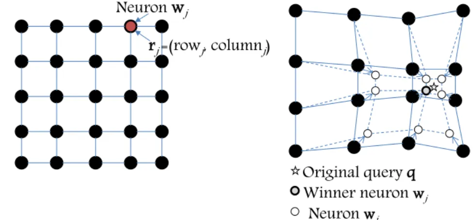
of the pattern vectors, i.e., similar query patterns are pro-jected to similar neurons, making it ideal for our purposes. Figure 1 shows a SOM structure with neuron and posi-tion vectors before and after an update. UCL/SOM does not learn any conditional or joint association between different pattern spaces. In our case, we desire also to estimate an association betweenR2dandN, i.e., estimatep(q, y)with
q∈R2d, y∈N, HCL comes into play.
3.1.3 Heteroassociative competitive learning
HCL estimates indirectly an unknown jointp(q, y), while directly estimates a function f : R2d → Nover random pairs(q, y). In statistical learning theory [21], HCL refers to a function estimation modelM(f, α)(or simplyM) with parameter α ∈ (is a parameter space defined later) for estimating f. The problem of learning M is that of
Fig. 1 aA Self-organizing Map with neuron vectorswjand
position coordinates vectorrj;
bThe adaptation of the self-organizing map after the projection of a query vectorqto its closest neuronwj on the
neurons latticeL
Neuron w
w
jr
j=(row
j, column
j)
Winner neuron
wjNeuron
wiOriginal query qq
choosing from a set of functionsf (q, α),α ∈ , the one which minimizes the risk function:
J(α)=
L(y, f (q, α))dp(q, y), (4)
given random pairs (q, y) drawn according to p(q, y) = p(q)p(y|q)withlossor estimation error L(y,y)ˆ between actual y and predicted yˆ = f (q, α), e.g., L(y,y)ˆ = |y − ˆy|. The goal for HCL is to learn M(f, α0) which minimizes J(α) subject to unknown p(q, y), i.e., α0 = arg minα∈J(α).
3.1.4 Stochastic gradient descent
Stochastic gradient descent (SGD) is considered to be one of the best methods for large scale loss minimization and has been experimentally and theoretically analyzed by [10]. Upon the presence of at-th pattern(q, y),α(t)is updated by:
α(t)= −β(t )∇L(y,yˆ;α(t)), (5)
where∇Lis the gradient ofLatt-th pattern w.r.t.α(t).
3.2 Problem formulation
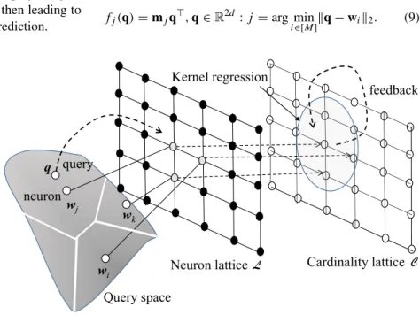
Consider a modelMthat estimates thecardinality predic-tion funcpredic-tion
f :R2d →N
given a finite setQof training pairs(q, y)drawn from the unknownp(q, y), i.e.,y=f (q). The modelMlearns the mapping from query pattern space to cardinality domain by minimizing the risk functionJ(α)in (4) with respect to a
loss function(prediction error)L(y,y)ˆ . A loss function can be, e.g.,λ-insensitiveL(y,y)ˆ =max{|y− ˆy| −λ,0}, λ > 0, 0–1 lossL(y,y)ˆ = I (y = ˆy)withI be the indicator function, squared loss(y− ˆy)2,or absolute|y− ˆy|.
The fundamental problem of the ML model for cardinal-ity prediction is:
Problem 1 Given a datasetBand training pairs of queries and their answer-set cardinality values(q, y) ∈ Q, incre-mentally train a modelMwhich minimizesJ(α).
4 Set cardinality predictive learning 4.1 Machine learning methodology
A natural, baseline solution for cardinality prediction is dis-tance nearest-neighbors regression. This prediction scheme is based on utilizing the set cardinality values of similar
historical queries to predict the set cardinality value for a
new, unseen query. The notion of neighborhood is material-ized by thedistance(in some metric space, e.g., Euclidean space) of the unseen queryq to a (stored) queryqi ∈ Q, whose cardinality value isyi. Hence, the regression function for cardinality prediction y = f (q;k) refers to the aver-age value of the cardinality values of thek-th closest stored queriesqi: y=f (q;k)= 1 |Nk(q)| |Nk(q)| i=1 yi:qi∈Nk(q), (6) where the neighborhoodNk(q)is the set of thek-th closest queries to unseen queryq:
Nk(q)= {qi ∈T,q∈T\Nk(q): qi−q2≤ q−q2}. (7) In this k-nearest neighbors regression (k-nn), the cardi-nality of the neighborhoodkplays a significant impact on the accuracy of prediction. The choice of k is very crit-ical: (i) a small value of k means that noise will have a higher influence on the prediction result; (ii) a large value ofk, evidently, yields a computationally expensive predic-tion result and defeats the basic philosophy behind, i.e., queries that are near might have similar densities in car-dinality values; e.g., by involving in the final prediction resultirrelevantand non-similar queries. In general notion, kis chosen to be√|Q|, where|Q|is the number of stored queries inQ, thus, interdependent of the query dimension-ality 2d. Moreover, a straightforward k-nn algorithm for cardinality prediction is O(|Q|dlog(k)), which obviously, is not applicable for large-scale data-sets, especially when k ∼ √|Q|. This means that this (non-parametric) solution does not scale with the number of queries and dimensional-ity, thus, not suitable for scaling out for predictive analytics tasks like our problem.
We propose a solution, whichscaleswith the number of queries and deals with the curse of dimensionality based on parametric regression, i.e., we attempt toincrementally
extract knowledge from theQset of historical queries and then, abstract a parametric model suitable to scale and, simultaneously, be computationally inexpensive for predic-tions. In this context, our scalable methodology learns from incoming queries and answers and dynamically builds a parametric model, thus (i) avoiding to maintain and pro-cess historical queries for making prediction and (ii) being capable to swiftly predict cardinality independent on the numbers of the queries.
Our objective is a scalable, parametric ML modelMto: 1. incrementally quantize (cluster) the query pattern space,
thus, abstracting the query space by certainM parame-terized prototypes, with a user-specific fixedM;
2. learn the localities of the association q → y, thus, dealing with the curse of dimensionality [18] based on localized regression models;
3. predict the set cardinality given an unseen query in O(dlog(M))independent of the number of queries|Q|. The novelty of our model relies on the introduction of twosimultaneousincremental learning tasks:
– Task 1: incremental query space quantization (UCL/SOM; unsupervised learning);
– Task 2: incremental local learning of the q → y association within the region of these neurons (HCL; supervised learning).
Both tasks rely on certain 2-dimensional lattices, where reside the parameters of the model. In Task 1, we abstract the lattice parameters as the query representatives (neurons). The parameters of the Task 2 refer to local output represen-tatives (prototypes) depending on the representation of the prediction function, residing on a different lattice. In this work, we propose two variants for the cardinality prediction functionf.
4.2 The lattice concept in machine learning methodology 4.2.1 Neuron input lattice
In thisinputlattice, hereinafter referred to as the neuron lat-ticeL, we estimate the parameters, i.e., SOM neurons, that represent the input space in our problem, i.e., the query pat-terns. The 2d-dimensional neurons wi ∈ L quantize the query space into a fixed number ofMquery sub-spaces. As will be elaborated later, this lattice is used for projecting an unseen queryqonto a query sub-space and then leading to its associated output lattice for cardinality prediction.
4.2.2 Cardinality output lattice
In thisoutputlattice, we estimate the (local) cardinality pro-totypesyj, which are associated with eachwj. Theyjreside on a cardinality lattice C such that the j-th index of wj refers to thej-th index ofyj. Hence, a pointyj in the car-dinality lattice corresponds to alocal associative constant function:
fj(q)=yj,q∈R2d :j =arg min
i∈[M]q−wi2. (8) In the case of input latticeLand output latticeC, the param-eter set for modelMisα = ({wj},{yj}), j = 1, . . . , M. Figure2shows the idea of the cardinality lattice.
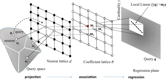
4.2.3 Coefficient output lattice
In this output lattice, if the local associative function is varying considerably around a point, a piece-wise constant approximation may require many units. In this case, we refer to the estimation of the local linear regression coefficients
mj = [mj0, mj1, . . . , mj2d] ∈ R2d+1, which are associ-ated with each query prototypewj. That is the cardinality y is approximated by a linear combination of the query dimensions q = [q1, . . . , q2d], while m is the (2d +1) -dimensional vector of the linear coefficients, withm0being the intercept in the R2d ×N space. The mj coefficients reside on a coefficient lattice O such that the j-th index of wj refers to thej-th regression plane governed by the regressionmjq. This defines a local regression plane over the query and cardinality space, defined by those queries that are projected on the query prototypewj. Hence, a point
mjin the coefficient lattice corresponds to the parameter of thelocal linear regression function:
fj(q)=mjq,q∈R2d :j =arg min
i∈[M]q−wi2. (9) Fig. 2 Cardinality lattice-based
prediction: Projection-association-local prediction: Simultaneous UCL and HCL over latticesLandC
wj q
wi wk
Neuron lattice Cardinality lattice
Query space query
neuron
Kernel regression
Figure3shows the idea of the coefficient lattice. In the case of input latticeLand output latticeO, the parameter set for modelMisα=({wj},{mj}), j=1, . . . , M.
4.3 Learning methodology 4.3.1 Overview
Consider the presence of a (random) training pair (q, y). The following steps demonstrate the methodology of exploiting such training pair for estimating the points on the: neuron, cardinality and regression lattices.
Projection The queryqfrom the training pair(q, y)is pro-jected onto its (winner) closest neuron wj ∈ L from the neuron lattice. Certain neurons, including the winnerwj, are then adapted to this occurrence. In this step, we have to define the update rulewifor the neurons in the neuron lattice.
Association Simultaneously, the actual cardinalityy from the training pair(q, y) is utilized to update certain points from the cardinality and regression lattices. Specifically, the corresponding prototypeyj ∈C, i.e., this is associated with the winner query neuronwj, and the corresponding regres-sion coefficientmj ∈ O are updated based ony and the query q (in the latter case) governed by feedback update rules. Such rules derive from the stochastic negative partial derivative (introduced later).
Prediction The modelMafter locating the winner neuron
wjbased on the input lattice, predicts the cardinalityyˆusing Kernel regression over (i) the local associative functions in theClattice, and (ii) the local linear regression functions in theOlattice.
Feedback The prediction resultyˆfeeds theCandOlattices for updating the cardinality prototypes and the regression coefficients, respectively.
4.4 The predictive learning algorithm
We adopt SOM for UCL since based on topology preserva-tion we can claim that:if queriesqandqare similar due to being projected onto the same neuronwjofL, then their
images through the local associative and local regression functionsfj(q)andfj(q)on cardinality latticeCand
coef-ficient lattice O, respectively, are likely to be similar, too. This argument cannot be claimed by any other UCL method (e.g.,k-means or fuzzyc-means clustering), which does not guarantee topological ordering of quantization vectors.
At this point, we can define the cardinality prediction function yˆ = f (q, α) based on the local associative and regression functions, and in the sequel, report on the loss functionL(y,y)ˆ . Consider two range queriesq,q normal-ized firstly in[0,1]2d (only for simplicity in our analysis). Let the winner neuron wj ∈ L and its corresponding (i) local associative functionfj(q), i.e., cardinality prototype yj ∈ Cand (ii) local linear regression functionfj(q), i.e., regression coefficientmj ∈Oto a random queryq.
The cardinality predictionf is not only based onfj(q), but also on the contribution of the neighboringfi(q)defined by the topographical neighborhood of winner wj. This is achieved by a kernel functionK(ri−rj2)over the nor-malized location vectors ri and rj (i.e., ri,rj ≤ 1) of the associated neurons wi and wj in the input lattice
L, respectively. That is,yˆ = f (q, α) is produced by the (Nadaraya-Watson) Kernel regression model:
ˆ y=f (q, α)= M i=1K(ri−rj)fi(q) M i=1K(ri−rj) (10) withj = arg minwi∈Lq−wi2. In this paper, we utilize
the kernelK(x)=0.75·
1−(x−0.5)2·I (|x−12| ≤), which is the Epanechnikov kernel function shifted to 0.5 and scaled by 0 < 0.5. Obviously, any other ker-nel functions can be also adopted e.g., uniform, triangular, quadratic, with Epanechnikov being most commonly used Fig. 3 Coefficient lattice-based
prediction: Projection-association-linear regression: Simultaneous UCL and HCL over latticesLandO
wj
q
wi
wk
Neuron lattice Coefficient lattice Query space query neuron mk mi Query q Cardinality y mj Local Linear fj(q) =mjqT Regression plane
kernel for regression. Topographically close neurons w.r.t. location vectors also imply close neurons w.r.t. Euclidean distance. However, the adoption of a Kernel function over the distance of neurons inR2dcould assume query compo-nents to be isotropically Gaussian, which is not a general case whendis relatively large. The predicted cardinalityyˆ is estimated by a kernel smoothing of those cardinality pro-totypes and linear regression coefficients, whose associated neurons are topographically close (w.r.t. ) to the winner neuron.
Given actualyand predictedyˆin (10), we then adopt the loss functions:
L1(y,y)ˆ = |y− ˆy|andL2(y,y)ˆ =(y− ˆy)2 (11) since there are widely used for evaluating the prediction error in cardinality prediction as in [11,15,27].
We can now provide the (on-line) learning phase of the modelM given a sequence of pattern (training) pairs (q(1), y(1)), (q(2), y(2)), . . .Query patternsq(t)are used for quantizing the query space (over L) and cardinalities y(t)are used for learning theq → y association (overC andO). Upon the presence of a pattern pair(q(t), y(t))the winnerwj(t)∈Lis determined by
j =arg min
wi∈L
q(t)−wi(t). (12)
After the projection of q to winner wj, the model M updates in an incremental manner the winner and all its neighbors of latticeLsuch that they approach the query pat-ternqwith a magnitude ofβ(t )h(i, j;t). In the same time, the actual cardinalityyis used for updating the correspond-ing: (i)yj ∈ C along with all prototypesyi ∈ C and (ii)
mj ∈ O along with all coefficients mi ∈ O associated with the neighbors of winner neuronwj. Notably, the update rules for eachyi andmiare governed by the loss function L(y,y)ˆ we aim to minimize, havingyˆdefined in (10).
In the case of the neuron-cardinality lattices for cardi-nality prediction, the model M estimates the parameter α = ({wi},{yi})Mi=1by minimizing the objective function
J1in (13) J1({wi},{yi})= 1 2 Ww i∈L h(i, j )wi−q22dp(W) + Yy i∈C h(i, j )|y− ˆy|dp(Y) (13) being taken over an infinite sequence of W = {q(1),
q(2), . . .} and corresponding Y = {y(1), y(2), . . .} and p(W),p(Y)is the pdf ofWandY, respectively, with
ˆ y= M i=1K(ri−rj)yi M i=1K(ri−rj) (14)
andj = arg minwi∈Lq−wi2. The factor
1
2 is for math-ematical convenience. Here, we utilize theL1in (11) loss function, since the cardinality prototypes are local scalar constant values within each query sub-space.
In the case of the neuron-regression lattices for cardi-nality prediction, the model M estimates the parameter α = ({wi},{mi})Mi=1by minimizing the objective function
J2in (15) J2({wi},{mi})= 1 2 Ww i∈L h(i, j )wi−q22dp(W) +1 2 Umi∈Oh(i, j )(y− ˆy) 2 dp(U) (15)
wherep(U)is the pdf ofm, withj =arg minwi∈Lq−wi2
and ˆ y= M i=1K(ri−rj)miq M i=1K(ri−rj) . (16)
Here, we utilize theL2 in (11) loss function, since we estimate the local linear regression coefficients within each query sub-space based on the ordinary least squares method.
Theorem 1 Given a training pair(q(t), y(t)), the model
Mconverges to the optimal parameterα, which minimizes the risk functionJ1(α)in(13)with respect to loss function
L1(y,y)ˆ = |y− ˆy|andyˆis defined in(14), if neuronwi(t)∈
Land its associated prototypeyi(t)∈Care updated as: wi(t)=β(t )h(i, j;t) (q(t)−wi(t)) (17) yi(t)=β(t ) M k=1 h(k, j;t)MK(ri−rj) k=1K(rk−rj) ×sgny(t)− ˆy(t) (18)
where sgn(·)is the signum function,β(t )is the learning rate andh(i, j;t)is the neighborhood function,jis the index of the winner neuronwj(t)of pattern queryq(t)and predicted
ˆ
y(t)is determined by(14).
The proof of Theorem 1 is provided in [5]; we present it here for self-contained reasons.
Proof We derive the analysis of convergence corresponding to latticesLandC. We verify whether the quantization error w−q22 and lossL1(y,y)ˆ = |y− ˆy| actually decreases as the learning phase proceeds, converging eventually to a stable state.
The convergence is evaluated through the average expected loss J1 in (13) being taken over an infinite sequence ofW= {q(1),q(2), . . .}and correspondingY = {y(1), y(2), . . .}andp(W),p(Y)is the pdf ofW andY, respectively. Since both pdfs are unknown and sequences
Y and W are actually finite we use the Robbins-Monro (RM) stochastic approximation forJ1minimization to find an optimal value for each wi, yi, i = 1, . . . , M. Based on RM the stochastic sample J1(t) of J1 is J1(t) = 1 2 wi∈Lh(i, j;t)wi(t)−q(t) 2 2+ yi∈Ch(i, j;t)|y(t)− ˆ
y(t)|. TheJ1(t)has to decrease at each new pattern att by descending in the direction of its (partial) negative gradient. Hence, the SGD rule for eachwiiswi(t)= −12β(t )∂J∂w1(t)
i(t)
and foryi isyi(t) = −β(t )∂y∂J1i(t)(t), where β(t ) satisfies
∞
t=0β(t )= ∞and
∞
t=0β2(t) <∞[21]. From the par-tial derivatives ofJ1(t)we obtain the update rules (17) and (18) for parameter setα.
Remark 1 Note that the update rule (18) for prototypes yi(t)involves the current predictiony(t)ˆ of the model dur-ing the t-th training pair in the learning phase. Naturally we update each yi(t) in an on-line supervised regression fashion, in which we take the predictiony(t)ˆ in (14) as feed-back. From (18) we observe that neighboryi(t)ofyj(t)is adapted by its relative contribution provided by the kernel function, which is rational sinceyi(t)contributes with the same magnitude to the cardinality prediction. Ify(t) >y(t)ˆ , thenyi(t)increases linearly with its contribution to predic-tion approaching the actualy(t). On the other hand, i.e., y(t) < y(t)ˆ ,yi(t)decreases to move away fromy(t)ˆ and approachesy(t). When the current prediction error is zero, i.e.,L(y(t),y(t))ˆ = |y(t)− ˆy(t)| = 0, there is no update on the cardinality prototypes. Neuronwi(t)moves toward pattern queryq(t)to follow the trend. Obviously, the more similar a pattern queryqand a neuronwi are, the lesswi gets updated.
Theorem 2 refers to the convergence of a neuron wi to the local expectation query representative, i.e.,centroid E[q|Qi]in the input sub-spaceQi.
Theorem 2 IfE[q|Qi]is the local expectation query of the
subspaceQi and prototypewi is the subspace
representa-tive,P (wi=E[q|Qi])=1at equilibrium.
Proof The update rule for a neuronwibased on Theorem 1 iswi∝(q−wi). Let thei-th neuronwireach equilibrium: wi = 0, which holds with probability 1. By taking the expectation of both sides we obtain
0= E[wi] =E[(q−wi)] = Qi (q−wi)p(q)dq = Qi qp(q)dq−wi Qi p(q)dq.
This indicates that wi is constant with probability 1, and then by solving E[wi] = 0, the wi equals the centroid
E[q|Qi].
If is selected such that K(ri −rj) = 0, i = j, then we obtain yj ∼ sgn(y −yj)in which only yj of the winnerwj is updated, given that there is no significant impact from other neighboring neurons after convergence, i.e.,Mk=1h(k, j ) t→∞= h(j, j ) ∼= 1. We then provide the following theorem:
Theorem 3 If y˜j is the median of the partition Yj
corre-sponding to the image of query sub-spaceQj of winnerwj
thenP (yj = ˜yj)=1at equilibrium.
The proof of Theorem 3 is provided in [5]; we present it here for self-contained reasons.
Proof Let yj correspond to wj and assume the image of
Qj ⊂ R2d to subspaceYj ⊂ Nvia the y = f (q). The mediany˜j ofYj satisfiesP (y ≥ ˜yj)=P (y ≤ ˜yj) = 12. Suppose that yj has reached equilibrium, i.e., yj = 0, which holds with probability 1. By taking the expectations of both sides and replacingyjwith the update rule sgn(y− yj): E[yj] = Yj sgn(y−yj)p(y)dy =P (y≥yj) Yj p(y)dy−P (y < yj) Yj p(y)dy =2P (y≥yj)−1.
Sinceyj = 0 thusyj is constant, thenP (y ≥ yj) = 12, which denotes thatyj converges to the median ofYj.
Theorem 4 Given a training pair(q(t), y(t)), the model
Mconverges to the optimal parameterα, which minimizes the risk functionJ2(α)in(15)with respect to loss function
L2(y,y)ˆ = (y − ˆy)2 and yˆ is defined in (16), if neuron
wi(t)∈ Land its associated linear regression coefficients
mi(t)∈Oare updated as:
wi(t)= β(t )h(i, j;t) (q(t)−wi(t)) (19) mi(t)= β(t ) M k=1 h(k, j;t)MK(ri−rj) k=1K(rk−rj) ×y(t)− ˆy(t)[1;q(t)] (20)
whereβ(t )is the learning rate and h(i, j;t)is the neigh-borhood function,j is the index of the winner neuronwj(t)
of pattern queryq(t)and predictedy(t)ˆ is determined by
(16).
Proof As in the proof of the Theorem 1, the conver-gence is evaluated through the average expected loss J2 in (13) being taken over an infinite sequence of W = {q(1),q(2), . . .}and corresponding Y = {y(1), y(2), . . .} and p(W). We rest on RM stochastic approximation
for J2 minimization to find an optimal value for each
wi, mi, i = 1, . . . , M. The stochastic sample J2(t) of J2 is J2(t) = 12wi∈Lh(i, j;t)wi(t)− q(t) 2 2 + 1 2
mi∈Oh(i, j;t)(y(t)− ˆy(t))
2. Hence, the SGD rule for eachwiiswi(t)= −12β(t )∂∂Jw2i(t)(t)and formiismi(t)= −1 2β(t ) ∂J2(t) ∂mi(t), where β(t ) satisfies ∞ t=0β(t ) = ∞ and ∞
t=0β2(t) < ∞ [21]. From the partial derivatives of
J2(t)we obtain the update rules (19) and (20) for parameter setα.
Remark 2 As seen in (20), when determining the positions of regression coefficients, supervised (prediction) error is not only taken into account, but also the input q and the impact ofallneurons (reflected by their neighborhood func-tions h(k;j ) are taken into consideration. Through this coupled training of the regression coefficients and neurons positions, query and regression representatives are placed in the input and output space, respectively, in such a way so as to minimize the loss functionL2.
Remark 3 Let us assume again that an is selected such thatK(ri−rj) = 0, i = j. Given that both neurons and regression coefficients converge from Theorem 4, then, we obtain the update rule:mj ∼(y−mjq)q, given that there is no significant impact from other neighboring neu-rons after convergence, i.e.,Mk=1h(k, j ) t→∞= h(j, j ) ∼= 1; here, for mathematical convenience, we absorbed the ’intercept’ constant of the local regression plane by adding a constant dimension of one to q. Evidently, this corre-sponds to the stochastic update rule for the multivariate linear regression utilizing the ordinary least squares method. The learning phase of model Mis described in Algo-rithm 1. The input is the training set of pairsQ= {(q, y)}, 2-dim. latticesLandC (orO) withM entries, and a stop-ping thresholdθ > 0. The algorithm processes successive random pattern pairs until a termination criterionTt ≤θ.Tt is the 1-norm between successive estimates of neurons and cardinality prototypes: Tt = M i=1 (wi(t)−wi(t−1)1+ |yi(t)−yi(t−1)|) , (21) or regression prototypes, Tt = M i=1 (wi(t)−wi(t−1)1+ mi(t)−mi(t−1)1) , (22) withwi1=2kd=1|wik|andmi1=2kd=+11|mik|. The output is parameter setα.
4.5 Set cardinality prediction
Once the parameter set α is trained (for both output lat-tice variants), and thus no more updates are realized on neurons, cardinality prototypes and local regression coeffi-cients, we predict the cardinalityyˆgiven a random queryq
as defined in (14) and (16). That is, we proceed with answer set cardinality estimation without executing the incoming queryq.
Firstly, the queryqis projected onto the neuron latticeL and its winnerwj is obtained. In the case of the cardinality latticeC, the corresponding cardinality prototypeyj is the associated constant of the query sub-spaceQj. In the case of the regression latticeO, the local regression coefficient
mj is obtained. The predictedCOUNTvalue isyˆ calculated by the Kernel regression over the region around the images fi(q) = yi in lattice C and fi(q) = miq in lattice O, respectively, such thatK(ri−rj) >0, fori=1, . . . , M.
4.6 Computational complexity
During the learning phase of the model M, we require to (i) find the closest (winner) neuron over the neuron latticeL and then (ii) update allMprototypes in both input and out-put lattices based on the neighborhood weighth(i, j ),∀i. This requires O(dM)space and O(dM)for the updates. Since prototypes are updated during learning, the learning
phase requiresO(d/θ )[10] iterations to getTt ≤ θ. After learning, we obtain cardinality prediction in O(dlogM) by applying an one-nearest neighbor search for the win-ner using a 2d-dim. tree structure over the neurons in L. After locating the winner, then we just retrieve those neigh-boring neurons (constant number) which are determined by the Kernel neighboring functionK. In the case of updates, adaptation given a pair requires alsoO(dlogM) time for searching for the winner. Hence, our proposed parametric model, after training, can provide prediction inO(dlogM), which is independent of the size of the data|B|and the train-ing set |Q|, thus, being capable for scaling out predictive analytics tasks.
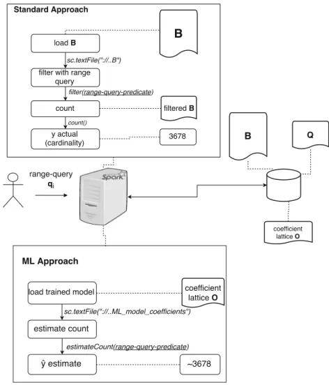
5 Implementation in Spark
We have implemented our model in the Spark system [32]. The reason behind this implementation is to explore how such models can be incorporated into Big Data Engines. In addition, we examine how much faster and how close our cardinality estimations are, compared with the result obtained from the built-in COUNT method provided by these engines. This section covers the basic concepts behind Spark [32] (currently a popular Big Data engine) and an overview of how we developed and incorporated our machine learning model into Spark.
5.1 Overview of Spark
The Resilient Distributed Datasets (RDDs) lie in the foun-dation of Spark. RDDs are fault-tolerant distributed data structures that allow users to save intermediate results in main memory. This means that, RDDs can be easily recov-ered once something goes wrong and that they can be easily distributed in a cluster environment to improve efficiency. Their recovery is relied on thelineage graph produced by Spark. A lineage graph is a Directed-Acyclic Graph that is used to record all of the changes made to a dataset. Hence, once something goes wrong it can be easily re-computed using the steps recorded. In addition, through this func-tionality, the users can control the number of partitions to optimize the data placement and, also, offer a rich set of operations [32]. The set of operations can be divided into
transformationsandactionswhich are described as follows:
5.1.1 Transformations in Spark
The RDDs are created by loading data files from permanent storage or by using transformations on loaded data. These transformations can change the loaded data through oper-ations such asfilter andmap. A comprehensive list of the
available transformations can be found at Spark’s website.2 It is worth noting that transformations are not applied imme-diately. Instead, Spark uses a lineage graph and pipelines successive transformations to the original dataset once an
actionis called [32].
5.1.2 Actions in Spark
Spark contains a type of methods calledactions. These oper-ations return a value to the application or export data into storage [32]. Example of those types of actions are: 1. COUNT, which refers to theexactcardinality of a given
query and corresponds to our ground truth for assessing the cardinality predictability of our model;
2. COLLECT, which returns a list of elements given a query;
3. SAVE, which stores the RDD into a permanent storage, e.g., HDFS or a local file system.
5.2 Machine learning model implementation
For UCL (Task 1), we implement the online SOM algorithm with M neurons. We make use of the neurons input lat-tice conceptLdescribed in Section4.2.1and we implement our UCL approach to partition the query space as described in Section 3.1.1. The neuron input lattice L contains all of our neurons and the winner is determined and updated as in (1) making use of Stochastic-Gradient descent. For HCL (Task 2), we implement the supervised linear regres-sion model making use of the coefficient output latticeO described in Section4.2.3, in which the coefficientsmj = [mj0, mj1, . . . , mj2d] ∈ R2d+1 are associated with each query prototypewj ∈L. We then generate our predictions using Kernel regression in (16).
5.3 Range queries workload
In our implementation and experiments we dealt with multi-dimensional queries corresponding to a 2-multi-dimensional data space (d=2). The two boundary vectors area= [a1, a2] andb= [b1, b2], ai≤bi, ai, bi∈R. Hence, in the exper-iments, a range queryqis represented by a 4-dimensional row vectorq= [a1, b1, a2, b2]. We further adjust this repre-sentation to ease up the process of generating our query set
Q. In this context, our resulting queries are of the formq=
[c1, c2, l]withcenterci = ai+2bi, andvolumel =bi−ai, i=1, . . . , d. Through this representation, each queryqis a hyper-cube.