Optimised Geographies for Data Reporting:

Optimised Geographies for

Data Reporting:

Zone design tools for census output geographies

Statistics New Zealand Working Paper No 09–01

Disclaimer

The Statistics New Zealand Working Paper series is a collection of occasional papers on a variety of statistical topics written by researchers working for Statistics New Zealand. Papers produced in this series represent the views of the authors, and do not imply commitment by Statistics NZ to adopt any findings, methodologies, or recommendations. Any data analysis was carried out under

the security and confidentiality provisions of the Statistics Act 1975.

Liability statement

Statistics New Zealand gives no warranty that the information or data supplied in this paper is error free. All care and diligence has been used, however, in processing, analysing and extracting information. Statistics New Zealand will not be liable for any loss or damage suffered by customers

consequent upon the use directly, or indirectly, of the information in this paper. Reproduction of material

Any table or other material in this paper may be reproduced and published, provided that it does not purport to be published under government authority and that acknowledgement is made of

this source.

Citation

Martin Ralphs and Lyndon Ang (2009). Optimised geographies for data reporting: zone design tools for Census output geographies (Statistics New Zealand Working Paper No 09–01).

Wellington: Statistics New Zealand

Published in December 2009 by Statistics New Zealand

Tatauranga Aotearoa P O Box 2922 Wellington, New Zealand

info@stats.govt.nz www.stats.govt.nz

Contents iii

List of tables and figures ... iv

Acknowledgements... vi

Abstract vii 1 Introduction ... 1

1.1 The Census of Population and Dwellings and small area geographies ... 1

1.2 Naming conventions and terms for geographical areas ... 2

2 Literature review ... 3

2.1 Census output geographies ... 3

2.2 The zone design problem in the literature ... 4

2.2.1 An algorithm for automatic zone design ... 5

2.3 Experience at the Office for National Statistics, United Kingdom ... 9

3 Software tools for automatic zone design ... 11

3.1 AZTool ... 11

3.2 GIS tools for data preparation ... 12

3.3 Hardware and software configuration used in the project ... 12

4 Datasets used in the evaluation ... 13

5 Setting up and calibrating the zone design toolkit ... 15

5.1 Exploring the impact of alternative contiguity options for meshblocks ... 15

5.2 Optimal number of AZTool iterations ... 18

5.3 Use of the shape compactness option... 20

5.4 Use of the homogeneity option ... 21

5.4.1 Evaluating homogeneity ... 22

5.5 Use of the simulated annealing option ... 26

5.6 Optimising all of New Zealand versus a single region ... 27

6 Zone design for census geographies: area units ... 30

6.1 Simulation results ... 31

6.1.1 Ability to meet minimum population size criterion; using population size as the population constraint... 31

6.1.2 Ability to meet minimum population size criterion; using household size as the population constraint... 32

6.1.3 Comparison with the 2006 area unit geography ... 34

7 Zone design for census geographies: meshblocks ... 37

7.1 Simulation results ... 38

7.1.1 Ability to meet population and household size criteria when using the population size constraint ... 38

7.1.2 Ability to meet population and household criteria when using the household size constraint ... 40

7.1.3 Shape compactness of new OA1 zones ... 40

7.1.4 Comparison with the 2006 meshblock geography ... 41

7.1.5 Constraining AZT OA1 zones to fit within AZT OA2 zones ... 43

8.1.1 Population thresholds and distributions ... 45

8.1.2 Shape compactness ... 45

8.1.3 Homogeneity ... 46

8.1.4 Nesting within larger geographical units ... 46

8.1.5 Algorithm performance ... 46

8.1.6 ArcGIS toolkit performance ... 47

8.2 Points to consider if the methodology is implemented ... 47

8.3 Suggestions for further research ... 48

References ... 49

Tables by section 1 Introduction

1.1 Standard geographical hierarchy as published in the 2006 Census ... 1

5 Setting up and calibrating the zone design toolkit 5.1 PWVar for dwelling type categories ... 23

5. 2 PWVar for Selected Person Characteristics ... 23

5.3 Comparing PWVar values for area units and output zones built with different sets of constraints ... 25

6 Zone design for census geographies: area units 6.1 Attributes of 2006 area unit (AU) geography ... 30

6.2 Population and household size targets ... 31

7 Zone design for census geographies: meshblocks 7.1 Results from AZT runs – constrained meshblocks ... 43

Figures by section 2 Literature review 2.1 Step 0 of automatic zoning procedure (AZP) algorithm ... 6

2.2 Illustration of step 1 of the AZP algorithm ... 6

2.3 Example of outcome from steps 2 and 3 ... 7

2.4 Example of completed steps 1 to 5 ... 8

2.5 Example of Step 7 ... 8

4 Datasets used in the evaluation 4.1 An example of single point contiguity ... 13

5 Setting up and calibrating the zone design toolkit 5.1 AZT output zones for part of Wellington, 100-metre minimum contiguity... 16

5.2 P2A values for 100m contiguities with minimum area condition, Wellington city territorial authority... 17

5.3 AZT output geography for part of Wellington region ... 17

5.4 Isolated meshblocks within the AZT output geography ... 18

5.5 Minimum target population objective function values ... 19

5.6 Shape compactness objective function values... 20

5.7 Shape and population measures after 15 iterations... 21

5.8 PWVar increase – dwelling type ... 24

5.9 PWVar increase – person characteristics ... 24

5.11 Distribution of minimum population sizes, Wellington city territorial authority ... 28

5.12 Distribution of mean population sizes, Wellington city territorial authority ... 28

6 Zone design for census geographies: area units 6.1 2006 area unit population distribution ... 30

6.2 Distribution of population size minimums and means ... 32

6.3 Distribution of household size minimums and means ... 32

6.4 Compactness distributions – area units versus AZT OA2 output zones ... 33

6.5 AZT OA2 output geography in Wellington city territorial authority ... 34

6.6 Empirical density function for area units compared with equivalent distributions for 30 sets of AZT OA2 zones ... 35

6.7 Household size distribution – 2006 area units versus AZT OA2 zones ... 35

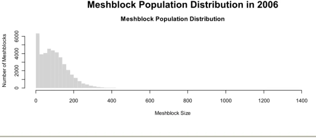
7 Zone design for census geographies: meshblocks 7.1 Meshblock population distribution in 2006 ... 37

7.2 Population and shape compactness measures after 15 iterations across 30 AZT simulation runs ... 38

7.3 Number of output tracts which do not meet minimum constraints ... 39

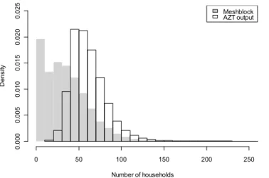
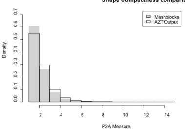
7.4 Distribution of household sizes – meshblocks versus AZT output ... 40

7.5 P2A distributions – meshblocks versus AZT OA1 geography ... 41

7.6 Population size – original meshblock geography versus AZT OA1 zones ... 42

The authors would like to thank Professor David Martin and Ms Sam Cockings of the Department of Geography, University of Southampton, United Kingdom, for permission to utilise and to modify the AZTool computer program for use in this project. AZTool is copyright © 2008 David Martin.

This paper explores methods that might be used to construct new geographies for data reporting that are in some sense optimised. The objective of the paper is to evaluate an automatic method for generating robust statistical output zones that fulfil pre-specified optimal characteristics such as compactness of shape, minimum population size, standard mean population size, and constrained nesting within larger areas. We apply a spatially aware method from the computational geography literature to design new reporting geographies, using 2006 Census data as the main input. We compare the new geographies with existing, official geographies, addressing two criteria: firstly, the stability and performance of the optimisation algorithm, the impact of different control parameters, and the robustness of the solutions generated; and secondly, the statistical quality of automatically generated geographies in terms of population distributions and minima, shape compactness, and internal homogeneity.

We find that our new geographies substantially out-perform the current geographies across almost all of our optimisation criteria. The algorithm that we use is stable, and is able to repeatedly generate high-quality solutions in a timely manner. We conclude that the ArcGIS / AZTool toolkit developed here would form the basis of a viable workflow for the automatic production of optimal geographical areas.

Key words

Computational geography, zone design, supervised regionalisation methods, combinatorial optimisation, automatic zoning procedure, optimal geographical areas.

This paper considers the use of spatially aware, stochastic methods drawn from the field of computational geography for the optimal generation of census output geographies at the New Zealand area unit and meshblock levels. It describes the results of a series of experiments to design new output geographies with optimal properties, and compares the resulting geographical output units with the existing 2006 Census output

geographies. 2006 Census data are used as the main basis for comparison.

We note at the outset that the work described here is experimental and is concerned primarily with a technical analysis covering proof of concept. While the methods and techniques we describe show considerable promise, the redrawing of Statistics New Zealand’s small area output geographies is a major undertaking that will require

consultation with stakeholders, careful planning, and significant resource. This is a matter for future consideration. The paper does not address the policy or resource implications of implementing the methods we describe.

1.1

The Census of Population and Dwellings and

small area geographies

The New Zealand Census of Population and Dwellings is conducted once every five years. It collects information from every individual within the nation, and provides an official count of population and dwellings at a point in time. The information collected provides a snapshot of various aspects of New Zealanders' lives, and includes data on the composition of the population, what types of houses people live in, what they earn, and what industries they work in (Statistics New Zealand website, 2006).

Census data is disseminated at several geographical levels; in fact, because information is collected from each individual in the population, it is possible to publish relatively accurate census statistics at fine levels of geography.

Table 1.1

Standard Geographical Hierarchy as Published in the 2006 Census

Meshblocks 41,362 87

Area units 1,909 2,100

Territorial authorities 72 55,100

Regional councils 16 251,000

Concern has been raised about the relevance and utility of the finer-level meshblock and area unit geographies for users of census data. Area units were created over 20 years ago and no longer adequately delineate real communities on the ground or meet the needs of key user groups in parts of New Zealand. Meshblocks are designed primarily for data collection rather than output. In practice, this means that they are not necessarily useful for output purposes because the fact that their boundaries are drawn

to aid data collection may mean that they cross-cut important patterns of local socio-economic variation on the ground. The wide ranging population sizes within both area units and meshblocks further contribute to problems with confidentiality in census data. In some cases, this issue limits the amount of data that can be made available.

One way to address these concerns would be to generate new, output-focused fine-level geographies. Such output geographies should be in some sense optimal, in order to try and overcome the problems present in the existing hierarchy. Since the

delineation of geographic units that fulfil particular criteria is a labour-intensive manual process, new area geographies would also, ideally, be constructed in an automated manner.

The rest of the paper is divided into 6 sections. Section 2 introduces the problem and reviews the methods that other researchers have used to address these issues. Sections 3 through to 7 introduce the software tools that we have used and present some results for 2006 area unit and meshblock geographies. Section 8 draws conclusions based on our findings.

1.2

Naming conventions and terms for

geographical areas

Since New Zealand has an official geographical reporting unit called the ‘area unit’, we use the following terms when referring generically to area-based geographical reporting units in this paper:

• ’Zone’ refers generically to any geographical area.

• ’Output geography’ or ‘geography’ refers generically to a predefined

collection of geographical areas. Three examples of output geographies used in New Zealand are ‘area unit’, ‘meshblock’, and ‘territorial authority’.

• ‘Reporting zones’ and ‘output zones’ refer generically to groups of

This review begins with a description of the issues that need to be considered when designing appropriate census output geographies, and in particular the criteria required for an effective output geography. We then discuss how the design of such geographies might be accomplished with a brief review of the research literature in this area. We conclude the review with a short description of the automatic zoning method that we have deployed and how it has been used to produce output geographies for the 2001 Census for England and Wales.

2.1

Census output geographies

Census geography describes the division of the country into geographical zones for census purposes. An appropriate census geography system should, first of all, facilitate the organisation and management of the census itself; secondly, it should facilitate the publication of small area statistics which meet users' needs (Martin, 2002). In other words, within the census geography system, we make a distinction between an ‘enumeration geography’ for collecting census data, and an ‘output geography’ for reporting census results. In practice, most countries use the same census geography for enumeration and dissemination at the smallest level (Alvanides, 2000). New Zealand is no exception, with the meshblock geography currently being used for both enumeration and dissemination purposes.

Unfortunately, the most appropriate census enumeration geography will most likely not be the most appropriate output geography. Census enumeration zones are operational units constructed for data collection purposes, and so will seldom adequately represent underlying socio-economic processes (Morphet, 1993). An additional concern is that the substantial amount of variation in population size that is typical of census

enumeration zones will lead to an increased risk of disclosure. Furthermore, these large variations in population sizes can result in non-comparable units for analysis (Cole, 1993). Census users themselves recognise this, and have expressed little support for the use of census collection areas as output zones (Rees, 1998).

An ideal census output geography should maximise the utility of published statistics for users, while at the same time limiting disclosure risk due to small population sizes. Martin's (1998a, 1998b) criteria for effective output geographies include the following:

• Standardising output zones by population size • Ensuring compactness of zone shape

• Maximising social homogeneity within zones

• Ensuring that output zones exceed a particular population size threshold.

The simultaneous optimisation of these competing criteria can pose a problem. Indeed, Alvanides (2000) states that the criteria as stated in the above form may not strictly be the best ones for census purposes. In order to obtain an appropriate solution for census output, the criteria can, and probably should be relaxed somewhat. Alvanides contends that we are simply looking to ensure that all output zones pass a certain minimum level of quality, as measured by the above four criteria. In other words, we desire that output zone population sizes lie within a certain threshold, and that they each exceed a certain

level of homogeneity and compactness. As Alvanides notes, "it is far more important to avoid the occasional straggling or spindly shaped output zone [than] it is to insist that all zones are approximately circular in shape, which is a highly unrealistic goal".

2.2

The zone design problem in the literature

There is an extensive literature relating to techniques for constructing aggregations of geographical areas that are in some sense optimal. The field is diverse and has been evolving for over thirty years. It spans a number of disciplines, including computational geography, and several aspects of operations research including graph theory,

combinatorial optimisation, and computational complexity (Raffensberger, 2008). A useful review is provided by Duque et al. (2007), who use the collective term

‘supervised regionalization methods’ to encompass the approaches and platforms used to tackle the problem. All of these methods attempt to aggregate a collection of input areas into a smaller number of spatially contiguous regions while optimising a set of aggregation criteria.

The zone design problem is difficult to solve computationally. The most basic approach would be to enumerate all possible area partitions that could be generated, and choose the one that best fits our optimal criteria. This is not feasible in practice, because the number of possible partitions is usually effectively infinite, and each solution has to be constrained geographically. Because of the complexity of the problem, most methods in the literature employ an heuristic approach to find solutions that are reasonably optimal. All of the solutions require neighbourhood contiguity information (in other words, to know which areas are next to which others) as a primary input.

The heuristic approaches employed include:

a) clustering algorithms which merge only contiguous areas b) starting from seed areas and adding neighbours

c) starting from a feasible initial solution and swapping zones in and out d) graph theoretic approaches.

(Duque et al, 2007).

While all of these methods may have application in the problem of census output area design, a key issue for Statistics NZ was the limited availability of robust tools to solve this class of problem. The zone design methodology adopted in this project utilises approach c), and is drawn from the field of computational geography. Our choice of this methodology above the others was driven by practical considerations:

• Method c) has seen successful prior use for a virtually identical problem in

the generation of census output geographies in the United Kingdom.

• A stable software package is already available to implement it through the

efforts of researchers at the University of Southampton, United Kingdom, without the need for a lengthy development exercise.

Statistics NZ has been experimenting with a graph theory approach to combinatorial optimisation alongside this project, in collaboration with the Department of Management at Canterbury University. This graph theory algorithm is being deployed in the design of enumeration areas with even workloads for the 2011 Census (Raffensberger, 2008). Although the graph theory approach might also be usable here, it was not feasible to

Optimised Geographies for Data Reporting by Martin Ralphs and Lyndon Ang

compare the two methods in this project because of timing and resource constraints. The other approaches noted by Duque et al may also have merit for our problem, but evaluating them is outside the scope of this paper because of the prohibitive resource cost of constructing new tools to carry out the procedures they describe.

2.2.1 An algorithm for automatic zone design

The zone design process involves the aggregation of N spatial zones into M bigger zones, where M is less than N, and where the M zones should be internally connected and contiguous (Openshaw and Rao, 1995). The aggregation procedure aims to find an optimal value for an objective function, which reflects the criteria that we are looking to achieve within the output zones. For example, objective functions may be constructed in order to obtain equal population size within each zone, or so that each zone exceeds a minimum population threshold. We can specify any criteria for an objective function to optimise. For designing census output zones, the criteria in section 3.1 form our starting point.

The algorithm deployed in this project is an implementation of Openshaw’s zone design algorithm (see Openshaw 1977, 1978). Zone design was proposed by Openshaw (1977) as a means of addressing the geographical partitioning and scale effects which together comprise the ‘modifiable areal unit problem’ (MAUP), a well-known issue in area-based analysis (see Openshaw (1977) for a full discussion). A brief outline of the problem is provided in appendix A for the interested reader.

Termed by Openshaw as the ‘automatic zoning procedure’ (AZP), the algorithm begins with an initial random aggregation of small areas into larger, candidate output zones. This initial zonal arrangement is then modified iteratively such that we optimise a given objective function. As mentioned before, this function will reflect the criteria (eg equal population size, homogeneity, or compactness) we require the output zones to achieve. The original AZP algorithm starts with a set of N input building block areas. Let us denote these a1 … aN. Given this input, the algorithm consists of the following steps:

Step 0: Create an initial random aggregation of the building blocks into M internally contiguous output zones z1, z2…zM, where M < N and each building block a is assigned to a single output zone. Calculate the value of the objective function for this starting aggregation. An example of such a starting configuration is shown in figure 2.1, where our building blocks have been aggregated into seven output zones:

Figure 2.1

Step 0 of Automatic Zoning Procedure (AZP) Algorithm

Example of a starting configuration of AZP

Step 1: Randomly select any zone zm from the initial random set. Now make a list of those building blocks which share a border with zm, but are not contained by it. We denote this list as B, and its members aB1 … aBn. In this example, zone z5 has been selected as zm and the building blocks which share a border with it (highlighted in dark grey in figure 2.2) become the first members of B.

Figure 2.2

Optimised Geographies for Data Reporting by Martin Ralphs and Lyndon Ang

Step 2: Randomly select and remove a single building block aBn from this list. For example, in figure 2.3, building block aB12 has been selected and is highlighted with a white surround.

Step 3: Identify the zone that building block aBn currently belongs to, denoted as zq. In figure 2.3 zone z7, which currently contains building block aB12, becomes zq.

Figure 2.3

Example of Outcome From Steps 2 and 3

Step 4: If the remaining building blocks in zq are contiguous then proceed to step 5. If they are not contiguous (ie removing this building block means that zq becomes fragmented), restore the building block to its original zone and return to step 2. In figure 2.3, removing aB12 from z7 does not fragment z7, so we can continue.

Step 5: Accept the move of building block aBn into candidate output zone zm, and calculate the new value of the objective function for this revised aggregation, see figure 2.4.

Figure 2.4

Example of Completed Steps 1 to 5

Step 6: If the new value of the objective function is an improvement on the previous value (found in step 0) then proceed to step 7. If not, restore the previous classification (returning aB12 back to z5 in our example) and return to step 2.

Step 7: The new value of the objective function is the new best value. Extend the list B by adding in building blocks that are outside zm but connected to aBn, which is now a member of zone zm. The new set of building block neighbours is highlighted in grey in figure 2.5. Notice that we now include all the neighbours of block aB12 as well. Figure 2.5

Example of Step 7

Optimised Geographies for Data Reporting by Martin Ralphs and Lyndon Ang

Step 8: When the list of bordering building blocks to zone zm is exhausted (that is, B is empty), then return to step 1.

Step 9: Repeat steps 1-8 until the algorithm converges. That is, the change in the objective function is less than a specified tolerance.

The original AZP is "a mildly steepest descent algorithm" (Openshaw and Rao, 1995, p429). It is performing a local search within the vicinity of a randomly selected zone, and makes changes to zone membership as soon as a better value for the objective function is found. We can compare this to a strictly steepest descent algorithm, which would try to identify the "best possible move between all possible pairs of areal units across all zones that provides the best value for the objective function" (Alvanides, 2000, p85).

One of the problems with the original AZP algorithm is that it can sometimes be trapped by local optima. Openshaw and Rao (1995) provide two variants of traditional AZP which help to alleviate this problem. In particular, the simulated annealing (SA) variant appears to improve the performance of AZP, although it does result in longer execution times; further examples can be found in Bowdry (1990) and Miller (1996). The SA method allows zone changes which actually result in a less optimal value of the objective function - this gives it a chance of moving out of situations where it might be stuck in a local sub-optimum. The probability of moving to a less optimal solution decreases as the number of iterations increase.

Finally, note that the number of output zones in the optimal solution is not

predetermined, but is decided by the algorithm based on the specified constraints and thresholds.

2.3 Experience at the Office for National Statistics,

United Kingdom

For the 2001 Census for England and Wales, the Office for National Statistics constructed a statistically optimised output geography for data reporting. New ‘output areas’ , built up from household-level postal address data, were created specifically for the publication of small-area census statistics. These output areas were different to the enumeration areas used for data collection, which had in previous censuses been used for both data collection and dissemination in England, Wales, and Northern Ireland. Scotland had developed a set of output areas for the 1991 Census outputs.

Openshaw's AZP algorithm was used to combine small geographical building blocks into larger zones. The effectiveness of the AZP algorithm for census output zone creation had previously been demonstrated by Openshaw and Rao (1995), and this concept was developed further by various parties, including Martin (1997; 1998b), Openshaw et al (1998), and Alvanides (2000).

The census zoning system was developed by the United Kingdom’s Office for National Statistics (ONS) in close collaboration with David Martin from Southampton University. It was designed to create zones above minimum population and household threshold sizes of 100 and 40 respectively, tightly grouped around a target household size of 125. The algorithm also attempted to create zones with a compact shape and with a degree of homogeneity in terms of housing tenure and type. Output areas were designed to be nested within ward and parish boundaries. Although there were some concerns as to

the resulting abstract nature of output area boundaries, the ONS believes that the solution obtained by their system was broadly seen as a success (ONS, 2002, p19). The approach was extended to create higher level geographical reporting units composed of groups of output areas and optimised using similar criteria for uniformity of population and household size. These higher level units, known as ‘super output areas’, have now replaced the administrative reporting zones that had been previously used for census dissemination as the main geographical hierarchy for census statistical outputs.

Further details on the automated creation of output areas for the 2001 Census for England and Wales can be found in Martin (2002).

In this section, we describe the zoning program and geographical information system (GIS) software tools we used in the project.

3.1

AZTool

There are no commercial solutions available for constructing output geographies using heuristic optimisation. However, Stan Openshaw and his team at the University of Leeds created the ZDES algorithm and toolkit in the late 1980s for tackling this problem. Further refinements to ZDES were carried out by Alvanides (1998), but development was restricted to UNIX software environments and FORTRAN coding.

AZTool (AZT) is a Windows application developed by David Martin and the GeoData Institute at the University of Southampton, United Kingdom, for generating optimal geographies using Openshaw’s AZP algorithm. It is written in Visual Basic. We are very grateful to David Martin and his team for allowing us to use AZTool in this research project. The version of AZTool deployed at Statistics NZ was modified by the authors in collaboration with Southampton University to allow for the processing of very large zonal datasets.

The program takes as input two datasets – the first dataset contains information on the contiguities between the building-block input zones, and the second contains

information relating to each zone. The user may specify various constraints that the algorithm needs to meet, including:

• minimum population threshold • target Population size

• shape compactness • output zone homogeneity.

In addition, the user may specify various options as to how AZT will operate. This includes how many iterations AZT will run for, whether donuts are allowed (that is, one output zone being completely enclosed by another), and whether AZP will be run using ‘simulated annealing’. A further option allows for the output zones to be wholly

contained within larger regions. New output zones generated from meshblocks can, for example, be constrained to nest within a territorial authority.

The AZT algorithm is a stochastic procedure, so each run will end up with a different output geography. The algorithm is therefore usually run over a number of iterations, each of which produces a candidate output geography, and the best result from those iterations is kept as the final output. More detailed information on the AZT algorithm can be found from the AZT program help file. The results contained within this document have all been produced using AZT. In all, several hundred different output geographies were created during the course of the project. It was encouraging to note that the results produced by AZT are very consistent across runs with similar input parameters.

The remainder of section 3 will discuss results from work conducted to refine the various AZT input parameters for creating effective output geographies.

3.2

GIS tools for data preparation

The AZTool package requires two input datasets: a file of contiguity information, which defines neighbourhood connectivity between building blocks, and a table of thematic data used to drive the optimisation engine. These text files follow a proprietary format based on outputs from Environmental Systems Research Institute’s Arc/INFO

Workstation software, a legacy of the development cycle of AZTool and ZDES. ArcINFO Workstation is not available at Statistics NZ. In order to use AZTool, a set of custom tools was built in ArcView 9.3 using the C#.NET development platform. These enable a user to construct AZTool input files, carry out some basic pre-processing tasks to improve the quality of AZTool outputs by limiting possible local neighbourhoods, and to take AZTool outputs and construct geographical datasets of optimal spatial units from them. The result is a toolbox that permits a complete workflow for optimal area

generation and can be installed alongside any ArcView 9.3 license. ArcGIS utilities for AZTool include:

• AZTool Exporter – allows the user to generate contiguity information and

export it. The tool includes various parameters, including the ability to restrict which areas count as contiguous.

• AZTool TractBuilder – takes AZTool output files and constructs tract

geographies from them. Can generate multiple output datasets from multiple tract files.

3.3

Hardware and software configuration used in

the project

All simulations in the project were conducted on a standard Statistics NZ desktop PC with a 2.66Ghz Intel Core2 Duo E6750 processor, 2GB of RAM, and a 250GB SATA300 Seagate Barracuda ES.2 7200rpm hard drive with 16MB cache. The PC was running Microsoft Windows XP SP2.

The project used 2006 meshblocks for New Zealand as the building blocks for creating new output geographies. The 2006 digital meshblock boundaries for New Zealand are readily available from the Statistics NZ website1_.

Meshblock boundaries were processed using the ArcGIS toolkit described in section 3.2 to produce a contiguities file containing information on which meshblocks were

neighbours. For an initial set of calibration runs, we included all meshblocks in the AZT optimisation, as well as all their respective contiguities. Results from these runs

prompted the removal of meshblocks that were not inside a territorial authority from the contiguities file. Additionally, single point contiguities (see figure 4.1 for an example) were not permitted in subsequent AZT runs.

Figure 4.1

An Example of Single Point Contiguity

Note: These two areas touch at a single shared point. They will be flagged as contiguous by ArcGIS unless programmed to discount this type of adjacency.

Data from the 2006 Census were used to create an intersection file containing attributes for each meshblock in the contiguities file. For each meshblock, the intersection file can contain such information as:

• Region ID of a larger geographical region that the meshblock belongs to –

this data can be used to restrict AZT processing to a single region, or to ensure that AZT produces output zones that are wholly contained within particular regions

• Population data – this can be the number of usual residents or households

within the meshblock

• Area – Area size of the meshblock

• Homogeneity information – this may include, for example, data on dwelling

type within each meshblock.

1

In the majority of AZT simulations conducted in this project, we constrained each output zone to nest within a territorial authority. We ran simulations using both usual residents and household population data as our population constraints. AZT’s homogeneity option was generally not used, except in section 5.7.

This section describes the set of calibration experiments we undertook to establish working parameters for AZTool before deployment. We considered the following issues:

• The impact of different ways of establishing local contiguity between

meshblocks on the performance of the zoning algorithm.

• The number of algorithm iterations required to obtain a useful solution and

the typical quality of the outcomes that resulted.

• The use of multiple optimisation criteria and the effect of including shape

compactness and homogeneity constraints as well as a population size limit.

5.1

Exploring the impact of alternative contiguity

options for meshblocks

A desirable outcome when designing output zones is that they have compact shapes. We measure shape compactness by comparing the squared perimeter with the area of each output zone. We call the resulting metric the P2A score. P2A is defined as:

P2A increases in value as the compactness of a shape decreases. The minimum (and most desirable) P2A value that can be achieved is 1, for a circle.

Using ArcGIS to pre-process the inputs for AZTool, we were able to control the definition of local adjacency between building blocks through the application of some simple threshold parameters. These included:

• The option to disallow single point contiguities.

• The option to disallow contiguities between areas whose shared border

length fell below a user-specified threshold.

• The option to turn off contiguity filtering if building blocks cover a smaller

area than a threshold value.

By removing point contiguities, we reduce the freedom with which AZT can form output zones. In particular, it was found that removing point contiguities serves to increase the shape compactness of AZT output zones.

We considered that putting in place a minimum threshold in terms of the length of the shared border between two building blocks might increase the level of compactness exhibited by output zones. To examine this, we produced two new sets of contiguity files with which to produce output geographies – one with a 50-metre minimum contiguity length and one with a 100-metre minimum contiguity length.

Our results indicate that when a minimum contiguity threshold is added, we do increase the shape compactness of AZT output zones. Additionally, the level of shape

compactness increases as the minimum contiguity length is increased. area perimeter s compactnes 2 4 1 π =

Care must be taken when incorporating a minimum contiguity threshold into the

contiguities file. Very small meshblocks may end up being isolated from their neighbours because they do not have any common boundary lengths which are long enough to meet the minimum threshold. These meshblocks would not be joined with any other meshblocks during the AZT optimisation process.

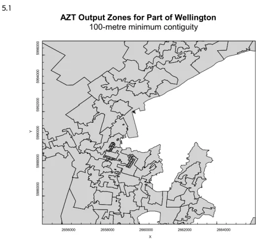
Figure 5.1 provides an example of this issue. This map contains a portion of the Wellington region, optimised in AZTool using the 100-metre minimum contiguity length when determining local adjacency. Around the centre of the map are a number of isolated meshblocks which have not been amalgamated into larger units. These ‘orphan’ meshblocks have boundaries that are uniformly shorter than the minimum contiguity length.

Figure 5.1

AZT Output Zones for Part of Wellington

100-metre minimum contiguity

In order to address this issue of isolated meshblocks, we can add a condition to bypass those meshblocks which are too small. In this case, input meshblocks that fall below a user-specified area size are not subject to the minimum shared border length filtering rule.

When using a 100-metre contiguity threshold, together with this minimum area condition, we successfully produce output zones which are fairly compact in shape. In figure 5.2 we have included the distribution of shape compactness values within the Wellington city territorial authority for one AZT run. The shape distribution for the original area unit geography is also included in light grey for comparison. While AZT does not generally produce as compact a shape distribution as the original area unit geography, we can see that there is a significant overlap between the two distributions.

2656000 2658000 2660000 2662000 2664000 5986000 5988000 5990000 5992000 5994000 5996000 X Y

Optimised Geographies for Data Reporting by Martin Ralphs and Lyndon Ang

Figure 5.2

P2A Values for 100m Contiguities With Minimum Area Condition

Wellington city territorial authority

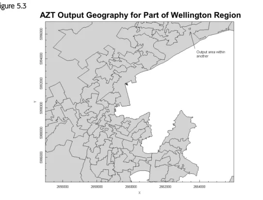
Figure 5.3 is a map containing the output zones from part of the Wellington region for one of the AZT runs. The general problem of isolated input meshblocks seems to have disappeared with the addition of the area condition. We can also see that the output tracts seem quite compact in shape. However, there is an isolated meshblock that was ignored by the AZT optimisation (in the top right hand corner). This suggests that some additional work still needs to be done to tweak the minimum contiguity and area thresholds so that isolated meshblocks do not occur.

Figure 5.3

AZT Output Geography for Part of Wellington Region

P2A Value D ensi ty 0 2 4 6 8 10 0.0 0.1 0.2 0.3 0.4 0.5 _{Area Units} Output Tracts

Another issue is illustrated in figure 5.4. The figure contains a portion of the output geography from the Auckland region, for one of the 100-metre minimum contiguity runs with the minimum area condition. Three meshblocks (shaded in dark grey in the figure) were not included in the AZT optimisation. These are on an offshore island, connected to the mainland by a narrow causeway. Even though these meshblocks are quite large and they exceed the minimum area threshold, the common boundary which links the left-most meshblock with the other meshblocks is most probably below the minimum contiguity threshold.

Figure 5.4

Isolated Meshblocks Within the AZT Output Geography

In general, the use of a minimum contiguity threshold aids in producing more compact AZT output zones. In doing this, one must be wary that meshblocks do not become isolated from their neighbours. The addition of a minimum area size condition, whereby the minimum contiguity threshold is only applied to areas which also exceed a

minimum area size, alleviates, but does not completely solve, this problem at present.

5.2

Optimal number of AZTool iterations

An initial set of 30 AZT calibration runs were conducted to examine the behaviour of the various objective functions as the algorithm progressed. This was done to ascertain how many iterations would generally be needed to result in a good solution. In each

calibration run, we executed 50 iterations of the AZTool algorithm and applied two objective functions: minimum target population and shape compactness. The 2006 Census meshblock geography was used as the input in all cases.

In Figure 5.5 we have plotted the behaviour of the minimum target population objective function as the number of iterations increases. The solid blue line represents the mean value, over the 30 runs, of this objective function at particular iterations.

The dashed grey lines are the minimum and maximum values of the target population objective function that were realised at a particular iteration, over the 30 runs.

Optimised Geographies for Data Reporting by Martin Ralphs and Lyndon Ang

The objective function decreases quite rapidly within the first 10 iterations, but by iteration 15 onwards we can see that the rate of improvement is uniformly very small.

Figure 5.5

Minimum Target Population Objective Function Values

Figure 5.6 shows how the shape compactness objective function changes as the number of iterations increase. From examination of figures 5.5 and 5.6, we see that there is a trade-off between the two objective functions – as one of them decreases, so the other increases. There is a larger change in the shape compactness objective function within the first 10 iterations. However, by about iteration 15 the rate of deterioration in shape compactness appears to become very small.

M ax/M in P op target value M ea n P o pta rg et va lue

Figure 5.6

Shape Compactness Objective Function Values

5.3

Use of the shape compactness option

The use of the shape compactness option introduces a shape objective function into the AZT optimisation process, and should facilitate the production of more compact output zones. The shape compactness constraint used by AZTool is perimeter squared divided by area, where more compact shapes will have a lower shape compactness value. This is a similar statistic to the P2A measure we defined in section 5.1.

In figure 5.7 we have plotted the target population and shape measure values for two sets of runs – one set using the shape constraint, and one set without the shape constraint. The objective function values are the final values at the end of 15 iterations. The light grey circles are the runs without the shape constraint, and the dark triangles are those with the shape constraint.

It is evident that the shape constraint makes a significant improvement to the shape measure. There is a clear separation between the group of AZTool runs with the shape constraint turned on, and the group without the shape constraint.

It was thought that with the shape constraint turned on, the target population measure would suffer as a result of the AZTool algorithm trying to find a balance between the shape and target population constraints. However, this was not the case. Even with the shape constraint turned on, the final population measure values are comparable to those obtained when the shape constraint is turned off. At the same time, the shape measure improves considerably.

Max/Min P2a target value Mean P2a target value

Optimised Geographies for Data Reporting by Martin Ralphs and Lyndon Ang

Figure 5.7

Shape and Population Measures After 15 Iterations

5.4

Use of the homogeneity option

The homogeneity option allows the user to create more homogenous output zones with respect to one or more specified homogeneity variables. The creation of more

homogenous output zones aims to fulfil the social homogeneity criterion specified in section 2.1.

Our examination of the homogeneity option made use of two sets of variables, for which data was obtained using 2006 Census meshblock-level data. These were:

1. Dwelling type, condensed into five categories (the ‘other’ category was ignored):

• ‘other private’ – Other private dwellings and occupied private dwellings not

further defined (NFD)

• ‘separate house’

• ‘joined private’ – two or more flats/houses/etc joined together • non-permanent

• ‘special dwelling’ – other non-private dwellings and occupied non-private

dwelling NFD institutions, and non-permanent special dwellings. 2. Three person-level characteristics:

• Mäori descent • disabled • unemployed.

These variables represent one possible set for measuring homogeneity. They were selected as a reasonable proxy for the type of information we might use when deciding

1.8e+08 2.0e+08 2.2e+08 2.4e+08 2.6e+08

350000 400000 450000 500000 550000 Population Measure P 2A S hape M easu re No Shape constraint Shape constraint

if areas are homogeneous, but other variables could be used. There may be better variables available and this may become clearer after consultation – for example, we may wish to differentiate between rural and urban areas.

AZT was run using two input datasets – firstly with all of New Zealand, and secondly using only the Auckland city territorial authority (TA). We ran AZT on the Auckland city territorial authority so that we could examine whether the change in homogeneity would be relatively greater in regions containing more small-sized areas. Our conjecture was that large numbers of small areas would provide the algorithm with lots more possible aggregation options, increasing flexibility and enhancing the quality of the solution.

5.4.1 Evaluating homogeneity

The measure that we used to evaluate the homogeneity of the output geographies produced by AZTool was the ‘population-weighted between-area variance’ of the output zones. This is a standard variance, weighted to take account of differences in the population size of zones across different geographical configurations. This statistic is henceforth abbreviated to PWVar.

PWVar is calculated over all the output tracts in a given output geography and produces a single value. For a given homogeneity variable x, higher values of PWVar correspond to higher between-area variances, and hence a lower within-area variance (and

correspondingly high internal homogeneity). For more homogenous areas, then, PWVar will be greater.

PWVar is calculated using the following formula:

2 1 1 ( ) A a( a ) a PWVar x N x x N = =

∑

where a is an individual area, x is the target variable in question,

x

Note that the local area mean is defined thus: 1 , a N i i a i a a x x N ∈ = =

∑

The global mean is defined as 1 1 , a N A i i a a i x x N ∈ = =

=

∑∑

local area means.

The PWVar values from the original meshblock and area unit geographies are the base from which we can compare the level of homogeneity resulting from our AZTool runs. The level of homogeneity for the meshblock geography is the best that we would be able to achieve, as we are forming our new output zones by aggregating these

meshblocks. We would like the level of homogeneity for the AZT output zone units to be greater than for the area unit geography.

In table 5.1 we have listed the PWVar for the meshblock and area unit geographies, using the dwelling type variable. PWVar was calculated for the Auckland city territorial authority as well as for all of New Zealand. Note that PWVar is higher (as expected) for the meshblock geography. PWVar is quite small in general; this is expected for real-world census areas. It tends to be higher in urban areas, probably because the variation of

Optimised Geographies for Data Reporting by Martin Ralphs and Lyndon Ang

homogeneity variables in the city is captured more effectively by the reporting zones (which tend to be small) than it is in more rural areas.

Table 5.1

PWVar for Dwelling Type Categories

Region of interest Other private Separate house Joined private Non permanent Special dwellings Meshblocks Auckland city 0.00099 0.00877 0.01468 0.00006 0.00003 All 0.00058 0.00748 0.00769 0.00024 0.00010 Area units Auckland city 0.00044 0.00469 0.00677 0.00005 0.00000 All 0.00016 0.00417 0.00373 0.00007 0.00002

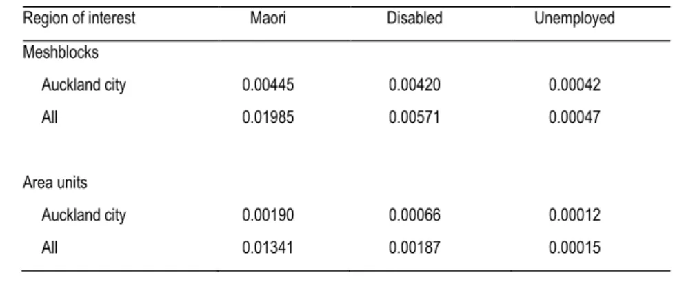
Table 5.2 shows the PWVar for three person-level characteristics. Table 5.2

PWVar for Selected Person Characteristics

A set of simulations were run with just the minimum population threshold (household size) constraint and the homogeneity constraint in place. Using these input parameters, we obtained the results in figures 5.8 and 5.9 for both the dwelling type and the person-characteristic runs, most of the categories exhibit a positive increase in PWVar. AZT was successful in producing a more homogenous set of output zones.

Figure 5.8

PWVar Increase – Dwelling Type

We can also see that the homogeneity results for Auckland city territorial authority are in many cases better than the corresponding results for all of New Zealand. Part of the reason for this may be that Auckland city has many more small meshblocks, and this allows AZTool greater freedom (that is, more possible choices for joining meshblocks together) when it is trying to optimise regions with respect to homogeneity. Ideally, the best set of building blocks for producing output geographies would consist of single-dwelling ‘blocks’ which can be joined together. Another possibility could be that the scale of variation of the homogeneity variables in the city is better captured by the urban meshblocks than it is by their rural counterparts, resulting in better scores.

Figure 5.9

PWVar Increase – Person Characteristics

Other Private Separate House Joined Private Non-permanent Special Dwellings

Relative increase in PWVar over AU geography

P ropor tion i nc reas e -0 .4 -0 .2 0 .0 0 .2 0 .4 0 .6 0 .8 Auckland City All NZ

Maori Disabled Unemployed

Auckland City All NZ

Relative increase in PWVar over AU geography

P ropor tion in cr ea se 0. 0 0. 2 0. 4 0. 6 0. 8

Optimised Geographies for Data Reporting by Martin Ralphs and Lyndon Ang

When additional constraints are included as an AZT run parameter, the resulting output zones are less homogenous. This is to be expected given that the various constraints are competing against each other during the optimisation process (see section 6.1.3 for an example with the population and shape constraints).

When we incorporate all the available constraints (population, shape compactness, and homogeneity) into the AZT optimisation, the PWVar score decreases even further. Again, this is as expected. As table 5.3 shows, AZT with all the constraints enabled produces output zones which are in general less homogenous than the original 2006 Census area units, although these differences are usually quite small.

Table 5.3

Comparing PWVar Values for Area Units and Output Zones

Built With Different Sets of Constraints

Dwelling type Original area units Population and

shape constraints All constraints

Other private 0.00016 0.00014 0.00015

Separate house 0.00417 0.00389 0.00399

Joined private 0.00373 0.00357 0.00375

Non permanent 0.00007 0.00002 0.00002

Special dwelling 0.00002 0.00001 0.00001

The centre column of table 5.3 contains the PWVar values for AZTool runs using only the population and shape constraints. The level of homogeneity for these output geographies is slightly less than those in the right most column when we include the homogeneity constraint. The use of the homogeneity constraint still results in a better level of homogeneity than when we do not use it.

The above results appear to concur with previous work completed in the United

Kingdom, which found that the target population objective function appears to dominate when determining the level of homogeneity possible within the output zones. Larger areas tend to be more homogenous with each other compared to smaller areas. Additionally, for a given target population constraint to be met, AZT will only have a limited number of options to form new output zones such that this constraint is met – this may curtail its ability to also enhance homogeneity. If we have smaller building blocks, we would increase the freedom that AZT has to form output zones, and may be able to increase the level of homogeneity in our output zones.

A final experiment with the homogeneity option involved looking at whether the use of homogeneity variables with a zero or negative correlations between them would have any adverse impact on the results. We calculated correlations between the various homogeneity variables, and chose two pairs to test – one pair having close to a zero correlation, and one with a very weak negative correlation.

The results obtained from AZT contain little evidence to suggest that either a negative or zero correlation between homogeneity variables would perform better than the other.

5.5

Use of the simulated annealing option

It was expected that the use of simulated annealing would improve AZT’s performance. This program option should increase the range of solutions that can be generated, and in consequence improve the quality of the final output. However, in comparing the values of the objective functions with and without Simulated Annealing, we found no gain from using the option.

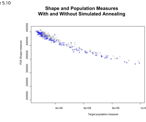
Figure 5.10 plots the shape and population objective function values obtained as AZT progressed. Each point on the graph is an instance where AZT found an improvement in the objective functions, for both the simulated annealing (grey) and non-simulated annealing (blue) runs. Improvements within the first 20 iterations are coded with a circle, while improvements after 20 iterations are coded with a triangle. As the algorithm progresses, the output geographies tend to be more effective in terms of achieving the target population size, but at the cost of less compact shapes. As can be seen, the grey simulated annealing points are consistently above the blue non-simulated annealing points. For a given value of the target population measure, simulated annealing results in less optimal shapes. The simulated annealing option in AZT does not appear to provide a performance gain, at least within 50 iterations.

Figure 5.10

Shape and Population Measures

With and Without Simulated Annealing

Another drawback of using the simulated annealing option is that the minimum population constraint is not met. None of the runs which used the simulated annealing option were able to ensure that all the resulting output zones were above the minimum threshold.

4e+08 6e+08 8e+08 1e+09

200000 250000 300000 350000 400000 450000

Target population measure

P 2A S hape m easu re

Optimised Geographies for Data Reporting by Martin Ralphs and Lyndon Ang

5.6

Optimising all of New Zealand versus a single

region

AZT provides the option to constrain the aggregation of building blocks to fit within pre-defined higher-level geographies. If this option is specified, AZT provides a further option to either perform the aggregation for a single region only, or for all regions

simultaneously within the higher-level geography.

Optimising each region separately may result in more successful local output

geographies. This is because AZT would only need to perform an aggregation for one region at a time, and the resulting local optimisation criteria might potentially provide a better local solution than could be achieved using a New Zealand-wide global score. We wanted to test the validity of this assumption. Some runs were executed to create output zones for the Wellington city territorial authority, in order to test this theory. Fifteen iterations were used for these runs, and the meshblock pattern within Wellington city territorial authority was used as the building block geography.

An AZT run on the single region on our hardware configuration took about five minutes. The length of time increased if multiple runs were being executed at the same time. Given that there are about 73 TAs, and assuming that run times for other regions are also about five minutes, it would take about 6 hours and 5 minutes in total for all the TAs to be processed. In comparison, a 15-iteration AZT run on the whole of New Zealand takes on average about 1 hour and 20 minutes. The reason for this disparity probably lies in the high initial processing overhead of contiguity setup and initial random aggregations that are required on each program restart.

Figure 5.11 shows the empirical distribution of the minimum population size achieved for the Wellington city territorial authority, when AZT aggregates all regions, and also when AZT aggregates just a single region. In terms of the achieved minimum output zone population sizes, AZT successfully meets the minimum population threshold whether it is aggregating a single region or the whole of New Zealand.

Figure 5.11

Distribution of Minimum Population Sizes

Wellington city territorial authority

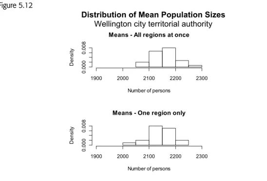
Figure 5.12 shows the distribution of mean population size for both methods. Again, the two distributions are fairly similar in terms of shape and range of values. When

aggregating a single region, AZT appears to be doing slightly better in terms of achieving the target population, as its distribution is located slightly to the left of the distribution achieved when AZT aggregates for the whole of New Zealand. It appears that, at least on average, aggregating a single region at a time produces a slight improvement in terms of achieving the target population.

Figure 5.12

Distribution of Mean Population Sizes

Wellington city territorial authority

Minimums - All regions at once

Number of persons D ens ity 1000 1200 1400 1600 1800 2000 0. 0000 0. 00 15

Minimums - One region only

Number of persons D ens ity 1000 1200 1400 1600 1800 2000 0. 0000 0. 0015

Means - All regions at once

Number of persons De ns ity 1900 2000 2100 2200 2300 0 .00 0 0. 0 08

Means - One region only

Number of persons De ns ity 1900 2000 2100 2200 2300 0 .00 0 0. 0 08

Optimised Geographies for Data Reporting by Martin Ralphs and Lyndon Ang

When AZT aggregates a single region only, the shape compactness of the resulting output zones are similar to the shape compactness of the output zones produced when AZT aggregates the whole of New Zealand. Both of the AZT aggregation methods produce less compact shapes compared to the original area unit distribution.

While it appears that aggregating a single region at a time provides a slight improvement in terms of achieving the target population size, this improvement comes at the expense of a much longer equivalent run time. It would take over four times as long to complete the production of an entire New Zealand output zone geography when we optimise one territorial authority at a time. The lack of a batch mode for AZT (which could be

overcome by further modification of the source code) means that the user would need to manually specify runs for each territorial authority, one at a time.

For the amount of time needed to create a new output geography using one territorial authority at a time, we would be able to create four output geographies by optimising all regions at once. Given the considerable overlap in the output zone distributions in terms of shape and population size, it appears to be more efficient to optimise all regions at once.

One possible option could be to complete a set of AZT runs, where each optimises for the whole of New Zealand. For each territorial authority, we would have a set of output zones from each run. We can compare the objective function values for each set, and select the best set of output zones within each territorial authority. These would then form the final output geography.

As outlined in section 2, the 2006 area unit geography exhibits some problems as the main set of spatial units for disseminating census information. The geography was created over 20 years ago, and no longer reflects real communities or the needs of key users. In addition, the wide range of population sizes and the large number of units with very small populations creates problems of disclosure risk.

Figure 6.1 shows the distribution of 2006 area unit population sizes for New Zealand (excluding meshblocks that are outside the territorial authorities.). The figure highlights some of the problems with the current area unit geography; specifically, that there are a significant number of area units with zero- or very small-sized populations, and the distribution of area unit sizes covers a large range. A small number of area units have very large populations. This poses problems both in terms of data confidentiality as well as data utility.

Figure 6.1

2006 Area Unit Population Distribution

Table 6.1 contains some summary statistics about the 2006 area unit geography. These statistics further highlight the inadequacies of this geography for data output.

Table 6.1

Attributes of 2006 Area Unit (AU) Geography

Attribute Value

Minimum AU size 0

Mean AU size 2,099

Maximum AU size 9,028

Standard Deviation of AU size 1,634

Camden (2008) proposes some guidelines for appropriate population sizes of census output geographies and output classification structures – although they do not consider geographical shape compactness or homogeneity constraints. Meeting the population constraints will require the generation of two new classifications (output area 1 (OA1) and output area 2 (OA2)) to replace the existing meshblock and area unit geographies

Area Unit Population Distribution

Area Unit Size

N um be r of A rea U ni ts 0 2000 4000 6000 8000 10000 0 50 100 20 0

Optimised Geographies for Data Reporting by Martin Ralphs and Lyndon Ang

respectively. He also recommends a set of usually resident person and household sizes for the new geographies. These are given in table 6.2. The proposed size limits are intended to remove problems associated with table sparsity and disclosure risk. Table 6.2

Population and Household Size Targets

Minimum Mean Maximum

‘Meshblocks’ (OA1)

UR Persons 50 100 200

Household 20 40 80

‘Area units’ (OA2)

UR Persons 1,000 2,000 4,000

Household 400 800 1,600

The AZT runs from this project made use of these parameters. In particular, the output geographies we report on in sections 5, 6 and 7 were created using the population minimum and mean values for area units and meshblocks.

The rest of section 6 discusses results obtained from using AZT to create new output zones as an alternative to area units. We refer to these new zones throughout the chapter as OA2 zones. We consider how effective AZT is at creating compact output zones which meet a minimum and target population constraint. We also compare our new OA2 output zones with the original area unit geography. We used the 2006 meshblock pattern as the ‘building block’ geography in generating OA2 zones.

6.1

Simulation results

A number of AZT simulations were performed to test how well the software created new output zones. Over a number of repeated runs, AZT is very consistent in producing output geographies – the final values of the population, shape, and homogeneity constraint after fifteen iterations are very similar across multiple runs. AZT successfully constrains each new OA2 output zone to lie within a single territorial authority.

6.1.1 Ability to meet minimum population size criterion;

using population size as the population constraint

When population size is used as the AZT population constraint, AZT successfully produces OA2 output zones which meet the minimum population threshold of 1000 residents, while also coming close to the target population threshold of 2,000 people. In a set of thirty runs of the program over fifteen iterations per run, with the shape and population constraints in place, all of the runs met the minimum population threshold. Additionally, the mean population size was about 2,200 persons, which was fairly close to the target. In figure 6.2 we show the distribution of the mean and minimum

population size for these runs. The consistency of the outputs in terms of population mean and minimum is apparent.

Figure 6.2

Distribution of Population Size Minimums (left) and Means (right)

For area unit equivalent output zones with a target population size of 2000

Output zones are constructed from meshblocks.

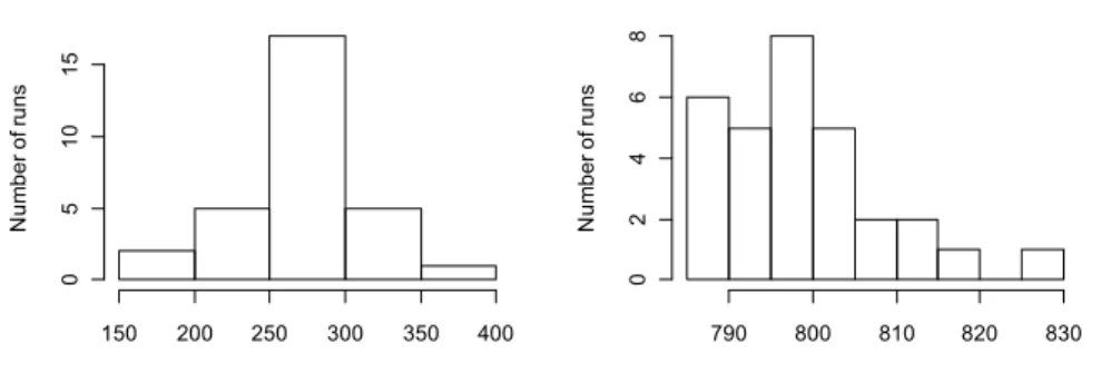
Figure 6.3 shows the distribution of minimum household sizes over the thirty AZT runs. When person size is used as the population constraint, the minimum household size (as specified in table 6.2) will not be able to be satisfied.

Figure 6.3

Distribution of Household Size Minimums (left) and Means (right)

For area unit equivalent output zones with a target household size of 800

Distributions are generated from 30 AZT runs with 15 iterations per run

Output zones are constructed from meshblocks.

6.1.2 Ability to meet minimum population size criterion;

using household size as the population constraint

When we used household size as our population constraint, we found that in addition to meeting the household size criterion, the resulting output geography would usually also meet the minimum resident population size criterion. This is very encouraging, given that we can only apply one minimum population objective function in AZT. We ran six simulations to test this parameter. The minimum household size constraint was met in

Distribution of person size minimums

Number of persons N um ber o f r uns 1000 1050 1100 1150 1200 1250 1300 02 46 8 1 0 1 2

Distribution of person size means

Number of persons N um ber o f r uns 2160 2200 2240 2280 02 46 8 1 0 1 2

Distribution of household size minimums

Number of households N um ber of r un s 150 200 250 300 350 400 0 5 10 15

Distribution of household size means

Number of households N um ber of r un s 790 800 810 820 830 02 4 6 8

Optimised Geographies for Data Reporting by Martin Ralphs and Lyndon Ang

all cases, and only one of them did not also meet the minimum resident population size criterion. Even then, the output tract in question had a population of over 900 persons, which is very close to the minimum size that we are looking for.

The OA2 zones generated by AZT using a minimum household size population constraint usually contain more residents than zones produced with residential population size as the population constraint. For example, in one run using the household size constraint, the minimum output tract size was 1,086 persons, and the mean tract size was 2,476. This mean is about 200 persons higher than typical results obtained using resident population as the population size constraint. For this run, the minimum household size was 430 and the mean household size was 893.

6.1.2.1 Shape compactness of new area units

We assess the shape compactness of OA2 output zones using the P2A measure that was defined in section 5.1. Figure 6.4 contains the shape compactness distribution for a typical AZT OA2 geography generated to replace area units. This geography was

produced using a meshblock contiguity file which excluded single point contiguities. The shape compactness distribution for the official 2006 area unit geography is also

included in light grey for comparison purposes.

AZT output geographies are fairly compact in shape – most output zones have a P2A value that is less than 5. On the other hand, the distribution of P2A values has a long tail. It is evident that the AZT output geography is less compact in shape compared with the original area unit geography. We note that the area unit geography contains areas with P2A values greater than 100, while the maximum P2A value for the AZT geography was about 35.

Figure 6.4

Compactness Distributions – Area Units Versus AZT OA2 Output Zones

Note: Areas with P2A greater than 30 have been excluded from this graph.

Figure 6.5 shows a portion of the OA2 geography from one of our AZT runs, for part of the Wellington city territorial authority. The output zone shapes generated by AZT are in general fairly co