Support Vector Regression Based GARCH Model with Application to Forecasting Volatility of Financial Returns

SFB 649 Discussion Paper 2008-014

Support Vector Regression

Based GARCH Model with

Application to Forecasting

Volatility of Financial

Returns

Shiyi Chen*

Kiho Jeong**

Wolfgang Härdle***

*Fudan University Shanghai, China ** Kyungpook National University Daegu, Korea

*** Humboldt-Universität zu Berlin, Germany

This research was supported by the Deutsche

Forschungsgemeinschaft through the SFB 649 "Economic Risk". http://sfb649.wiwi.hu-berlin.de

ISSN 1860-5664

SFB 649, Humboldt-Universität zu Berlin Spandauer Straße 1, D-10178 Berlin

S

FB

6

4

9

E

C

O

N

O

M

I

C

R

I

S

K

B

E

R

L

I

N

Support Vector Regression Based GARCH Model with

Application to Forecasting Volatility of Financial Returns

#

Shiyi Chen

*

，

Kiho Jeong

**

and Wolfgang Härdle

***

January, 2008

ABSTRACT

In recent years, support vector regression (SVR), a novel neural network (NN) technique, has been successfully used for financial forecasting. This paper deals with the application of SVR in volatility forecasting. Based on a recurrent SVR, a GARCH method is proposed and is compared with a moving average (MA), a recurrent NN and a parametric GACH in terms of their ability to forecast financial markets volatility. The real data in this study uses British Pound-US Dollar (GBP) daily exchange rates from July 2, 2003 to June 30, 2005 and New York Stock Exchange (NYSE) daily composite index from July 3, 2003 to June 30, 2005. The experiment shows that, under both varying and fixed forecasting schemes, the SVR-based GARCH outperforms the MA, the recurrent NN and the parametric GARCH based on the criteria of mean absolute error (MAE) and directional accuracy (DA). No structured way being available to choose the free parameters of SVR, the sensitivity of performance is also examined to the free parameters.

Keywords: recurrent support vector regression; GARCH model; volatility forecasting

JEL classification: C45, C53, G32

#

This work was supported by Deutsche Forschungsgemeinschaft through the SFB 649 "Economic Risk". Shiyi Chen was also sponsored by Kyungpook National University Graduate Scholarship for Excellent International Students and Shanghai Pujiang Program. * (Corresponding author) China Center for Economic Studies (CCES), Fudan University, Shanghai 200433, China; Email: [email protected]; TEL: +86 21-6564-2050

** School of Economics and Trade, Kyungpook National University, Daegu 702-701, Korea Email: [email protected]; TEL: +82 53-950-5416

*** Center for Applied Statistics and Economics (CASE), Department of Economics, Humboldt-Universität zu, D-10178, Berlin, Germany; Email: [email protected]; TEL: +49 30 20 93 56 31

I. INTRODUCTION

Volatility is important in financial markets since it is a key variable in portfolio optimization, securities valuation, and risk management. Much attention of academics and practitioners has been focused on modeling and forecasting volatility in the last few decades. So far in the literature, the predominant model of the past was GARCH model by Bollerslev (1986), who generalizes the seminal idea on ARCH by Engle (1982), and its various parametric extensions. The popularity of GARCH model is due to its ability to capture many of the empirically stylized facts of financial time series, such as time-varying volatility, persistence and volatility clustering (Marcucci, 2005); see Bollerslev, Chou and Kroner (1992) for literature surveys.

Evidence on the forecasting ability of GARCH model is somewhat mixed. Anderson and Bollerslev (1998) show that GARCH model provides good volatility forecast. Conversely, some empirical studies show that GARCH model tends to give poor forecasting performances; for example, Figlewski (1997), Cumby et al. (1993), Jorion (1995, 1996), Brailsford and Faff (1996), and McMillan et al. (2000).

To improve the forecasting ability of GARCH model, some alternative approaches have been advocated from the perspective of estimation and forecasting. Neural network (NN) is one such method. In recent years, NNs have been successfully used for forecasting financial time series; for recent work, see Fernandez-Rodriguez et al. (2000) and Refenes and White (1998). The main appeal of NNs is their flexibility in approximating any non-linear function arbitrarily well without a priori assumptions about the properties of the data; see Hornik et al. (1989) for a discussion of the NN universal approximation property. Motivated by their good property and promising results in a broad range of financial applications, various NN-based GARCH models have been suggested and applied to forecasting volatility. The basic finding supports that NN-based GARCH outperforms traditional GARCH models in forecasting conditional volatility; see Donaldson and Kamstra (1997), Schittenkopf et al. (2000), Taylor (2000), Dunis and Huang (2002). However, NN suffers from a number of weaknesses including the need for a large number of controlling parameters, difficulty in obtaining a global solution and the danger of over-fitting (Tay and Cao, 2001). The over-fitting problem is a consequence of the optimization algorithms used for parameter selection and the statistical measures used to select the best model.

Recently, a novel NN algorithm, called support vector machine (SVM), was developed by Vapnik and his co-workers (1995, 1997) and is gaining popularity due to many attractive features. While the traditional NN implements the empirical risk minimization (ERM) principle, SVM implements the structural risk minimization (SRM) principle which seeks to minimize an upper bound on the Vapnik-Chervonenkis (VC) dimension (generalization error), as opposed to ERM that minimizes the error on the in-sample estimating data;, refer to Gunn (1998) for a good introduction to SVM and related concepts. Based on SRM principle, SVM achieves a balance between the training error and generalization error, leading to better forecasting performance than traditional NN. Selecting the best model in SVM is equivalent to solving a quadratic programming, which gives SVM another merit of a unique global solution. SVM was originally developed for classification problems (SVC)

and then extended to regression problems (SVR).

The main purpose of this paper is to formulate some types of SVR-based GARCH models and to compare the forecasting performance to the results obtained from a moving average (MA), a recurrent NN and a parametric GACH (MLE). Recently, Pérez-Cruz et al. (2003) also proposed a SVR-based GARCH(1,1) model and showed that the proposed method provided better volatility forecasts than parametric GARCH model. However, they used feedforward SVR procedure which has the same structure as autoressive (AR) process and has poor ability to model the long-time memory (Haykin, 1999). In this paper, we apply the recurrent SVR procedure, firstly proposed by Chen and Jeong (2005), which can introduce ARMA structure into either mean function or conditional variance. The criteria of mean absolute error (MAE) and directional accuracy (DA) reveal that recurrent SVR-based GARCH model outperforms MA, MLE and NN-based GARCH model in the one- and multi-period-ahead forecasts of volatility. This paper is organized as follows. Section 2 introduces the theory of SVR. Section 3 specifies the empirical model and forecasting scheme. Section 4 uses the Monte Carlo Simulation to evaluate how the models perform under controlled conditions. Section 5 describes the GBP exchange rates and NYSE composite index data and discusses the volatility forecasting performance of all models for real data. This paper concludes in section 6.

II. SUPPORT VECTOR REGRESSION

SVR performs by nonlinearly mapping the input space into a high dimensional feature space and then runs the linear regression in the output space. Thus, linear regression in the output space corresponds to nonlinear regression in the low dimensional input space. As the name implies, the design of the SVR hinges on the extraction of a subset of the training data that serves as support vectors and that therefore represents a stable characteristic of the data. Given a training data set

{

(

)

}

1

,

N

t t _t

x y

₌ , with vector inputs , scalar outputs , and unknown function , we need to estimate a decision function

0 m t x ∈\

y

t

∈

\

( )

g x

f x

( )

that approximates

g x

( )

as below.

( )

1

( )

( )

1 m T j j j

f x

w

ϕ

x

b

w

ϕ

x

=

=

∑

+ =

+

b

1 1 T m ⎤⎦ " (1)

where

( )

( )

( )

. The nonlinear function

1 1 , , , , , T m x x x w w w

ϕ

=⎡_⎣

ϕ

"

ϕ

⎤_⎦ =⎡_⎣

ϕ

j

( )

x

is the features of the input space, in SVR jargon. The dimension of the feature space is which is directly related to the capacity of the SVR to approximate a smooth input-output mapping; the higher the dimension of the feature space, the more accurate the approximation will be. Parameter denotes a set of linear weights connecting the feature space to the

1

m

i

output space, and b is the bias. Using the decision function

f x

( )

, we can achieve the best generalization capability in forecasting y on new inputs.

In order to derive the decision function, coefficients and b have to be estimated from the data. First, we define a linear

i

w

ε

-insensitive loss function,

L

_ε

(

x y f x

, ,

( )

)

, originally proposed by Vapnik (1995),

( )

(

, ,

)

( )

( )

0 y f x for y f x L x y f x otherwise ε

ε

ε

⎧ − − − ≥ ⎪ = ⎨ ⎪⎩ (2)

Under this loss function, errors below

ε

are not penalized; we can ignore the error and say the predicted

f x

( )

has no loss.

The derivation of SVR follows the principle of structural risk minimization that is rooted in VC dimension theory. The primal constrained optimization problem of

ε

-SVR is obtained as below. ( )' 2

(

)

(

2 ' ' , , ₁

1

1

min

, , ,

2

N N N t t t t w b _t

w b

w

C

N

ξ

ξ ξ

)

∈ ∈ ∈ ₌

⎛

⎞

Φ

=

+

⎜

+

⎝

∑

⎠

\ \ \

ξ ξ

⎟

N (3)

( )

. .

T _{t t}

1, 2,

,

s t

w

ϕ

x

+ − ≤ +

b

y

ε ξ

t

=

"

N

(4)

( )

'

1, 2,

,

T t t

y

−

w

ϕ

x

− ≤ +

b

ε ξ

t

=

"

N

(5) ' 0, 0 1, 2, , t t t

ξ

≥

ξ

≥ = " (6)

The formulation of the cost function Φ

(

w b, , ,

ξ ξ

t t'

)

in equation (3) is in perfect accord

with the principle of structural risk minimization; see Figure 1 (in which the dark circles are data points extracted as support vectors). In equation (3), the first term, 1 2

2 w , is a measure

of the function flatness, minimizing what is related to maximizing the margin of separation

2 /

w

, i.e., indicates maximizing the generalization ability. The second term describes the

ε

-insensitive loss function (denoted by the nonnegative slack variables

ξ

_i' and

ξ

_i) and is similar to, although not identical with, the empirical risk employed in NN

The corresponding dual problem of nonlinear SVR can be derived using the Karush-Kuhn-Tucker conditions as follows:

( )' 2

(

)(

)

(

)

(

)

(

' ' ' ' 1 1 1 1 1 min 2 N N N N N

)

s s t t s t t t t t t s t t t K x x y α ∈\

∑∑

_{= =}

α α α α

− − ⋅ +

ε

∑

₌

α α

+ −

∑

₌

α α

− (7)

(

'

)

1 . . 0 N t t t s t

α α

= − =

∑

(8) ' 0 _t, _t C s t, 1, 2, ,N N

α α

≤ ≤ = " (9)

where,

α

_t' and

α

_t are the Lagrange multipliers. The dual problem is easier to solve than the primal problem by relying on a quadratic programming (QP) scheme (Scholkopf and Smola, 2001; Deng et. al., 2004). We can then use them to obtain the solution of the primal problem:

(

'

)

( )

1 N t t _t t w

α α ϕ

= =

∑

− x (10)

(

'

)

(

)

(

'

)

(

)

1 1

1

x x

x x

2

N N t t t t j k t j t k t t

b

y

y

α α

K

α α

K

= =

⎡

⎛

⎞

⎤

=

⎢

+

−

⎜

−

⋅

+

−

⋅

⎟

⎥

⎝

⎠

⎣

∑

∑

⎦

(11) , for j, 'k 0, C N

α α

_∈⎜⎛ ⎞_⎟ ⎝ ⎠

Substituting equation (10) and equation (11) into equation (1), the decision function can be obtained:

( )

(

'

)

( ) ( )

(

'

)

(

)

1 1 , N N T t t _t t t _t t t f x

α α ϕ

x

ϕ

x b

α α

K x x b = = =

∑

− + =

∑

− +

)

)

, (12)

where is the kernel function. The SVR theory considers the form of in the feature space without specifying

(

t

,

)

T

( ) (

t

K x x

=

ϕ

x

ϕ

x

(

_t

,

K x x

ϕ

( )

x

explicitly and without computing all the corresponding inner products. Therefore, kernels provide the flexibility of the high dimensional feature space for low computational costs and are a crucial part of SVR. No analytical method is currently available to determine the most suitable kernel for a particular data set. This paper experiments with three different kernels to investigate the effect of a kernel type.

Linear:

K x x

(

_t

,

)

=

x x

_tT (13) Polynomial:

K x x

(

_t

,

)

=

(

x x

_tT

+

1

)

d (14) Gaussian:

(

)

2 2

,

exp

2

t t

x

x

K x x

σ

⎛

− −

⎞

=

⎜

⎜

⎝

⎠

⎟

⎟

(15)

III. EMPIRICAL MODELING AND FORECASTING SCHEME

In this paper, the data we analyze is just the daily financial returns,

y

_t, converted from the corresponding price or index,

I

_t, using continuous compounding transformation as

(16)

(

1

100

log

log

t t

y

=

×

I

₊

−

I

_t

)

t

A GARCH (1, 1) specification is the most popular form of conditional volatility. As such, throughout the paper the analysis is restricted to the case of GARCH (1,1) process.

The Linear and Nonlinear GARCH (1, 1) Models

For the parametric GARCH model, GARCH (1,1) model is usually specified as follows: 1 1 t t

y

= +

c

φ

y

₋

+

u

(17-1) (17-2) 2 1 1 1 1 t t h = +

κ δ

h₋ +

α

u_t−

The important point is that the conditional variance of

u

_t is given by

h

_t

=

E u

_{t−1 t}2

=

u

t t2| 1− .

Thus, the conditional variance of is the ARMA process given by the expression in equation (17-2) (Bollerslev, 1986; Hamilton, 1997; Enders, 2004).

t

u

h

t (18)

(

)

2 2 1 1 1 1 t t t

u

= +

κ

δ α

+

u

₋

+

w

−

δ

w

_t−1

2 2 2 | 1 t t t t t

w

≡

u

−

u

−

=

u

−

h

_t

where

w

t is white noisy errors. The parameters

κ δ

,

1and

α

1 must satisfy

κ

>

0

, 1

0

δ

≥

, and

α

₁

≥

0

to ensure that the conditional variance is positive. Together with the nonnegative assumption, if

δ α

₁

+

₁

<

1

, then u_t2 is covariance stationary.

For recurrent SVR and NN methods, the nonlinear AR(1)–GARCH(1,1) model has the following form: (19-1)

( )

1 t t

y

=

f y

₋

+

u

_t t + (19-2)

(

)

2 2 1, 1 t t t u =g u₋ w₋ w

Recurrent SVR-based GARCH Modeling and Forecasting Scheme

The algorithm of the recurrent SVR-based GARCH model is described as follows:

STEP 1: run the SVR-based AR(1) model for returns

y

_t in the full sample period T,

( )

1

(

1, 2,

,

t t t

y

=

f y

₋

+

u

t

=

"

T

)

)

t , to obtain residuals,

u u

₁

,

₂

,

"

,

u

_T.

STEP 2: recursively run the recurrent SVR for squared residuals, with updating,

(

1 2 2 2 1

,

2

,

,

T 1

u u

"

u

T

<

T

(

)

2 2 1, 1 t t t u =g u₋ w₋ +w

to obtain 60 one-period-ahead forecasted volatilities. 1 1 1 2 1 1 2 1 1 1 2 59 1 1 1 : 1, 2, , 2 : 1, 2, , 1 60 : 1, 2, , 59 T T T st sample t T u nd sample t T u th sample t T u + + + + + = → = + → = + → " " "" "

STEP 3: run the recurrent SVR for squared residuals,

(

)

2

2 2 2

1

,

2

,

,

T 2

20

u u

"

u

T

= −

T

, without

updating to obtain 20 multi-period-ahead forecasted volatilities.

2 2 2 2 2 2 1 2 2

:

1, 2,

,

T

,

T

,

,

T

estimating sample t

=

"

T

→

u

+

u

+

"

u

+20

For each of 60 estimations, the recurrent SVR procedure proposed by Chen and Jeong (2005) is run as follows; the residuals of

w

_t−1 in equation 19-2 are first set to be zero series; then

run the feedforward SVR to obtain estimated residuals; using the estimated residuals as new inputs we can carry out this process repeatedly until the stopping criterion is satisfied.

1 t

w

₋

The appropriate parameter

ε

dramatically depends on the given data but is not very sensitive to the same data; after investigation, we choose

ε

=

0.0001

for simulation data and

ε

=

0.05

for real data. The value of C has been set to 0.1 for both data because investigation reveals that the solution is not very sensitive to C for a wide range. In addition, the fixed width value of 0.2 for Gaussian kernels and d=2 for polynomial kernels, are also set for the convenience of comparison.

Evaluation Measures and Proxy of Actual Volatility

We evaluate the forecasting performance using two standard statistical criteria: mean absolute forecast error (MAE) and directional accuracy (DA), expressed as follows (Brooks, 1998; Moosa, 2000):

2 2 1

1

n i i i

MAE

u

u

n

=

=

∑

−

(20)

( )

1 100 % n i i DA a n = =

∑

(21) where

(

)

(

2 2

)

2 2 1 1

1

0

0

i i i i i

u

u

u

u

a

otherwise

+ +

⎧

−

−

⎪

= ⎨

⎪⎩

≥

MAE measures the average magnitude of forecasting error which disproportionately weights large forecast errors more gently relative to MSE; and DA measures the correctness of the turning points forecasts, which gives a rough indication of the average direction of the forecasted volatility.

The fundamental problem with the evaluation of volatility forecasts of real data is that volatility is unobservable and so actual values, with which to compare the forecasts, do not exist. Therefore, researchers are necessarily required to make an auxiliary assumption about how the actual ex post volatility is calculated. In this paper, we use square of the return minus its mean value as the proxy of actual volatility against which MAE and DA can be calculated. This approach is similar to the standard one, squared returns, because the mean of returns is usually close to zero. The proxy of actual volatility in real data is expressed as

(

2

2

t t

u

=

y

−

y

)

(22)

This proxy has been used in many recent papers such as Pagan and Schwert (1990), Day and Lewis (1992), Chan et al. (1995), West and Cho (1995), Chong et al. (1999), Brooks (2001), and Brooks and Persand (2003).

Specification of other Methods

The MA method uses weighted moving averages of past squared innovations to forecast volatility (Niemira and Klein, 1994). For simulated data, the MA forecast for the next-day volatility, using the 5 most recent observations, is expressed as

2 2 5, 1 4

1

5

t t _j j t

u

+ = −

=

∑

u

(23)

For real data, the MA forecast for the next-day volatility is expressed as (Engle et al., 1993)

2

(

2 5, 1 _5, 4

1

5

t t _{j t} j t

u

+

y

= −

=

∑

−

y

)

(24) where _5, 4

1

5

t j t j t

y

y

= −

=

∑

.

The recurrent networks experimented in this study are multilayer perceptrons (MLP) and a radial-basis function (RBF) network with the addition of a global feedback connection from the output layer to its input space. We specify a MLP network with the following architectures: one nonlinear hidden layer with 4 neurons using a tan-sigmoid differentiable transfer function, and one linear output layer with 1 neuron. The fast training Levenberg-Marquardt algorithm is chosen and designed into a training function. The value of the learning rate parameter is 0.05. The RBF network used in this study is a generalized regression neural network (GRNN) which also has two layers: the first layer is a radial basis layer whose weights are set to transposed inputs, and the output layer is a special linear layer whose weights are set to target vectors. The spread of the radial basis function is 1.0. These specifications and choices are quite standard in the literature of neural networks.

Empirical Framework

In this study the forecasts are obtained by applying the Monte Carlo method1, following the suggestions in Andersen and Bollerslev (1998), and Clements and Smith (1999, 2001). The main motivation for conducting a simulation experiment is that, since the true volatility is known, the candidate volatility measures can be compared with certainty. We also fit each of

1

the models to the daily returns on the GBP exchange rate and NYSE stock indexes and forecast their respective volatility. The empirical modeling and forecasting scheme described above are employed for both simulation and real data. The results in this paper are calculated via MATLAB 7.0 software.

IV. MONTE CARLO SIMULATION

In this section we investigate the forecasting performance of all candidates using artificial simulated data under controlled conditions. To generate the data, we first need to parameterize the GARCH (1,1) model in equations (17) with the following settings

for medium persistence and a disturbance term distributed first as Gaussian and then as a Student's t with five degrees of freedom (kurtosis = 5). The second distribution tries to model the excess of kurtosis that usually appears in real financial series. Using the same specified models, two artificial samples with sizes, 500 and 1000, are created under two distributions assumption, giving a total of four situations. To limit the computational burden, each situation is replicated only 50 times. Then the multiple simulated

(

c

, , , ,

φ κ δ α

1 1 1

) (

=

0, 0.5, 0.0005, 0.8, 0.1

)

t

u

t

y

and are 500-by-50 and 1000-by-50 element matrices for different distribution.

t

h

For each replication, the recurrent SVR-based GARCH(1,1) model and others are estimated and forecast errors are calculated using the forecasting schemes described in Section 3. We have reported the results of one-period-ahead forecasting measures for four situations, respectively, in Tables I (a) and (b) and 20-period-ahead forecasting results in tables II (a) and (b). The reported results are the mean values of 50 independent replications.

[Tables I (a) and (b)]

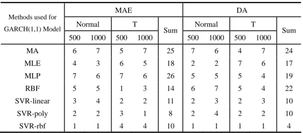
Let us first evaluate the one-period-ahead forecasts using the updating forecasting scheme described in Table I. In terms of the sum rankings of MAE measures, the order of the forecasting ability of the different methods from the highest to lowest is displayed in turn as follows: poly-SVR, rbf-SVR, linear-SVR2, RBF, MLE, MA and MLP. Concretely, in the situation of normal distribution, MLE which is ranked fourth behaves not bad and is only inferior to the three kinds of SVR methods in the 500 sizes, and even ranked third, is only defeated by poly- and rbf-SVR in the 1000 sizes. As well, the MAE values of rbf-, poly-, and linear-SVR and MLE are also close, for example, 0.0000796, 0.0000924, 0.0000960 and 0.0000972, respectively, for the 500 sizes, and 0.0000456, 0.0000479, 0.0000501 and 0.0000488 for the 1000 sizes; the latter of which becomes smaller for all methods when the sizes of the sample increase. However, one thing noteworthy here is that even though the data satisfy the Gaussian assumption, the SVR methods still outperform MLE in forecasting volatility error magnitude. In the situation of t distribution, the forecasting performance of MLE grows

2

poorer, only ranked second last for the 500 sizes and third last for the 1000 sizes, and the difference of MAE values between SVR and MLE becomes larger. For instance, the values of three kinds of SVR are all below 0.00014 for the 500 sizes and below 0.000077 for the 1000 sizes, while those of MLE are 0.0001765 and 0.0001083, respectively. The performance of NN is confusing: MLE is better than MLP but worse than RBF.

According to the sum rankings of the DA measures, rbf-SVR ranks highest for all four situations; linear- and poly-SVR are ranked second side by side; now, MLE is ranked fourth and MA last among all candidates. In the situation of normal distribution, MLE behaves better than in forecasting error magnitude, and is ranked second for the 500 sizes (76.27%) only inferior to rbf-SVR (86.44%) but equal to linear- and poly-SVR (76.27%), and also ranked second for the 1000 sizes (79.83%) only inferior to rbf-SVR (83.05%) but better than linear- and poly-SVR (74.58% and 71.19%). These values of SVR and MLE are close and, particularly higher than the NN and MA methods. Although good, MLE cannot defeat rbf-SVR even in the case of normal distribution and large sample sizes. As for the situation of t distribution, the parametric GARCH is ranked last for the 500 sizes (55.9%) and second last for the 1000 sizes (59.3%); while for any of the sizes, the three kinds of SVR are always the top three methods in forecasting the volatility direction, all higher than 70% which none of the other methods can reach. This time the NN defeats MLE. As for MLE and MA, in the situation of the 500 sizes and t distribution MLE performs worse than MA in terms of both MAE and DA measures.

[Tables II (a) and (b)]

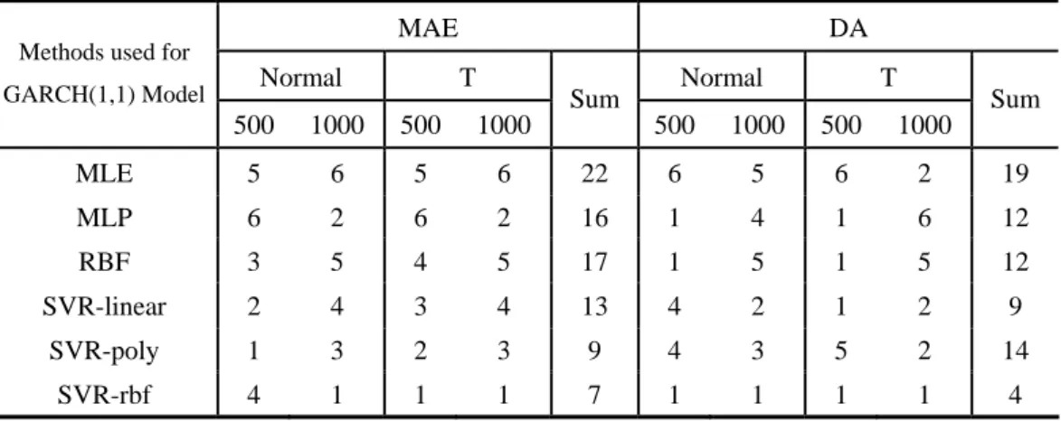
We now assess the performance of the fixed forecasting rule shown in Table II. Based on the sum rankings of the MAE measures, the order of forecasting ability of the different methods from the highest to lowest is displayed in turn as follows: rbf-SVR, poly-SVR, linear-SVR, MLP, RBF and MLE. The special thing impressing us is that the MLE has almost the worst forecasting performance. In the situation of Gaussian distribution, for the 500 sizes, the MAE value of MLE is 0.0014271 and that of rbf-SVR, worst among the three kinds of SVR, is 0.0009955, the difference between them is 0.0004316. For the 1000 sizes, the MAE value of MLE decreases to 0.0004216 and that of linear-SVR, the worst among the three SVR, also decreases to 0.0002006, the difference reduces to 0.000224. Obviously, even if in the case of normal distribution and large sample sizes, SVR still outranks MLE in forecasting volatility error magnitude. In the situation of t distribution, for the 500 sizes, the MAE value of MLE increases to 0.0019922 but that of linear-SVR, the worst among the three kinds of SVR, decreases to 0.0005832, the difference is 0.001409 much larger than that in normal distribution. For the 1000 sizes, the MAE value of MLE is 0.0008628 and that of linear-SVR, the worst among the three kinds of SVR, is 0.0006124, the difference reduces to 0.0002504 which is smaller than the previous one in the 500 sizes but larger than the corresponding one in normal distribution. In a word, in the case of t distribution, the three SVR are greatly superior to MLE, the latter of which grows poorer as it always does. As for NN, SVR also outperforms them for all four situations with just a few exceptions (normal distribution and the 500 sizes for RBF, the 1000 sizes and both distributions for MLP).

According to the sum rankings of the DA measures, rbf-SVR also ranks highest for all four situations, the same as with the updating forecasting scheme; linear-SVR is ranked second; but

poly-SVR is inferior to MLP and RBF; again, MLE is the worst one, the same as that in terms of the MAE criteria. The DA value of MLE in the situation of the 500 sizes and t distribution is only 26.316%, the lowest among all the values; although in the situation of the 1000 sizes and t distribution is 68.421% equal to the linear- and poly-SVR. The worst performance of MLE in the case of both measures denotes that MLE is not suitable for long-run ex ante forecasts. Two NNs hold the same highest position as rbf-SVR in the situation of the 500 sizes and both distribution and as linear-SVR in the 500 sizes and t distribution. But, according to the sum rankings of both MAE and DA measures, three kinds of SVR still outperform two NNs under the fixed forecasting scheme. Taken together, if you want to forecast long-run volatility using a fixed forecasting rule, the recurrent SVR is the first choice, followed by NN, and MLE is the final one.

V. REAL DATA ANALYSIS

The aim of this section is to compare the volatility forecasting performance of different methods for two kinds of financial returns: GBP/USD exchange rates and the NYSE stock index.

Data description

The first data set consists of the daily nominal bilateral exchange rates of British Pounds (GBP) against the U.S. dollar for the period of July 2, 2003 to June 30, 2005. The data are obtained from a database provided by Policy Analysis Computing and Information Facility in Commerce (PACIFIC) at the University of British Columbia, which contains the closing rates for a total of 81 currencies and commodities. The second data set consists of the daily closing price of the New York Stock Exchange TM (NYSE) composite stock index for the period of July 3, 2003 to June 30, 2005. The data are downloaded directly from the Market Information section of the NYSE TM web page.

Both sets of raw real data are transformed into daily returns via equation 16, giving a returns series of 503 observations and then a residual series of the same size is obtained from a fitted conditional mean equation of the GARCH model. For the squared residuals of the 503 observations, the recursive estimating samples for the conditional volatility function are updated from the former 424 observations through the former 483 and then 60 numbers of one-period-ahead forecasts are obtained which correspond to an out-of-sample evaluation sample spanned from the 425th through the 484th data points. The multi-period-ahead evaluation sample is the last 20 observations which span from the 484th data point to the end.

[Figure 2] [Figure 3]

The daily series for the log-levels and the returns of the GBP and NYSE (503 observations) are depicted in Figure 2 and 3, respectively. Both figures show that the returns series are mean-stationary, and exhibit the typical volatility clustering phenomenon with periods of unusually large volatility followed by periods of relative tranquility. Table III reports the summary

of the descriptive statistics for the GBP and NYSE returns. The GBP series are typically characterized by excessive kurtosis and asymmetry. The Bera-Jarque (1981) test strongly rejects the normality hypothesis for GBP. But the NYSE series cannot reject the normality hypothesis. For both series, the Ljung-Box Q(6) statistics of raw returns indicate no significant correlation; but the Q(6) values of the squared returns reveal that there is significant serial correlation in the squared returns. Engle’s (Engle, 1982) ARCH tests show significant evidence in support of GARCH effects (i.e., heteroscedasticity) for both series. This examination of daily returns on the GBP and NYSE data reveals that returns can be characterised by heteroscedasticity and time-varying autocorrelation, therefore, we expect the GARCH models to capture it adequately.

[Table III]

Evaluating the forecasting performance of each method

The results of forecasting accuracy for each model using real data are shown in Table IV for both one- and multi-period-ahead forecasts; where, (a) reports the values of the evaluation measures and (b) is the ranking of all the models.

[Table IV (a) and (b)]

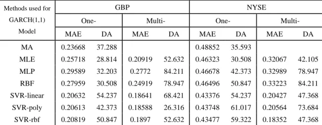
We first evaluate one-period-ahead forecasts of volatility, as described in Table IV. According to the sum rankings of the MAE of two returns, three kinds of SVR are the top three methods, followed by the MLE method which is ranked fourth for the NYSE, characterized by Gaussian distribution, but fifth for GBP returns which show a high excess kurtosis. Obviously, the values of MAE of the three kinds of SVR are below 0.21 and 0.44, respectively, for the GBP and NYSE returns, while those of MLE are 0.25718 and 0.46323. RBF and MA method which are ranked fifth perform equally well while the MLE method is ranked last. Therefore, the values of MAE indicate the smallest deviation between the actual and forecasted volatility for the recurrent SVR method as opposed to the competing methods. In terms of the sum rankings of the DA criteria, the three kinds of SVR also rank the highest among all the methods and perform equally well, followed by MLP, RBF and MA method which are equally ranked fourth side by side. For example, the DA values of the three SVR for both returns all exceed 50%; among the other values, only that of the RBF for the NYSE data is a little more than 50%. MLE method performs worst for both GBP and NYSE returns, the DA values of which are only 28.8% and 30.5%, respectively. Here, MA almost outranks MLE based on two measures only except for the MAE value in the NYSE.

Next, we consider the situation of multi-period-ahead forecasts of volatility. Based on the sum rankings of MAE for the two returns, the three kinds of SVR are also the best methods (the MAE values of which are below 0.19 and 0.21 for GBP and NYSE), followed by MLE (0.20919 and 0.32067 for both data), NN is the worst one (more than 0.24 and 0.329 for the two returns). There is a change in terms of the DA measure. Two kinds of NN rank in the first class, the correctness ratio of which is higher than 78%. Now, the three kinds of SVR rank in the second class in the sum rankings of the two returns. Also, MLE ranks the lowest as it does

in one-period-ahead forecasting. However, in terms of the sum rankings of the MAE and DA measures, the recurrent SVR is still better than the other methods while NN beats back MLE. Taken together, the recurrent SVR consistently being the best in error magnitude and direction forecasts while MLE is always the worst in forecasting the turning points of volatility3 and is only inferior to SVR in forecasting error size. We cannot conclude that NN outperforms MLE overall as argued in other studies.

[Figure 4 (a) and (b)]

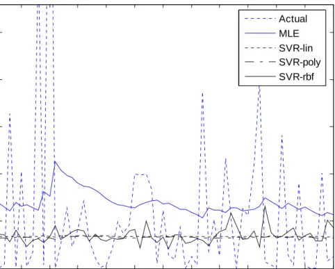
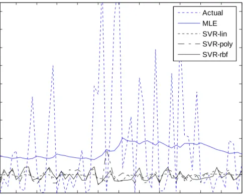
We have plotted the forecasted volatility from three recurrent SVR- and MLE–based GARCH (1,1) models, along with the actual ex-post volatility measures based on the squares of returns minus their means4, for GBP exchange rates and the NYSE stock index in Figures 4 and 5, respectively; in which (a) graphs 60 one-period-ahead forecasts for the out-of-sample period of March 10, 2005 to June 3, 2005 resulting from the updating forecasting scheme, and (b) displays 20 multi-period-ahead forecasts for the out-of-sample period of June 3, 2005 to June 30, 2005 from the fixed rule.

[Figure 5 (a) and (b)]

Seen from (a) and (b) in the two Figures, it is clear that the updating forecasting scheme tracks the ex-post actual volatility better than the fixed one for all the models. For both forecasting schemes, overall, the three kinds of recurrent SVR-based GARCH (1,1) models seem to do a remarkable job of capturing the future volatility clustering effect in two returns in the out-of-sample.

CONCLUSIONS

In many applications, SVR has shown excellent forecasting performance due to its particular design of minimizing structural risk rather than empirical risk employed by neural networks and traditional methods (Vapnik, 1995, 1997). This inspires us to use it to improve the forecasting ability of the traditional GARCH models. In terms of the MAE and DA measures, in this study, we investigate the forecasting ability of the recurrent SVR-based GARCH (1,1) models as compared with MA, recurrent NN and MLE methods by using a Monte Carlo simulation and real data of the British Pound-US Dollar (GBP) daily exchange rates.

The real data results, together with the simulation evidence, consistently support the use of the three recurrent SVR-based GARCH models in forecasting one- and multi-period-ahead volatility error magnitude and direction; although, in the case of forecasting long-term volatility direction, neural networks also perform equally well. As for the performance of the different kinds of SVR, simulation supports poly-SVR but real data analysis favors linear-SVR in one-period-ahead error

3

It is noteworthy that, DA provides a measure of the consistency in the prediction of the volatility direction which may yield important information for financial decisions in risk management field. Therefore, the problem should be considered seriously when using the MLE method.

4

The forecasted volatility from MLP, RBF and MA methods are not plotted just to not make the figure complicated.

size forecasts. Simulation also favors rbf-SVR in short-term volatility direction forecasts and in long-term error size and direction forecasts, the conclusions of which are confirmed by the real data only with the one exception of long-term direction forecasts. Since no single kernel function dominates all predictions, practitioners should try more than one kernel function.

MLE cannot always perform better than SVR even with the required assumptions of Gaussian distribution and large sample sizes being satisfied for data. NN is also inferior to SVR in volatility forecasts. Therefore, it is concluded that the problem of good estimation and poor forecasts can be resolved using our recurrent SVR method. In multi-period-ahead volatility forecasts, particularly noteworthy, MLE almost ranks the lowest among all methods, which indicates that MLE is not suitable for long-run volatility forecasting. Due to the introduction of global feedback loops and the corresponding richer dynamic structures, SVR looks more promising in doing so.

Using the squares of the returns as the proxy of actual data would greatly influence the forecasting evaluation results; therefore, we have left for future work the investigation of an alternative use of cumulative squared returns from high frequency intraday data as the proxy of ex post volatility, following Anderson and Bollerslev (1998). The relative accuracies of the various methods are also highly sensitive to the statistic measures used to evaluate them; therefore, it is generally impossible to specify a forecast evaluation criterion that is universally acceptable. This problem is especially acute in the context of nonlinear volatility forecasting (Engle et al. 1993; Diebold and Mariano 1995; West 1996; Andersen et al. 1999; Dacco and Satchell 1999; and Clements and Smith 2001), which should prompt us to consider more appropriate evaluation criteria that are linked directly to our future applications.

REFERENCES

Database of Exchange Rates: http://pacific.commerce.ubc.ca/xr, Policy Analysis Computing and Information Facility In Commerce (PACIFIC) at University of British Columbia. Database of NYSE stock index: http://www.nyse.com/marketinfo/datalib/, the Market

Information section of the NYSE TM web page.

Andersen TG, Bollerslev T, 1998, Answering the Skeptics: Yes, Standard Volatility Models do Provide Accurate Forecasts, International Economic Review, 39, 885-905

Andersen TG, Bollerslev T, Lange S, 1999, Forecasting financial market volatility: Sample frequency vis-a-vis forecast horizon, Journal of Empirical Finance, 457-477

Bera, A.K. and C.M. Jarque, 1981, An efficient large-sample test for normality of observations and regression residuals, Australian National University Working Papers in Econometrics, 40, Canberra.

Bollerslev, T., 1986, Generalized autoregressive conditional heteroskedasticity, Journal of Econometrics 31, 307-327.

Bollerslev, T., Chou R.Y., and Kroner K.F., 1992, ARCH modeling in finance: A review of the theory and empirical evidence, Journal of Econometrics 52, 5-59.

Brailsford T.J. and R.W. Faff, 1996, An evaluation of volatility forecasting techniques. Journal of Banking and Finance 20, 419-438.

Forecasting, 17, 59-80.

Brooks C., 2001, A Double-threshold GARCH Model for the French Franc / Deutschmark exchange rate, Journal of Forecasting, 20, 135-143.

Brooks C. and G. Persand, 2003, Volatility Forecasting for Risk Management, Journal of Forecasting, 22, 1-22.

Cao L, Tay F. 2001. Financial forecasting using support vector machines. Neural Computation and Application 10: 184-192.

Chan K.C., W.G Christie and P.H. Schultz, 1995. Market structure and the intraday pattern of bid-ask spreads for NASDAQ securities. Journal of Business 68(1): 35-40. Chen S.Y. and K.H. Jeong, 2005, Forecasting Exchange Rates Using Feedback Support Vector Regression: Nonlinear ARIMA Model, forthcoming.

Chong C.W., M.I Ahmad, and M.Y Abdullah, 1999. Performance of GARCH models in forecasting stock market volatility, Journal of Forecasting, 18, 333-343.

Clements M.P, J.P. Smith, 1999, A Monte Carlo study of the forecasting performance of empirical SETAR models, Journal of Applied Econometrics 14: 123-41.

Clements M.P, J.P. Smith, 2001, Evaluating forecasts from SETAR models of exchange rates. Journal of International Money and Finance 20: 133-148.

Cumby R., S. Figlewski and J. Hasbrouck, 1993, Forecasting volatility and correlations with EGARCH models. Journal of Derivatives winter: 51-63.

Dacco R. and S. Satchell, 1999,. Why do regime-switching models forecast so badly? Journal of Forecasting, 18: 1-16.

Day, T.E. and C.M. Lewis, 1992, Stock market volatility and information content of stock index options, Journal of Econometrics, 52, 267-87.

Deng N.-Y and Y.-J. Tian (2004), New Methods in Data Mining: Support Vector Machine, Science Press, Beijing.

Diebold F.X. and R.S. Mariano, 1995, Comparing predictive accuracy, Journal of Business and Economic Statistics, 13, 253-263.

Donaldson RG., Kamstra M, 1997, An artificial neural network-GARCH model for international stock return volatility, Journal of Empirical Finance, 4, 17-46.

Dunis C.L., X.H. Huang, 2002, Forecasting and trading currency volatility: an application of recurrent neural regression and model combination, Journal of Forecasting, 21, 317-354.

Enders W., 2004, Applied Econometric Time Series, 2nd ed., , John Wiley & Sons, Inc., New York.

Engle RF, 1982, Autoregressive conditional heteroskedasticity with estimates of the variance of UK inflation, Econometrica, 50, 957-1008.

Engle R.F., C-H. Hong, A. Kane, and J. Noh, 1993, Arbitrage valuation of variance forecasts with simulated options, in Chance, D.M. and Trippi, R.R. (eds), Advances in Futures and Options Research, Greenwich, CT: JAI Press, 6, 393-415.

Figlewski, S., 1997. Forecasting volatility, Financial Markets, Institutions and Instruments, 6, 1–88.

Hamilton JD. 1997. Time Series Analysis, Princeton University Press.

Hall, New Jersey.

Jorion P., 1995, Predicting volatility in the foreign exchange market, Journal of Finance, 50, 507–528.

Jorion P., 1996, Risk and turnover in the foreign exchange market, In The Microstructure of Foreign Exchange Markets, Franke JA, Galli G, Giovannini A (eds). Chicago University Press: Chicago.

McMillan D.G., A.E.H. Speight and O. Gwilym, 2000, Forecasting UK stock market volatility: a comparative analysis of alternate methods. Applied Financial Economics 10, 435-448.

Moosa IA. 2000. Exchange Rate Forecasting: Techniques and Applications, Macmillan Press LTD, Lonton.

Niemira MP, Klein PA. 1994. Forecasting Financial and Economic Cycles, John Wiley & Sons, Inc., New York.

Pagan, A.R. and G.W Schwert, 1990, Alternative models for conditional stock volatility, Journal of Econometrics, 45, 267-90.

Pérez-Cruz F., J.A. Afonso-Rodr´ıguez and J. Giner, 2003, Estimating GARCH models using SVM, Quantitative Finance, 3, 1-10. 163-172

Schittenkopf C., Dorffner G., Dockner EJ, 2000, Forecasting time-dependent conditional densities: a semi-non-parametric neural network approach, Journal of Forecasting, 19, 355-374.

Scholkopf B. and A. Smola, 2001, Learning with Kernels, Cambridge, MA: MIT Press

Taylor JW, 2000, A quantile regression neural network approach to estimating the conditional density of multiperiod returns, Journal of Forecasting, 19, 299-311.

Vapnik, V. N. (1995), The Nature of Statistical Learning Theory, Springer, New York. Vapnik, V. N. (1997), Statistical Learning Theory, Wiley, New York.

West KD. And D. Cho, 1995, The predictive ability of several models of exchange rate volatility, Journal of Econometrics, 69, 367-391.

West K.D. 1996, Asymptotic inference about predictive ability. Econometrica 64: 1067-1084.

Table I (a) One-Period-Ahead Forecasting Accuracy for Monte Carlo Simulation Sample Numbers = 500 Sample Numbers = 1000

Normal Distribution Student's T Distribution Normal Distribution Student's T Distribution Methods used for

GARCH(1,1)

Model _{MAE DA MAE DA MAE DA MAE DA}

MA 0.0001276 44.068 0.0001747 59.322 0.0001198 54.237 0.0002130 40.678 MLE 0.0000972 76.271 0.0001765 55.932 0.0000488 79.831 0.0001083 59.322 MLP 0.0001517 72.881 0.0002481 57.627 0.0000904 62.712 0.0001442 67.797 RBF 0.0001120 45.763 0.0001216 57.627 0.0000566 49.153 0.0000746 67.797 SVR-linear 0.0000960 76.271 0.0001369 71.186 0.0000501 74.576 0.0000715 72.881 SVR-poly 0.0000924 76.271 0.0001371 71.186 0.0000479 71.186 0.0000714 77.966 SVR-rbf 0.0000796 86.441 0.0001397 81.356 0.0000456 83.051 0.0000769 98.305 Note: The latter 5 methods, except for MA, are used for estimating and forecasting GARCH(1,1) model.

Table I (b) Rankings of One-Period-Ahead Forecasting Accuracy for Simulation Data

MAE DA

Normal T Normal T

Methods used for GARCH(1,1) Model 500 1000 500 1000 Sum 500 1000 500 1000 Sum MA 6 7 5 7 25 7 6 4 7 24 MLE 4 3 6 5 18 2 2 7 6 17 MLP 7 6 7 6 26 5 5 5 4 19 RBF 5 5 1 3 14 6 7 5 4 22 SVR-linear 3 4 2 2 11 2 3 2 3 10 SVR-poly 2 2 3 1 8 2 4 2 2 10 SVR-rbf 1 1 4 4 10 1 1 1 1 4

Table II (a) Multi-Period-Ahead Forecasting Accuracy for Monte Carlo Simulation Data (horizon=20) Sample Numbers = 500 Sample Numbers = 1000

Normal Distribution Student's T Distribution Normal Distribution Student's T Distribution Methods used for

GARCH(1,1)

Model _{MAE DA MAE DA MAE DA MAE DA}

MLE 0.0014271 63.158 0.0019922 26.316 0.0004246 63.158 0.0008628 68.421 MLP 0.0016831 89.474 0.0021186 68.421 0.0001416 68.421 0.0005001 47.368 RBF 0.0008876 89.474 0.0006417 68.421 0.0002604 63.158 0.0006128 52.632 SVR-linear 0.0008776 78.947 0.0005832 68.421 0.0002006 78.947 0.0006124 68.421 SVR-poly 0.0008747 78.947 0.0005677 63.158 0.0001856 73.684 0.0006019 68.421 SVR-rbf 0.0009955 89.474 0.0004087 68.421 0.0001123 84.211 0.0004518 73.684

Table II (b) Rankings of Multi-Period-Ahead Forecasting Accuracy for Simulation (horizon=20)

MAE DA

Normal T Normal T

Methods used for GARCH(1,1) Model 500 1000 500 1000 Sum 500 1000 500 1000 Sum MLE 5 6 5 6 22 6 5 6 2 19 MLP 6 2 6 2 16 1 4 1 6 12 RBF 3 5 4 5 17 1 5 1 5 12 SVR-linear 2 4 3 4 13 4 2 1 2 9 SVR-poly 1 3 2 3 9 4 3 5 2 14 SVR-rbf 4 1 1 1 7 1 1 1 1 4

Figure 2 British Pounds Exchange Rates: 2003.7.2-2005.6.30 0 50 100 150 200 250 300 350 400 450 500 -0.65 -0.6 -0.55 -0.5 -0.45 (a) Log-Levels 0 50 100 150 200 250 300 350 400 450 500 -2 -1 0 1 2 (b) Returns

Figure 3 New York Stock Exchange Composite Index: 2003.7.3-2005.6.30

0 50 100 150 200 250 300 350 400 450 500 8.6 8.7 8.8 8.9 (a) Log-Levels 0 50 100 150 200 250 300 350 400 450 500 -2 -1 0 1 2 (b) Returns

Table III Descriptive Statistics for Daily Financial Returns Returns GBP NYSE Mean -0.0142 0.0527 Variance 0.3340 0.4531 Skewness 0.2529 -0.1741 Kurtosis 3.4385 2.9963 Normality 9.2067 [0.010018] 2.5555 [0.278670] Q(6) 8.8882 [0.179970] 4.1016 [0.662920] Q(6)* 26.7050 [0.000164] 13.9460 [0.030249] ARCH(6) 23.3750 [0.000680] 15.1020 [0.034711]

Notes: Kurtosis quoted is excess kurtosis; Normality is the Bera-Jarque (1981) normality test; Q(6) is the Ljung-Box Q test at 6 order for raw returns; Q(6)* is LB Q test for squared returns; ARCH(6) is Engle's (1982) LM test for ARCH effect. Significance levels (p-values) are in brackets.

Table IV (a) One- and multi-Period-Ahead Forecasting Accuracy for Real Data

GBP NYSE One- Multi- One- Multi-

Methods used for GARCH(1,1)

Model _{MAE DA MAE DA MAE DA MAE DA}

MA 0.23668 37.288 0.48852 35.593 MLE 0.25718 28.814 0.20919 52.632 0.46323 30.508 0.32067 42.105 MLP 0.29589 32.203 0.2772 84.211 0.46678 42.373 0.32989 78.947 RBF 0.27959 30.508 0.24919 78.947 0.46496 50.847 0.33223 84.211 SVR-linear 0.20632 54.237 0.18641 68.421 0.43376 54.237 0.20427 47.368 SVR-poly 0.20613 42.373 0.18588 26.316 0.43748 61.017 0.20564 73.684 SVR-rbf 0.20819 50.847 0.1897 52.632 0.43477 59.322 0.18352 47.368 Note: Moving average method is not included in multi-period-ahead forecasting evaluation.

Table IV (b) Rankings of One- and multi-Period-Ahead Forecasting Accuracy for Real Data

One- Multi- MAE DA MAE DA

Methods used for GARCH(1,1)

Model _{GBP NYSE sum GBP NYSE sum GBP NYSE sum GBP NYSE sum}

MA 4 7 11 4 6 10 MLE 5 4 9 7 7 14 4 4 8 4 6 10 MLP 7 6 13 5 5 10 6 5 11 1 2 3 RBF 6 5 11 6 4 10 5 6 11 2 1 3 SVR-linear 2 1 3 1 3 4 2 2 4 3 4 7 SVR-poly 1 3 4 3 1 4 1 3 4 6 3 9 SVR-rbf 3 2 5 2 2 4 3 1 4 4 4 8

Figure 4 Volatility Forecasts of British Pounds Exchange Rates Returns 5 10 15 20 25 30 35 40 45 50 55 60 0 0.2 0.4 0.6 0.8 1

(a) One-Period-Ahead Forecasts of Volatility

Actual MLE SVR-lin SVR-poly SVR-rbf

Figure 4 Volatility Forecasts of British Pounds Exchange Rates Returns

2 4 6 8 10 12 14 16 18 20 0 0.1 0.2 0.3 0.4 0.5 0.6 0.7

(b) Multi-Period-Ahead Forecasts of Volatility

Actual MLE SVR-lin SVR-poly SVR-rbf

Figure 5 Volatility Forecasts of NYSE CompositeIndex Returns 5 10 15 20 25 30 35 40 45 50 55 60 0 0.2 0.4 0.6 0.8 1 1.2 1.4 1.6 1.8 2

(a) One-Period-Ahead Forecasts of Volatility

Actual MLE SVR-lin SVR-poly SVR-rbf

Figure 5 Volatility Forecasts of NYSE CompositeIndex Returns

2 4 6 8 10 12 14 16 18 20 0 0.1 0.2 0.3 0.4 0.5 0.6 0.7 0.8 0.9 1

(b) Multi-Period-Ahead Forecasts of Volatility

Actual MLE SVR-lin SVR-poly SVR-rbf

SFB 649 Discussion Paper Series 2008

For a complete list of Discussion Papers published by the SFB 649,

please visit http://sfb649.wiwi.hu-berlin.de.

001 "Testing Monotonicity of Pricing Kernels" by Yuri Golubev, Wolfgang Härdle and Roman Timonfeev, January 2008.

002 "Adaptive pointwise estimation in time-inhomogeneous time-series models" by Pavel Cizek, Wolfgang Härdle and Vladimir Spokoiny,

January 2008.

003 "The Bayesian Additive Classification Tree Applied to Credit Risk Modelling" by Junni L. Zhang and Wolfgang Härdle, January 2008.

004 "Independent Component Analysis Via Copula Techniques" by Ray-Bing Chen, Meihui Guo, Wolfgang Härdle and Shih-Feng Huang, January 2008.

005 "The Default Risk of Firms Examined with Smooth Support Vector Machines" by Wolfgang Härdle, Yuh-Jye Lee, Dorothea Schäfer and Yi-Ren Yeh, January 2008.

006 "Value-at-Risk and Expected Shortfall when there is long range dependence" by Wolfgang Härdle and Julius Mungo, Januray 2008. 007 "A Consistent Nonparametric Test for Causality in Quantile" by

Kiho Jeong and Wolfgang Härdle, January 2008.

008 "Do Legal Standards Affect Ethical Concerns of Consumers?" by Dirk Engelmann and Dorothea Kübler, January 2008.

009 "Recursive Portfolio Selection with Decision Trees" by Anton Andriyashin, Wolfgang Härdle and Roman Timofeev, January 2008.

010 "Do Public Banks have a Competitive Advantage?" by Astrid Matthey,

January 2008.

011 "Don’t aim too high: the potential costs of high aspirations" by Astrid Matthey and Nadja Dwenger, January 2008.

012 "Visualizing exploratory factor analysis models" by Sigbert Klinke and Cornelia Wagner, January 2008.

013 "House Prices and Replacement Cost: A Micro-Level Analysis" by Rainer Schulz and Axel Werwatz, January 2008.

014 "Support Vector Regression Based GARCH Model with Application to Forecasting Volatility of Financial Returns" by Shiyi Chen, Kiho Jeong and Wolfgang Härdle, January 2008.

SFB 649, Spandauer Straße 1, D-10178 Berlin http://sfb649.wiwi.hu-berlin.de