Binary Representation Learning for Large Scale Visual Data

(1)

University of Tennessee, Knoxville

Trace: Tennessee Research and Creative

Exchange

Doctoral Dissertations Graduate School

5-2018

Binary Representation Learning for Large Scale

Visual Data

Liu Liu

University of Tennessee, lliu25@vols.utk.edu

This Dissertation is brought to you for free and open access by the Graduate School at Trace: Tennessee Research and Creative Exchange. It has been accepted for inclusion in Doctoral Dissertations by an authorized administrator of Trace: Tennessee Research and Creative Exchange. For more information, please contacttrace@utk.edu.

Recommended Citation

Liu, Liu, "Binary Representation Learning for Large Scale Visual Data. " PhD diss., University of Tennessee, 2018. https://trace.tennessee.edu/utk_graddiss/4923

(2)

To the Graduate Council:

I am submitting herewith a dissertation written by Liu Liu entitled "Binary Representation Learning for Large Scale Visual Data." I have examined the final electronic copy of this dissertation for form and content and recommend that it be accepted in partial fulfillment of the requirements for the degree of Doctor of Philosophy, with a major in Computer Engineering.

Hairong Qi, Major Professor We have read this dissertation and recommend its acceptance:

Jens Gregor, Husheng Li, Russell L. Zaretzki

Accepted for the Council: Dixie L. Thompson Vice Provost and Dean of the Graduate School (Original signatures are on file with official student records.)

(3)

Binary Representation Learning for

Large Scale Visual Data

A Dissertation Presented for the

Doctor of Philosophy

Degree

The University of Tennessee, Knoxville

Liu Liu

May 2018

(4)

c

(5)

This work is dedicated to my family, especially my mother, a rock upon which I stand, and an eternal beacon to which I march.

(6)

Acknowledgments

I would like to thank Dr. Hairong Qi, who is the most insightful and shrewd and patient genius you will ever work with. In addition, I would like to express my gratitude towards my labmates, who are the most diligent working bees and ingenious researchers; to my wonderful family, who supports me unconditionally.

(7)

Abstract

The exponentially growing modern media created large amount of multimodal or multi-domain visual data, which usually reside in high dimensional space. And it is crucial to provide not only effective but also efficient understanding of the data.

In this dissertation, we focus on learning binary representation of visual dataset, whose primary use has been hash code for retrieval purpose. Simultaneously it serves as multifunctional feature that can also be used for various computer vision tasks. Essentially, this is achieved by discriminative learning that preserves the supervision information in the binary representation.

By using deep networks such as convolutional neural networks (CNNs) as backbones, and effective binary embedding algorithm that is seamlessly integrated into the learning process, we achieve state-of-the art performance on several settings. First, we study the supervised binary representation learning problem by using label information directly instead of pairwise similarity or triplet loss. By considering images and associated textual information, we study the cross-modal representation learning. CNNs are used in both image and text embedding, and we are able to perform retrieval and prediction across these modalities. Furthermore, by utilizing unlabeled images from a different domain, we propose to use adversarial learning to connect these domains. Finally, we also consider progressive learning for more efficient learning and instance-level representation learning to provide finer granularity understanding. This dissertation demonstrates that binary representation is versatile and powerful under various circumstances with different tasks.

(8)

List of Tables

2.1 The testing accuracy of different methods on CIFAR-10 dataset (ResNet features), all binary codes are 64 bits. . . 17

2.2 The testing accuracy of different methods on Oxford 17 category flower dataset [62] (VGG features), all binary codes are 64 bits. . . 17

2.3 The testing accuracy of different methods on BMW dataset (SURF features), all binary codes are 64 bits. . . 18

2.4 Evaluation of suboptimality on different block sizeL0. The code width is 64-bit. 21

3.1 The comparison of the testing accuracy on MNIST. Code-length for all hashing algorithms is 64-bit. LeNet feature (1000-d continuous vectors) is used for SDH and FastHash. . . 32

3.2 The impact on quantization error coefficient λ . . . 32

3.3 The testing accuracy of different methods on CIFAR-10 dataset. All binary representations have code-length of 64 bits. . . 33

3.4 Classification accuracy of DBE on CIFAR-10 dataset across different code lengths . . . 34

3.5 Comparison of mean average precision (mAP) on CIFAR-10 . . . 34

3.6 Comparison of mean average precision (mAP) on COCO. . . 35

3.7 Performance comparison on COCO for K = 3. The code length for all the DBE methods is 64-bit.. . . 36

3.8 The comparison of the classification accuracy on the test set of CIFAR-10. Code-length for all binary algorithms is 48-bit. . . 36

(12)

4.1 mAP values for the proposed DCVH and compared baselines on cross-view retrieval task with all the benchmark datasets. Results are provided for different code lengths. . . 51

4.2 Comparison of mean average precision (mAP) on COCO for single-view image retrieval task . . . 54

4.3 Performance comparison on MS COCO for image annotation task, compared on top-3 predictions. . . 55

5.1 Comparison of unsupervised cross-domain retrieval performance in terms of mAP score on the Office dataset over various code lengths. Models with both shared weights and unshared weights are compared. The best accuracy is shown in boldface, and the second best is underlined. . . 69

5.2 Comparison of prediction accuracy on the unlabeled domain on the Office dataset. For the hashing methods, code length of 64 bits is used; shared weights (s) are also included in the comparison. . . 71

5.3 Comparison of prediction on adapted SVHN and MNIST, both adaptation directions are included. The results are based on code-length of 64 bits. . . 71

5.4 Comparison of unsupervised cross-domain retrieval performance in terms of mAP score on the SVHN and MNIST dataset over various code lengths. Models with both shared weights and unshared weights are compared. . . 72

5.5 Retrieval performance (mAP) on MIRFLICKR retrieving both MS COCO training set (10,000 samples) and validation set. . . 72

5.6 Unsupervised image retrieval on the MS COCO dataset over various code lengths. . . 72

6.1 Performance comparison of Faster R-CNN and MB-FRCNN (256-bit) on detection on PASCAL VOC 2007 test. . . 84

6.2 Performance Comparison on Single object retrieval and multiple object retrieval (64-bit) . . . 85

(13)

A1 “super-category” is the super category for each category provided by MS COCO; “id (COCO)” is the original category ID provided by MS COCO; “category” is the specific category name; “ordered id” is the consecutive category ID for MS COCO; “aug. MIRFLICKR id” is the corresponding augmented MIRFLICKR label ID for MS COCO images. “aug. MIRFLICKR id” = 25 accounts for the semantic that MS COCO has but MIRFLICKR does not, and vice versa. Eventually both MIRFLICKR and MS COCO are mapped into the same label semantic space, i.e., the augmented MIRFLICKR label space, which is used for evaluation of retrieving from MS COCO w.r.t. MIRFLICKR. . . 100

(14)

List of Figures

2.1 The procedure of decomposition of the problem using dynamic programming. The L-bit long optimization problem J(bi) can be decomposed into bit-wise optimization problem J(b(i,j)), sharing exactly the same formulation of the original problem. . . 14

2.2 Comparison of precision achieved by different methods within Hamming radius of 2. . . 19

2.3 Comparison of MAP achieved by different methods within Hamming radius of 2. . . 20

2.4 The convergence of CE-Bits on CIFAR-10 during training with learning rate

α= 5e−3. The code width is 64-bit . . . 21

2.5 The testing accuracy of CE-Bits (64-bit) on BMW and CIFAR-10 regarding various number of anchors . . . 22

3.1 The framework of DBE and outputs of different projections . . . 28

3.2 tanh(ReLU(·)) activation and its PDF for positive input . . . 29

3.3 The qualitatively results of DBE-LeNet: (a)The histogram of DBE layer activation; (b)The convergence of the original LeNet and with DBE trained on MNIST . . . 32

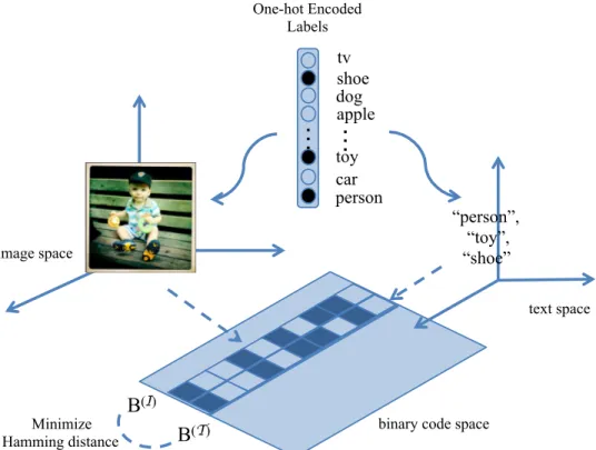
4.1 Rather than using cross-view similarities, DCVH learn discriminative view-specific binary representation via multilabel classification and align them by Hamming distance minimization via bit-wise XOR. . . 40

(15)

4.2 The overview architecture of the proposed Discriminative Cross-View Hashing (DCVH). Given multimedia data (images-texts), DCVH uses convolutional neural network (CNN) [29] to project images into binary representation; meanwhile DCVH uses pretrained GloVe [66] vectors to obtain text vector representation. Then text vectors are fed into a text-CNN [85] to generate binary representation. Unlike most methods that uses cross-view similarities, DCVH uses multilabel classification to embed raw images and texts into common binary feature space. Hammning distance minimization is adopted for view alignment purpose. . . 42

4.3 Direct Binary Embedding (DBE) layer architecture and how it is concatenated to a convolutional neural network (CNN) for images or texts. CNN(I) and CNN(T) are the corresponding CNN for images and text. DBE layer uses a linear transform and batch normalization (BN) with compound nonlinearity: rectified linear unit (ReLU) and tanh, to transform CNN activation to binary-like latent feature spaceZ(S) _{. . . .} ₄₆ 4.4 Comparison of precision-recall curve with code length of 64 bits on tasks:

image query with text dataset (I-D, T-D) and text query with image dataset (I-D, T-D), on MS COCO ((a), (b)), and MIFLICKR ((c), (d)). . . 51

4.5 Impact of λ on DCVH, evaluated on several tasks including image query retrieving from text database (I-Q, T-D); text query retrieving from image database (I-D, T-Q); image query retrieving from image database (I-I); and image annotation. mAP is used as evaluation metric for retrieval tasks and overall F1 score (O-F1) is used for annotation task. The code length is set as 64 bits across the experiments.. . . 56

(16)

5.1 The overall architecture of the proposed p-ABR. Images of source (labeled) and target (unlabeled) domains are fed into two separate nonlinear projections serving as hashing function, including CNN, fully-connected layer (FC), Direct Binary Embedding layer (DBE). In addition, a discriminator (D) is employed to determine which domain the DBE layer activation belongs to. We use 2-stage training to obtain the hashing functions for two domains. In 2-stage 1, network for the labeled domain (CNN together with FC layer and DBE layer) is trained via classification task; in stage 2, network for the unlabeled domain is updated via adversarial learning while fixing the labeled domain network. The progressive learning of binary representation is shown in the dashed box. The blue blocks are binary representations, the green blocks are the output of linear classifiers, i.e., predictions, the arrows indicate the direction along which the previous prediction is added to. Best viewed in color. . . 63

5.2 Divide the representation into column-wise blocks. . . 64

5.3 Comparison between conventional binary representation and progressive binary representation for domain adaptation. . . 75

6.1 Overview of Faster R-CNN . . . 80

6.2 The overall architecture of the proposed Det-Bit . . . 82

6.3 Comparison between Det-Bits and Faster R-CNN across code-length of 64, 128, 256, 512-bit . . . 84

(17)

Chapter 1

Introduction

(18)

Modern computer vision tasks such as smart camera networks (SCNs) [61] and

large-scale visual data mining is becoming more and more ubiquitous and demanding.

Computer vision tasks on huge collections of images and video are usually challenging due to its overwhelming size or high dimensionality, making recognition or similarity search inefficient and unaffordable. Many large-scale datasets such as ImageNet [38] have become available, enabling better studying more sophisticated algorithms. Meanwhile online sharing of user-generated content grows exponentially. For instance, Facebook has about 300 million photo uploads per day [22]. On the other hand, due to the resource-constrained nature of smart camera networks, often deployed in a distributed fashion with limited onboard processing, storage and transmission capacity, SCNs cannot handle large data transfer in typical applications like distributed object/scene recognition [Luo and Qi]. Moreover, modern media along with the large scale datasets generated by them brought forward following new challenges that traditional computer vision rarely dealt with:

1. rapidly growing social media offer massive volumes of multimedia content as well, e.g., photo posts with textual tags on Flickr, tweets with pictures, etc. It is desired to perform efficient content understanding and analytics across different media modalities.

2. Generating labels for large scale datasets is usually prohibitively expensive, and newly available datasets often do not come with label information, from which it is still desired to retrieve relevant data pertaining to labeled images. While this is achievable thanks to the transferability of deep structure [88], the non-negligible domain shift existing between different domains hinders more effective cross-domain image retrieval.

These high-demanding applications (e.g., SCNs and scalable data mining) are becoming more and more ubiquitous and renders renders it urgent to generate more efficient representations or descriptors of high fidelity for image datasets. Consequently learning high-quality binary representation is tempting due to its compactness and representation capacity.

The binary representation or image hashing, has been widely used in areas like massive data mining and large-scale machine learning, such as relevant information retrieval and similarity search [93, 27, 84, 55]. It maps high-dimensional and continuous valued data into compact binary codes, leading to considerable savings on both space (storage and

(19)

transmission) and time (computational complexity), thus becomes an ideal descriptor for representing large-scale datasets and solving resource-constrained problems in SCNs. Image hashing algorithms have been evolving from data-independent techniques [11] to data-driven methods, such as Spectral Hashing [84], Binary Reconstructive Embedding (BRE) [40], iterative quantization (ITQ) [20]. During the past decade, deep neural networks, such as autoencoder [33], restricted Boltzman machine (RBM) [74, 25] and convolutional neural network (CNN) [38,82] have enabled the generation of highly semantic-preserving features. The recently developed VGG model [2] stacked over ten convolutional layers, generating high-level features and delivering outstanding classification performance. The deep residual network [29] (ResNet) pushed the limit of deep neural networks even further, resulting in networks of hundreds or even a thousand layers. Nonetheless, the real-valued features generated by the deep models are usually high-dimensional and are still too computationally heavy in applications like SCNs. Some recent studies [42, 90] attempted to leverage the deep models and were able to generate high-quality hash code. Majority of these approaches exploited the similarity information between samples for retrieval purpose. More specifically, this is realized by characterizing the similarity in a pre-defined neighborhood. Usually pairwise or triplet similarity are considered to capture such similarity among image pairs or triplets, respectively [56, 92, 51]. Although respecting the similarity semantics of the original dataset, the uniqueness of each individual is ignored, making it difficult to use the binary code to perform tasks like classification. Therefore it is very beneficial to generate effective binary representation that can be used for not only similarity search, indexing and retrieval, but also great for recognition and classification. Recently this gap was filled by several hashing algorithms that learn binary representation via classification [87, 75, 52]. Not only does the learned binary code retrieves images effectively, it provides comparable or even superior performance for classification as well. Meanwhile, due to the discrete nature of binary code, it is usually impractical to optimize discrete hashing function directly. Most hashing approaches attempt solving it by a continuous relaxation and quantization loss [75, 51]. However, such optimization is usually not statistically stable [92] and thus leads to suboptimal hash code.

(20)

Starting with the discussion of learning binary representation via classification tasks with cross entropy, this work focuses on the learning of discriminative binary representation for image datasets. Not only is the learned binary representation suitable for retrieval purpose, it also can be used as for classification tasks and annotation purposes, enabling learning multitasking representations. In this work, we first study the merits of learning binary representation for images using discriminative information instead of conventionally used similarity information. This is realized by utilizing label information directly with cross entropy as the loss function. Then we propose a novel architecture of binary embedding in deep neural network directly, enabling end-to-end learning of binary representation. Furthermore, we study the three scenarios where binary representation can be helpful: cross-view image hashing, cross-domain image understanding, and instance-level binary representation learning. We conduct extensive experiments to evaluate the proposed algorithms. Empirical evidences suggest that the proposed methods provide superior performance across various tasks.

(21)

Chapter 2

Learning Effective Binary Descriptors

via Cross Entropy

(22)

A version of this chapter was originally published by Liu Liu and Hairong Qi:

Liu Liu, Hairong Qi, ”Learning Effective Binary Descriptors via Cross Entropy”, IEEE

Winter Conference on Applications of Computer Vision (WACV) 2017.

2.1

Abstract

Binary descriptors not only are beneficial for similarity search, they are also capable of serving as discriminant features for classification purpose. In this paper we propose a new algorithm based on cross entropy to learn effective binary descriptors, dubbed CE-Bits, providing an alternative to L-2 and hinge loss learning. Because of the usage of cross entropy, a min-max binary NP-hard problem is raised to optimize the binary code during training. We provide a novel solution by breaking the binary code into independent blocks and optimize them individually. Although suboptimal, our method converges very fast and outperforms its L-2 and hinge loss counterparts. By conducting extensive experiments on several benchmark datasets, we show that CE-Bits efficiently generates effective binary descriptors for both classification and retrieval tasks and outperforms state-of-the-art supervised hashing algorithms.

2.2

Introduction

With the emergence of modern applications like smart camera networks (SCNs) [61]

and large-scale data mining, computer vision tasks on huge collections of images and

video are usually becoming more and more challenging due to its overwhelming size or high dimensionality, making recognition or similarity search inefficient and unaffordable. Many large-scale datasets such as ImageNet [38] have become available, enabling better studying more sophisticated algorithms. Meanwhile online sharing of user-generated content grows exponentially. For instance, Facebook has about 300 million photo uploads per day [22]. On the other hand, due to the resource-constrained nature of smart camera networks, often deployed in a distributed fashion with limited onboard processing, storage and transmission capacity, SCNs cannot handle large data transfer in typical applications like distributed

(23)

object/scene recognition [Luo and Qi]. These high-demanding applications (e.g., SCNs and scalable data mining) are becoming more and more ubiquitous and renders renders it urgent to have a significantly more efficient feature descriptor of high fidelity.

The binary code or hashing techniques, has been widely used in areas like massive data mining and large-scale machine learning [93, 27, 84, 55]. It maps high-dimensional and continuous valued data into compact binary codes, leading to considerable savings on both space (storage and transmission) and time (computational complexity), thus becomes an ideal descriptor for representing large-scale datasets and solving resource-constrained problems in SCNs. Image hashing algorithms have been evolving from data-independent techniques [11] to data-driven methods, such as Spectral Hashing [84], Binary Reconstructive Embedding (BRE) [40], iterative quantization (ITQ) [20]. During the past decade, deep neural networks, such as autoencoder [33], restricted Boltzman machine (RBM) [74,25] and convolutional neural network (CNN) [38,82] have enabled the generation of highly semantic-preserving features. The recently developed VGG model [2] stacked over ten convolutional layers, generating high-level features and delivering outstanding classification performance. The deep residual network [29] (ResNet) pushed the limit of deep neural networks even further, resulting in networks of hundreds or even a thousand layers. Nonetheless, the real-valued features generated by the deep models are usually high-dimensional and are still too computationally heavy in applications like SCNs. Some recent studies [42, 90] attempted to leverage the deep models and were able to generate high-quality hash code. However, majority of these approaches exploited the similarity information between samples for retrieval purpose, ignoring the uniqueness of each individual, making it difficult to use the binary code to perform tasks like classification. Therefore it is very beneficial to generate effective binary descriptors that can be used for not only similarity search, indexing and retrieval, but also great for recognition and classification.

Albeit the success of image hashing, learning effective binary descriptors is still an open-end topic. Although several efficient binary descriptors, e.g., BRIEF [7], BRISK [44], and FREAK [64], have been proposed to describe images without label information. However they tend to be unstable and inconsistent to the image invariant. Deep learning based binary descriptor [46] has been proposed to generate high-quality binary descriptor. But

(24)

it does not generalize the situation where existing continuous-valued features are already available. In this paper, we propose a new method to generate binary representations for images, which not only enjoys the high-quality features from deep neural networks, but also can be applied to resource-constrained environment like smart camera networks, where both computation and storage resources are restricted. Inspired by classic classification paradigm, we propose to use cross entropy as the loss function. Because of the use of cross entropy, we are faced with an NP-hard combinatorial optimization problem during training. We provide a suboptimal block-by-block greedy optimization algorithm for the binary codes. Empirical studies demonstrate that our training algorithm converges very fast. Moreover, experiment results also show that our method outperforms state-of-the-art supervised hashing algorithms, including its L-2 and hinge loss counterpstate-of-the-arts, on both classification and retrieval tasks.

2.3

Learning Binary Descriptors via Classification

Demonstrated by previous studies such as [75], binary descriptors learned via classification preserve the semantic similarity and discriminative information of the original data and serve multiple purposes. Not only can they be used for classification, they are also good hash code for retrieval task. Similar to the setup in [75], the binary descriptors are learned via classification. Specifically, given a dataset ofN samplesX={xi}i=1N , xi ∈Rd×1, we aim

to learn the binary representation for the dataset, denoted by B={bi}i=1N ∈ {−1,+1}L×N,

which is obtained by taking the sign of a learned embedding function F : _Rd×N _7→

RL×N, L << d:

B= sgn(F(X)) (2.1)

Meanwhile a linear classifier is used to take the advantage of the label information associated with X, namely Y, where Y ={yi}i=1N , yi ={1, . . . , C}, i = 1, . . . , N, and C is the number

(25)

obtained by using the following optimization problem similar to [75]: min W,F 1 N N X i=1 L(WTbi, yi) + Ω(W) bi = sgn(F(xi))∈ {−1,+1}L, i= 1, . . . , N (2.2)

where L is some loss function measuring the error between the prediction and ground truth

Y during training, and Ω is the regularizor for the classifier.

Common choices for loss function are L-2 loss (dictionary learning [78] and supervised modeling [25]), hinge loss (SVM), and cross entropy (neural networks). With L-2 loss and hinge loss explored in [75], in this paper we choose to use cross entropy as the loss function as it raises a new optimization problem, leading to a more efficient solution for generating the binary descriptors as demonstrated by extensive experiments in Section 4.5. Consequently the classifier we use here issoftmax. Softmax is a generalization of binary logistic regression classifier, which tends to give a more intuitive result in a probabilistic sense. The weight of the classifier W can be expanded as {w1, . . . ,wC} where wk ∈ RL×1 is for category k.

Unnormalized probability of prediction for category k can then be expressed asewTkbi_{. And}

the normalized probability of prediction is:

P(yi =k|bi;wk) = ewT kbi PC j=1e wT jbi (2.3)

Cross entropy aims to minimize the difference of probability distribution between the predicted labels and ground truth labels. For each sample we have:

Li =− C X

k=1

tk(yi) logP(yi =k|bi;wk), (2.4)

wheretk(yi) is the distribution of ground truth labelsyi; P(yi =k|bi;wk) is the distribution

of predicted labels. This is equivalent to Kullback-Leibler divergence since the entropy of the ground truth is a constant and does not contribute, and both of which attempt to minimize the distance between two distributions. Note that the distribution of ground truth label tk can be simplified as identity function since each training sample only belongs to

(26)

one category k, i.e., PC_k=1tk(yi) = 1(yi = k), furthermore simplified as 1(yi). Substitute

Eq. 2.4 into Eq.2.2 and use Frobenius norm regularization as Ω, we formulate the following optimization problem: min bi,W,F −1 N N X i=1 1(yi) wTkbi−log C X j=1 ewTjbi ! +λkWk2_F bi = sgn(F(xi)), i= 1, . . . , N (2.5)

It is difficult to optimize Eq. 2.5 directly due to the discontinuity introduced by sgn(·). Following the relaxation in [75], we add a penalty that accounts for the deviation between the continuous embedding function F and the binary code B. Eq.2.5 is reformulated as

min bi,W,F ( − 1 N N X i=1 1(yi) wTkbi−log C X j=1 ewTjbi ! + +λkWk2 F +γ N X i=1 kbi−F(xi)k22+ρkFk 2 2 ) s.t. bi ∈ {−1,+1}L, i= 1, . . . , N. (2.6) where γ is the coefficient for the regularization of the embedding function F.

Since there are multiple sets of parameters to learn, Eq.2.6 can be solved iteratively set by set. As mentioned before, because of the usage of the cross entropy as the loss function, the problem becomes NP-hard. We share the same paradigm as outlined in [75] where the F step is the same, but the W step and B step need to be redesigned.

2.3.1

F step: embedding function optimization

Following [56,75], we use a very popular and powerful nonlinear embedding mapping function of the form

F(x) =MTφ(x) (2.7) whereM∈_Rm×L_{is a linear mapping;}_φ(_x_{) = [K}₍_x_,_x

1), K(x,x2),· · · , K(x,xm)]T. K(x,xi),

i = 1,· · · , m is a kernel function and points {xi}mi=1 are anchors uniformly sampled from

training set. A popular choice for kernel function is the RBF kernel function K(x,xi) =

(27)

In order to optimize the embedding function parameterized byM, we fix the binary code B and classifier W and we have

min M N X i=1 kbi−MTφ(xi)k22+ρkMk22 s.t. bi ={−1,+1} L . (2.8)

Eq. 2.8 can be rewritten in matrix form

min M kB−M T_φ(_X₎_k2 2+ρkMk 2 2 s.t. B ={−1,+1}L×N. (2.9)

Eq. 2.9 can be solved by the regularized least square

M= (φ(X)φ(X)T +ρI)−1φ(X)B (2.10)

2.3.2

W step: classifier optimization

By fixing binary codeBand the embedding functionF, classifier can be optimized by solving the following problem:

min W − 1 N N X i=1 1(yi) log ewTkbi PC j=1e wT jbi +λkWk 2 F, (2.11)

which can be solved through gradient based approaches. The gradient of the objective function in Eq. 2.11 with respect to each wk associated with category k is

∂L ∂wk =−1 N N X i=1 " bi 1(yi)− ewTkbi PC j=1e wT jbi !# + 2λwk (2.12)

In order to accelerate gradient descent in the relevant direction and dampen the oscillation phenomenon during learning process, momentum [67] is used. Then the updating rule for

(28)

wk is

v(t) =θv(t−1)+α ∂L ∂w_k(t−1)

w(t+1)_k =w(t)_k −v(t), ∀k = 1, . . . , C

(2.13)

where θ is the momentum term, usually set to 0.9 or smaller, α is the learning rate.

2.3.3

B step: binary code optimization

SimilarlyBis optimized by fixing WandF (defined in Eq. 5.10), and we have the following optimization problem, min bi ( − 1 N N X i=1 1(yi)wTkbi+ 2γ N X i=1 F(xi)Tbi ! + 1 N N X i=1 log C X j=1 ewTjbi ) s.t. bi ∈ {−1,1}L, i= 1, . . . , N. (2.14)

where logPC_j=1ewTjbi _{in problem (}_2.14_{) is a}_Log-Sum-Exp _{(LSE) function, which is a smooth}

approximation to the maximum function, owing to the following tight bounds,

max{x1, . . . , xn} ≤LSE(x1, . . . , xn)≤max{x1, . . . , xn}+ log(n) (2.15)

When {xi}n1 are large enough, LSE can be approximated directly by the maximum function.

Here even ifxi =wTkbi is not large enough, we can still accomplish the approximation since

LSE(wT

kbi) =−m+ logPN_i=1exp(wTkbi +m), wherem is a large enough number. In fact,

many use such trick to prevent numerical overflow of calculating LSE(xn) in practice and

ususally m= maxn(xn) in such case.

As a result, Eq. 2.14 can be approximated as

min bi ( − 1 N N X i=1 1(yi)wTkbi+ 2γ N X i=1 F(xi)Tbi ! + 1 N N X i=1 max j {w T j bi} ) s.t. bi ∈ {−1,+1}L, i= 1, . . . , N. (2.16)

Clearly Eq.2.16is an NP-hard combinatorial problem. We choose to solvebiby exhaustively

(29)

is O(2N L_{). Usually it is impossible to solve the problem if we directly search the whole}

solution space. The following two observations inspire our suboptimal solution. The input images can be considered as independent samples (i.i.d for each category); meanwhile each bit of the binary code can be treated as a random variable following the same Bernoulli

distribution, and we assume the bits are statistically independent. As a matter of fact, we

can exchange the order of the sum and minimization of Eq. 2.16

N X i=1 min bi − 1 N1(yi)w T kbi+ 2γF(xi)Tbi + 1 N maxj {w T jbi} s.t. bi ∈ {−1,1}L, i= 1, . . . , N. (2.17)

So the binary hash code for each sample can be optimized independently. Denoting the optimization problem2.17forith sample’s binary codebi asJ(bi), by ”divide and conquer”,

we can solve J(bi) in a greedy way. To see this, we decompose the problem into two

sub-problems by splitting the binary code bi into two halvesbi,1 and bi,2:

min bi J(bi) = min bi,1,bi,2 − 1 N 1(yi)w T k,1bi,1+1(yi)wk,2T bi,2 −2γ F1(xi)Tbi,1+F2(xi)Tbi,2 +1 N maxj {w T j,1bi,1+wj,2T bi,2} ≈ min bi,1,bi,2 −1 N 1(yi)w T k,1bi,1 +1(yi)wTk,2bi,2 −2γ F1(xi)Tbi,1+F2(xi)Tbi,2 +1 N maxj {w T j,1bi,1}+ 1 N max{w T j,2bi,2} = min bi,1 J(bi,1) + min bi,2 J(bi,2) (2.18)

Now we have two separate optimization problems with the identical form. And this splitting process continues until solving the sub-problem by exhaustive search is affordable. The process is shown in Fig. 5.2. More specifically, the pth block of the ith sample can be optimized by J(b(i,p)), which can be solved in O(logC + 2L0) due to finding maximum

of WT

(p,:)b(i,p), where L0 is the size of a block. We can choose an affordable L0 as the

(30)

complexity O(2L0_N ·L

L0

logC), equivalent to O(N LlogC) since L0 is a constant. Despite

the suboptimality of the solution, it provides an efficient, yet still effective approach to tackle the NP-hard problem. Empirically we set L0 to 4, providing both high performance

and efficient training.

Figure 2.1: The procedure of decomposition of the problem using dynamic programming.

The L-bit long optimization problem J(bi) can be decomposed into bit-wise optimization

problem J(b(i,j)), sharing exactly the same formulation of the original problem

The proposed CE-Bits is summarized in Algorithm 1.

2.4

Experiments

We evaluate the proposed CE-Bits on three challenging datasets: CIFAR-10, the Berkeley multiview wireless (BMW) and the Oxford 17 category flowers [62]. CIFAR-10 serves as a large dataset benchmark while BMW and Oxford 17 category flowers datasets are used in the smart camera network scenario. On each dataset we compare our algorithm with state-of-the-art supervised hashing algorithms (KSH [56], FasthHash [45], SDH [75], CCA-ITQ [20]) and provide extensive experiments on image classification task as well as image retrieval task. For the classification task, we split each dataset into a training set, and a testing set. In order to select an appropriate set of parameters for CE-Bits, we further randomly select a small set as the validation set. The performance of the classification task is evaluated by

(31)

Algorithm 1 Cross Entropy Hashing Classification

Input: Training set {X,Y}; code width L; number of iterations R; learning rate α;

parameterλ,ν.

Output: Classifier weight W; binary hash code matrixB; hash functionF(·); prediction

of classification

Step 1: Initialization

initialize W, B randomly; randomly pick anchors from training set; store solution spaceb0 = [−1,+1]T for exhaustive search; initialize F(x)

while i < R do i=i+ 1 (B Step) for j = 1, . . . , N do for k = 1, . . . , L do m1 ←maxc{wTcbbase/N} m2 ←(WT_(k,_Y_(j))/N +γ∗F(x)j,k)b0 Bj,k ←arg min−1,+1{m1+m2} end for end for (G Step) vt=θvt−1+α_∂∂_wL k wk=wk−vt, ∀k = 1, . . . , C (F Step) P←(φ(X)φ(X)T₎−1_φ(_X₎_BT end while

(32)

the accuracy on the testing set. Based on the model trained by the classification task, the retrieval task treats testing set as the query set and training set as the retrieval database. The performance of the retrieval task is evaluated by the mean average precision (MAP). In the experiments we use the recommended parameters for the compared algorithms.

2.4.1

Datasets

The CIFAR-10 dataset consists of 60,000 color images in 10 classes. Each class has 6,000 images in size 32× 32. We randomly select 50,000 samples as the training set and the rest 10,000 as the testing set. And a validation set is split by randomly selecting 5,000 samples from the training set. Due to recent huge success achieved by deep neural network on large datasets like CIFAR-10, we represent the dataset using the output from the finally fully-connected layer of a 50-layer deep residual network, which is specifically trained on CIFAR-10. Each sample is a 64-dimension floating number vector.

The BMW dataset contains 20 landmark buildings on the campus of the University of California, Berkeley. 16 different vantage points are selected for each building to capture the 3-D appearance of the building. At each vantage point 5 short-baseline images are taken by 5 cameras simultaneously, leading to 80 images per category. And each image is a 640×480 RGB color image. For the experiments, we use images captured by camera #2 (320 images) as the training dataset (a validation set of 4 randomly selected samples per class is used for parameter selection), and rest images are testing dataset. Each image is described by a 500-dimension bag-of-words SURF [5] features.

The Oxford 17 category flower dataset [62] contains images of 17 categories of flowers. There are totally 1,380 images with each class consists of 80 images. A training set with 40 images per class, a validation set with 20 images per class and a testing set with 20 images per class are split. Instead of using the raw pixels (227×227×3), we use the pre-trained VGG model [2] (trained on the ImageNet dataset [12]) and obtain a 4096-dimension floating number vector for each image.

(33)

2.4.2

Classification Task

Here we provide the comparison of testing accuracy on three datasets. In order to make a fair comparison, liblinear [15] is used as the classifier to assess the quality of the binary codes on classification task. Results with 64 bits are reported across all the methods. We also report the training time of the algorithms to compare the efficiency. Table 3.3, 2.2,

2.3 shows the results on CIFAR-10, Oxford 17 category flower [62] and BMW respectively. Note that due to fact that KSH requires huge memory and long time to train, a 5,000-sample training subset is randomly selected from the original 50,000-sample training set. To provide fair comparison, we also provide the result of CE-Bits that is trained on the same subset.

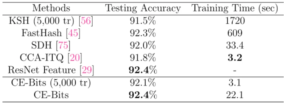
Table 2.1: The testing accuracy of different methods on CIFAR-10 dataset (ResNet

features), all binary codes are 64 bits.

Methods Testing Accuracy Training Time (sec) KSH (5,000 tr) [56] 91.5% 1720 FastHash [45] 92.3% 609 SDH [75] 92.0% 33.4 CCA-ITQ [20] 91.8% 3.2 ResNet Feature [29] 92.4% -CE-Bits (5,000 tr) 92.1% 3.1 CE-Bits 92.4% 22.1

Table 2.2: The testing accuracy of different methods on Oxford 17 category flower

dataset [62] (VGG features), all binary codes are 64 bits.

Methods Testing Accuracy Training Time (sec) KSH [56] 87.4% 83.1 FastHash [45] 88.5% 38.0 SDH [75] 87.9% 0.71 CCA-ITQ [20] 88.5% 7.67 VGG Feature [2] 88.8% -CE-Bits 88.6% 1.12

For all three challenging datasets, CE-Bits achieves the best accuracy among all the state-of-the-art supervised hashing algorithms. We can conclude that CE-Bits preserves

(34)

Table 2.3: The testing accuracy of different methods on BMW dataset (SURF features), all binary codes are 64 bits.

Methods Testing Accuracy Training Time (sec) KSH [56] 93.8% 18.4 FastHash [45] 91.1% 14.8 SDH [75] 95.9% 0.15 CCA-ITQ [20] 92.9% 1.17 SURF [5] 94.7% -CE-Bits 97.2% 0.31

the discriminant information of the original floating-number data. For CIFAR-10 dataset, CE-Bits achieves the same best accuracy as the floating-number residual network features with a very low training time. Not only does this demonstrates that CE-Bits preserves the semantics of the ResNet features, it also implies the significant level of redundancy in the original floating-number features. Despite the fact that CCA-ITQ uses the least time to train the model, the testing accuracy is lower than CE-Bits. In addition, CCA-ITQ is sensitive to the dimension of the input, i.e., it achieves the lowest training time solely because the residual network feature of CIFAR-10 is only 64-dimension.

For Oxford 17 category flower dataset [62], CE-Bits delivers the best binary code classification accuracy with a very low training time with much less data, and the result is only slightly lower (0.2% lower) than the VGG [2] feature, which is 4096-dimension floating number. Similarly for BMW dataset, CE-Bits uses very low training time and achieves the best binary code classification accuracy. Note that the accuracy achieved by CE-Bits is even better than the original floating-number feature, also reported in [75], indicating that CE-Bits can extract more discriminant information. This is because the embedding function F maps the original feature to a nonlinear yet simpler feature space, enabling a high-quality binary descriptor.

2.4.3

Retrieval Task

We use CIFAR-10 as the benchmark dataset to evaluate the retrieval performance as it is usually much more challenging to do retrieval on large dataset like CIFAR-10. More

(35)

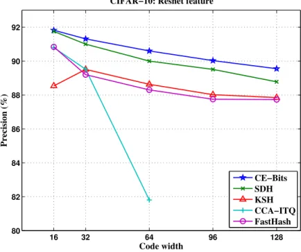
specifically, precision and mean average precision (MAP) within Hamming radius of 2 are used to evaluate the retrieval performance. Fig. 2.2 shows the comparison on precision of different methods. Based on the precision comparison, CE-Bits outperforms other state-of-the-art methods slightly across all code widths. Note that code width of CCA-ITQ is bound by the deep residual network feature of CIFAR-10, which is 64-dimension.

16 32 64 96 128 80 82 84 86 88 90 92 Code width Precision (%)

CIFAR−10: Resnet feature

CE−Bits SDH KSH CCA−ITQ FastHash

Figure 2.2: Comparison of precision achieved by different methods within Hamming radius

of 2.

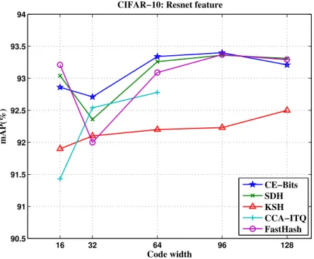
The comparison on MAP is demonstrated in Fig. 2.3. CE-Bits performs consistently well across all code widths in terms of MAP and it provides comparable results comparing to other state-of-the-art methods.

Note that we use different approaches (SURF, VGG, and ResNet) to generate features for the purpose of showing that CE-Bits can learn high-quality binary code consistently. If we use ResNet for all three datasets, CE-bits outperforms state-of-the-art algorithms as well. For Oxford 17 category flowers dataset, CE-Bits achieves classification accuracy of 94.76% and MAP of 95.47%, outperforming SDH (accuracy 93.26%, and MAP 94.59%). For BMW dataset, CE-Bits achieves accuracy of 98.02% and MAP of 99.26%, improving SDH (accuracy 97.96%, and MAP 98.57%).

(36)

16 32 64 96 128 90.5 91 91.5 92 92.5 93 93.5 94 Code width mAP(%)

CIFAR−10: Resnet feature

CE−Bits SDH KSH CCA−ITQ FastHash

Figure 2.3: Comparison of MAP achieved by different methods within Hamming radius of

2.

2.4.4

Discussion

The behavior of the proposed CE-Bits is analyzed.

Suboptimality

We use CIFAR-10 as our benchmark dataset. Since the binary code B is optimized by breaking down into smaller blocks and optimizing them independently, obviously the solution is suboptimal, and the block sizeL0 has a great impact on the effectiveness and the efficiency

of the algorithm. On one hand, the greater L0 is the closer the solution approaches to the

optimal; on the other hand, larger L0 can lead to substantially longer training time because

the complexity of exhaustive search is proportional to 2L0_{. Tab.} _2.4 _{summarizes how} _L

0

effects the algorithm. Surprisingly with smaller L0, e.g., 1-bit and 2-bit, the training time is

longer than L0 =4-bit. This is because the exhaustive search has to loop through _LL₀ blocks,

(37)

Table 2.4: Evaluation of suboptimality on different block sizeL0. The code width is 64-bit.

L0 1-bit 2-bit 4-bit 8-bit 16-bit

Testing accuracy (%) 91.5 92.0 92.4 92.3 92.4 Training Time (sec) 81 50.2 22.1 30.1 1105

Empirical Convergence

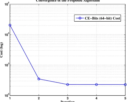
In the training stage, the derivation of embedding function has a closed form; and solving binary code is done by exhaustive search. The only factor that would affect the convergence is learning the classifier weight W. However with carefully chosen learning rate α, CE-Bits converges fast and usually it only needs fewer than 5 iterations to converge. Fig. 2.4 shows that the convergence of CE-Bits on CIFAR-10 dataset is very fast. The learning rate for CIFAR-10 isα = 5e−3, and for BMW as well as Oxford 17 category flower isα= 5e−2.

1 2 3 4 5 102 103 104 105 Iteration Cost (log)

Convergence of the Proposed Algorithm

CE−Bits (64−bit) Cost

Figure 2.4: The convergence of CE-Bits on CIFAR-10 during training with learning rate

(38)

Anchors

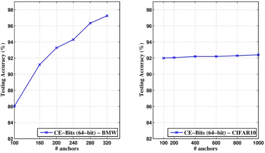
By using randomly selected anchors, the dataset is projected to a nonlinear space by the embedding function. Although the impact of the number of anchors has been discussed in previous studies [56, 75], we demonstrate that this impact is actually data-related. Fig. 2.5

displays the impact of the number of anchors on BMW dataset and CIFAR-10. For BMW dataset, increasing the number of anchors significantly improves the performance of the algorithm; while the performance on CIFAR-10 is more consistent over different number of anchors since the residual network feature is more informative and robust comparing to the traditional hand-crafted features like GIST or SURF feature.

100 160 200 240 280 320 82 84 86 88 90 92 94 96 98 # anchors Testing Accuracy (%) CE−Bits (64−bit) − BMW 100 200 400 600 800 1000 82 84 86 88 90 92 94 96 98 # anchors Testing Accuracy (%)

CE−Bits (64−bit) − CIFAR10

Figure 2.5: The testing accuracy of CE-Bits (64-bit) on BMW and CIFAR-10 regarding

various number of anchors

Benefits from Binary Codes

Clearly using binary codes to represent images saves tremendous storing space and data transmission. For instance, storing and transmitting the data for BMW dataset on smart camera sensors with the SURF feature requires about 2K Bytes for each image; while it only needs 64 bits using binary codes, only 0.4% of original space to store or transmit the data. The storage required by the binary descriptors for Oxford 17 category flower dataset [62]

(39)

is even smaller, only 0.05% of the original VGG [2] feature. Meanwhile, because of the simplicity of binary codes, the computational cost is reduced drastically too. Take CIFIAR-10 dataset for example, using linear-SVM to train and test on the original residual network dataset takes 6.617 sec while it only takes 0.0069 sec on binary codes, yielding 1,000x faster calculation.

2.5

Conclusion

In this study, we proposed a new algorithm, dubbed CE-Bits, for generating effective binary descriptor, especially for computer vision task in extreme context. Based on classic formulation of classification, our algorithm is straightforward conceptually. Cross entropy is chosen as the criterion to formulate the optimization problem. We were able to show the compact binary descriptors can be generated effectively and efficiently by extensive experiments on three challenging experiments, CIFAR-10, Oxford 17 category flower, and Berkeley multiview wireless dataset. CE-Bits outperformed other state-of-the-art algorithms consistently for handcrafted features (SURF) and deep features (VGG and ResNet), while it required less training time especially on larger datasets.

(40)

Chapter 3

End-to-end Binary Representation

Learning via Direct Binary

(41)

A version of this chapter was originally published by Liu Liu, Alireza Rahimpour, Ali Taalimi, Hairong Qi:

Liu Liu, Alireza Rahimpour, Ali Taalimi, Hairong Qi, ”End-to-end Binary Represen-tation Learning via Direct Binary Embedding”, IEEE International Conference on Image

Processing (ICIP) 2017

3.1

Abstract

Learning binary representation is essential to large-scale computer vision tasks. Most existing algorithms require a separate quantization constraint to learn effective hashing functions. In this work, we present Direct Binary Embedding (DBE), a simple yet very effective algorithm to learn binary representation in an end-to-end fashion. By appending an ingeniously designed DBE layer to the deep convolutional neural network (DCNN), DBE learns binary code directly from the continuous DBE layer activation without quantization error. By employing the deep residual network (ResNet) as DCNN component, DBE captures rich semantics from images. Furthermore, in the effort of handling multilabel images, we design a joint cross entropy loss that includes both softmax cross entropy and weighted binary cross entropy in consideration of the correlation and independence of labels, respectively. Extensive experiments demonstrate the significant superiority of DBE over state-of-the-art methods on tasks of natural object recognition, image retrieval and image annotation.

3.2

Introduction

Representation learning is key to computer vision tasks. Recently with the explosion of data availability, it is crucial for the representation to be computationally efficient as well [75,

52, 68]. Consequently learning high-quality binary representation is tempting due to its compactness and representation capacity.

Binary representation traditionally has been learned for image retrieval and similarity search purposes (image hashing). From the early works using hand-crafted visual features [20,

84, 56, 45] to recent end-to-end approaches [92, 51, 87] that take advantages of deep convolutional neural networks (DCNN), the core of image hashing is learning binary

(42)

code for images by characterizing the similarity in a pre-defined neighborhood. Usually pairwise or triplet similarity are considered to capture such similarity among image pairs or triplets, respectively [56, 92, 51]. Albeit the high-quality of binary code, most image hashing algorithms do not consider learning discriminative binary representation. Recently this gap was filled by several hashing algorithms that learn binary representation via classification [87,75,52]. Not only does the learned binary code retrieves images effectively, it provides comparable or even superior performance for classification as well. Meanwhile, due to the discrete nature of binary code, it is usually impractical to optimize discrete hashing function directly. Most hashing approaches attempt solving it by a continuous relaxation and quantization loss [75, 51]. However, such optimization is usually not statistically stable [92] and thus leads to suboptimal hash code.

In this work, we propose to learn high-quality binary representation directly from deep convolutional neural networks (DCNNs). By appending a binary embedding layer directly into the state-of-the-art DCNN, deep residual network, we train the whole network as a hashing function via classification task in attempt to learning representation that approximates binary code without the need of using quantization error. Thus we name our approach Direct Binary Embedding (DBE). Furthermore, in order to learn high-quality binary representation for multilabel images, we propose a joint cross entropy that incorporates softmax cross entropy and weighted binary sigmoid cross entropy in consideration of the correlation and independence of labels, respectively. Extensive experiments on two large-scale datasets (CIFAR-10 and Microsoft COCO) show that the proposed DBE outperforms state-of-the-art hashing algorithms on object classification and retrieval tasks. Additionally, DBE provides a comparable performance on multilabel image annotation tasks where usually continuous representation is used.

3.3

Direct Binary Embedding

3.3.1

Direct Binary Embedding (DBE) Layer

We start the discussion of DBE layer by revisiting learning binary representation using classification. Let I = {Ii}Ni=1 be the image set with n samples, associated with label set

(43)

Y = {yi}Ni=1. We aim to learn binary representation B = {bi}Ni=1 ∈ {0,+1}N

×L _of _I _via

the Direct Binary Embedding layer that is appended to DCNN. Following the paradigm of classification problem formulation in DCNN, we use a linear classifier W to classify the binary representation: min W,F 1 N N X i=1 L(W>bi, yi) +λkbi−F(Ii; Ω)k22 (3.1) s.t.bi =thresold(F(Ii; Ω),0.5)

whereL is an appropriate loss function; kbi−F(Ii; Ω)k22 measures the quantization error of

between the DCNN activationF(Ii; Ω) and the binary codebi;λis the coefficient controlling

the quantization error; threshold(v, t) is a thresholding function at t, and it equals to 1 if v ≥t, 0 otherwise; F is a composition ofn+ 1 non-linear projection functions parameterized by Ω:

F(I,Ω) =fDBE(fn(· · ·f2(f1(I;ω1);ω2)· · · ;ωn)ωDBE), (3.2)

where the innernnonlinear projections composition denotes then-layer DCNN;fDBE(·;ωDBE)

is the Direct Binary Embedding layer appended to the DCNN. The binary codebi in Eq.3.1

makes it difficult to optimize via regular DCNN inference. We relax Eq.3.1 to the following form where stochastic gradient descent is feasible:

min W,F 1 N N X i=1 L(W>F(Ii; Ω), yi) +λ||2F(Ii; Ω)−1| −1|2 (3.3)

As proved by [92], the quantization loss ||2F(Ii; Ω)−1| −1|2 in Eq. 3.3 is an upper bound

of that in Eq.3.1, making Eq. 3.3 an appropriate relaxation and much easier to optimize. Several studies such as [92] share the similar idea of encouraging the fully-connected layer representation to be binary codes by using hyperbolic tangent (tanh) activation. Since it is desirable to learn binary code B = {0,+1}N×L_{, we propose to concatenate the ReLU}

(44)

(shown in Figure 3.1):

Z =fDBE(X) = tanh(ReLU(BN(XWDBE+bDBE))) (3.4)

where X = fn(· · ·f2(f1(I;ω1);ω2)· · · ;ωn) ∈ RN×d is the activation of n-layer DCNN;

I

DCNN

W

DBE

b

_DBE

BN

tanh(ReLU(



))

X

T

Z

F

(I;

Ω

)

f

_DBE

Figure 3.1: The framework of DBE and outputs of different projections

Z =fDBE(X)∈ RN×L is the binary-like activation of DBE layer; T= BN(XWDBE+bDBE)

is the activation after linear projection and batch normalization but prior to ReLU and tanh;

WDBE ∈Rd×L is a linear projection,bDBE is the bias; BN(·) is the batch normalization. And

its activation is plotted in Figure3.2a. The benefit of DBE layer approximating binary code is three-fold:

1. batch normalization mitigates training with saturating nonlinearity such as tanh [31], and potentially promotes more effective binary representation.

2. ReLU activation is sparse [18] and learns bit ‘0’ inherently.

3. tanh activation bounds the ramping of ReLU activation and learns bit ‘1’ effectively without jeopardizing the sparsity of ReLU.

Furthermore, DBE layer learns activation that approximates binary code statistically well. Consider random sampling t from T, and assume it follows a distribution denoted by pT(t). Consequently the distribution of the DBE layer activationz =fDBE(t), and it follows

distribution pZ(z), written as:

pZ(z) = pT(fDBE−1 (z)) 1 f0 DBE(f −1 DBE(z)) (3.5)

(45)

−2 −1 0 1 2 3 4 −0.5 0 0.5 1 1.5 tanh(ReLU(t)) (a) activation 0 0.1 0.2 0.3 0.4 0.5 0.6 0.7 0.8 0.9 1 0 10 20 30 40 50 60 1/(1−t2)

(b) The PDF for positive input

Figure 3.2: tanh(ReLU(·)) activation and its PDF for positive input

Eq. 3.5 holds since fDBE is a monotonic and differentiable function. Since it is also positive

when z is positive, thus we have:

pZ(z) =pX(fDBE−1 (z))

1

1−f_DBE−1 (z)2, f

−1

DBE(z) =t >0. (3.6)

pT(fDBE−1 (z)) in Eq. 3.6 is equivalent to pT(t); ₁₋_f−11 DBE(z)2

grows sharply towards the discrete value {+1} for any positive response z, as is plotted in Figure 3.2b. This suggests that the DBE layer enforces that the learned embeddingzare assigned to{+1}with large probability as long as z is positive. Conclusively DBE layer fDBE can effectively approximate binary

code. Eventually we choose to optimize Eq. 3.3 without the quantization error and replace the binary code bi with DBE layer activation directly. Eq. 3.3 can thus be rewritten as:

min W,F 1 N N X i=1 L(W>F(Ii; Ω), yi) (3.7) s.t.F(I,Ω) =fDBE(fn(· · ·f2(f1(I;ω1);ω2)· · · ;ωn)ωDBE)

The inference of DBE is the same as canonical DCNN models via stochastic gradient descent (SGD).

(46)

3.3.2

Multiclass Image Classification

Majority of DCNNs are trained via multiclass classification using softmax cross entropy as the loss function. Following this paradigm, Eq. 3.7 can be instantiated as:

min W,F − 1 N N X i=1 C X k=1 1(yi) log ew>_kF(Ii;Ω) PC j=1e w_j>F(Ii;Ω) (3.8) s.t.F(I,Ω) =fDBE(fn(· · ·f2(f1(I;ω1);ω2)· · · ;ωn)ωDBE)

whereCis the number of categories;W= [w1, . . . ,wC] andwk, k = 1, . . . , Cis the weight of

the classifier for categoryk;yi is the label for image sampleI, and1(yi) an indicator function

representing the probability distribution for label yi. Essentially Eq. 3.8 aims to minimize

the difference between the probability distribution of ground truth label and prediction.

3.3.3

Multilabel Image Classification

More often a real-world image is associated with multiple objects belonging to different categories. A natural formulation of optimization problem for multilabel classification is extending the multiclass softmax cross entropy in Eq.3.8to multilabel cross entropy. Indeed softmax cross entropy captures the co-occurrence dependencies among labels, one cannot ignore the independence of each individual labels. For instance, ‘fork’ and ‘spoon’ usually co-exist in an image as they are associated with super-concept ‘dining’. But occasionally a ‘laptop’ can be placed randomly on the dining table where there are also ‘fork’ and ‘spoon’ in the image as well. Consequently, we propose to optimize a joint cross entropy by incorporating weighted binary sigmoid cross entropy, which models each label independently, to softmax cross entropy. Eq. 3.7 can therefore be instantiated as:

min W,F − 1 N N X i=1 c+ X j=1 1 c+ log e w_j>F(Ii;Ω) PC p=1e w> pF(Ii;Ω) −ν 1 N N X i=1 C X p=1 ρ₁(yi) log 1 1 +ew>pF(Ii;Ω) (3.9) +(1−₁(yi)) log ew>pF(Ii;Ω) 1 +ew> pF(Ii;Ω) # s.t. F(I; Ω) =fDBE(fn(· · ·f2(f1(I;ω1);ω2)· · · ;ωn)ωDBE)

(47)

where c+ is the number of positive labels for each image; ν is the coefficient controlling the

numerical balance between softmax cross entropy and binary sigmoid cross entropy; ρis the coefficient penalizing the loss for predicting positive labels incorrectly.

3.3.4

Toy Example: LeNet with MNIST Dataset

In order to demonstrate the effectiveness of DBE layer, we use LeNet as a simple example of DCNN. We add DBE layer to the last fully connected layer of LeNet and learn binary representation for MNIST dataset. MNIST dataset [43] contains 70K hand-written digits of 28×28 pixel size, ranging from ‘0’ to ‘9’. The dataset is split into a 60K training set (including a 5K validation set) and a 10K test set1. We enhance the original LeNet with more convolutional kernels (16 kernels and 32 kernels on the first and second layer, respectively, all with size 3×3). We train the LeNet with DBE layer on the training set and evaluate the quality of learned binary representation on the test set. Figure 3.3a demonstrates the histogram of activation from DBE. Clearly DBE layer learns a representation approximating binary code effectively (51.1% of DBE activation less than 0.01, 48.6% greater than 0.99 and only 0.3% in between). We evaluate the quality of binary code learned by DBE qualitatively by comparing the classification accuracy on the test set with the state-of-the-art hashing algorithm. In order to demonstrate the effectiveness of DBE, we also compare with different λ in Eq.3.3 for the purpose of showing that quantization error is not necessary anymore to learn high-quality binary representation. From Table 3.2 we can see that with the increase of λ in Eq. 3.3, the testing accuracy decreases. Due to the effectiveness of DBE layer, quantization error does not contribute to the binary code learning. Following the evaluation protocol of previous works [75], linear-SVM [15] is used as the classifier on all compared methods for fair comparison (including continuous LeNet representation). The classification accuracy on the test set is reported in Table 3.1.

The convergence of training DBE-LeNet is reported in Figure3.3b. Due to the saturating tanh activation, the gradient is slightly more difficult to propagate through the network. Eventually the convergence reaches the same level.

(48)

(a) 0 10 20 30 40 50 60 70 80 epcohs 10-3 10-2 10-1 100 101 log(Loss) DBE-LeNet LeNet (b)

Figure 3.3: The qualitatively results of DBE-LeNet: (a)The histogram of DBE layer

activation; (b)The convergence of the original LeNet and with DBE trained on MNIST

Table 3.1: The comparison of the testing accuracy on MNIST. Code-length for all hashing

algorithms is 64-bit. LeNet feature (1000-d continuous vectors) is used for SDH and FastHash.

Method LeNet [43] DBE-LeNet SDH [75] FastHash [45] testing acc(%) 99.34 99.34 99.14 98.62

Table 3.2: The impact on quantization error coefficient λ

λ 0 1e-4 1e-3 1e-2 1e-1 testing acc(%) 99.34 99.34 99.30 99.26 99.01

3.4

Experiments

We evaluate the proposed DBE layer with the deep residual network (ResNet). We choose to append DBE layer to the state-of-the-art DCNN, 50-layer Residual Network (ResNet-50) [29] to learn high-quality binary representation for image sets. For the multilabel experiments, we set ν = 2 andρ = 5 through extensive empirical study.

3.4.1

Dataset

CIFAR-10dataset [37] contains 60K color images (size 32×32) with each image containing

a natural object. There are 10 categories of objects in total, with each category containing 6K images. The dataset is randomly split into a 50K training set and a 10K testing set. For

(49)

traditional image hashing algorithms, we provide 512-D GIST [63] feature; for end-to-end deep hashing algorithms, we use raw images as input directly. Microsoft COCO 2014

(COCO) [48] is a dataset for image recognition, segmentation and captioning. It contains

a training set of 83K images with 605K annotations and a validation set of 40K images with 292K annotations. There are totally 80 categories of annotations. We treat annotations as labels for images. On average each image contains 7.3 labels. Since images in COCO are color images with various sizes, we resize them to 224×224.

3.4.2

Object Classification

To evaluate the capability of mulitclass object classification, we compare DBE with several state-of-the-art supervised approaches including FastHash [45], SDH [75], CCA-ITQ [20] and deep method DLBHC [47]. The ResNet-50 features are also included in the comparison. The code-length of binary code from all the hashing methods is 64 bits. We use linear-SVM to evaluate the all the approaches on the classification task.

Table 3.3 shows the classification accuracy on test sets for the two datasets. The accuracy achieved by DBE matches that of the original continuous ResNet-50 features. DBE improves the state-of-the-art traditional methods and end-to-end approaches by 28.6% and 5.6%, respectively. And it achieves the same performance as that of the original ResNet. This demonstrates 1) DBE’s superior capability of preserving the rich semantic information extracted by ResNet, 2) there exists great redundancy in the original ResNet features.

Table 3.3: The testing accuracy of different methods on CIFAR-10 dataset. All binary

representations have code-length of 64 bits.

Methods Testing Accuracy (%) CCA-ITQ [20] 56.34 FastHash [45] 57.82 SDH [75] 67.73 DLBHC [47] 86.73 ResNet [29] 92.38 DBE (ours) 92.35

(50)

Furthermore we also provide the classification accuracy on CIFAR-10 with respect to different code lengths in Table 3.4. From the table we can conclude that DBE learns high-quality binary representation consistently.

Table 3.4: Classification accuracy of DBE on CIFAR-10 dataset across different code

lengths

Code length (bits) 16 32 48 64 128 testing acc(%) 91.63 92.04 92.20 92.35 92.36

3.4.3

Image Retrieval

Natural Object Retrieval

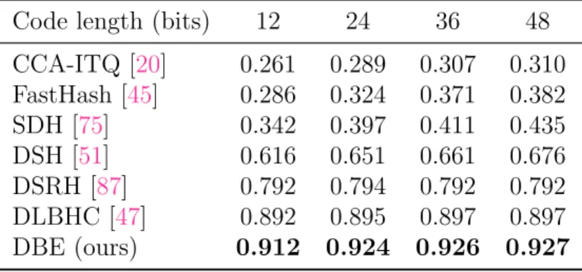
The CIFAR-10 dataset is used to evaluate the proposed DBE on natural object retrieval task. We choose to compare with state-of-the-art image hashing algorithms including both traditional hashing methods: CCA-ITQ [20], FastHash [45], and end-to-end deep hashing methods: DSH [51], DSRH [87]. For the experimental settings, we randomly select 100 images per category and obtain a query set with 1K images. Mean average precision (mAP) is used as the evaluation metric. The comparison is reported in Table3.5. The proposed DBE outperforms state-of-the-art by around 3%. It confirms that DBE is capable of preserving rich semantics extracted by the ResNet from original images and learning high-quality binary code for retrieval purpose.

Table 3.5: Comparison of mean average precision (mAP) on CIFAR-10

Code length (bits) 12 24 36 48 CCA-ITQ [20] 0.261 0.289 0.307 0.310 FastHash [45] 0.286 0.324 0.371 0.382 SDH [75] 0.342 0.397 0.411 0.435 DSH [51] 0.616 0.651 0.661 0.676 DSRH [87] 0.792 0.794 0.792 0.792 DLBHC [47] 0.892 0.895 0.897 0.897 DBE (ours) 0.912 0.924 0.926 0.927

(51)

Multilabel Image Retrieval

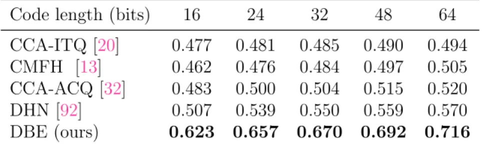
COCO dataset is used for multilabel image retrieval task. Considering the large number of labels in COCO, we compare DBE with several cross modal hashing and quantization algorithms. Studies have shown that cross-modal hashing improves unimodal methods by leveraging semantic information of text/label modality [69, 32]. We choose to compare with CMFH [13] and CCA-ACQ [32]. Furthermore we also include traditional hashing method CCA-ITQ [20] and end-to-end approach DHN [92]. Following the experiment protocols in [32], 1000 images are randomly sampled from validation set for query and the training set is used for database for retrieval. And AlexNet [39] feature is used as input for algorithms that are not end-to-end, and raw images are used for end-to-end deep hashing algorithms. Due to the multilabel nature of COCO, we consider the true neighbors of a query image as the retrieved images sharing at least one labels with the query. Similar to natural object retrieval, mean average precision (mAP) is used as evaluation metric.

Table 3.6: Comparison of mean average precision (mAP) on COCO.

Code length (bits) 16 24 32 48 64 CCA-ITQ [20] 0.477 0.481 0.485 0.490 0.494 CMFH [13] 0.462 0.476 0.484 0.497 0.505 CCA-ACQ [32] 0.483 0.500 0.504 0.515 0.520 DHN [92] 0.507 0.539 0.550 0.559 0.570 DBE (ours) 0.623 0.657 0.670 0.692 0.716

3.4.4

Multilabel Image Annotation

We generate prediction of labels for each image in validation set based onK highest ranked labels and compare to the ground truth labels. The overall precision (O-P), recall (O-C), and F1-score (O-F1) of the prediction are used as evaluation metrics. Formally they are defined as:

O-P = NCP NP

, O-R = NCP NG

, O-F1 = 2 O-P·O-R

(52)

where C is the number of annotations/labels; NCP is the number of correctly predicted

labels for validation set;NP is the total number of predicted labels; NG is the total number

of ground truth labels for validation set.

We compare DBE with softmax, binary cross entropy and WARP [19], one of the state-of-the-art for multilabel image annotation. The performance comparison is summarized in Table 4.3 and we set K = 3 in the experiment. It can be observed that the binary representation learned by DBE achieves the best performance in terms of overall-F1 score. Due to its consideration of co-occurrence and independence of labels, DBE-joint cross entropy outperforms DBE-softmax and DBE-weighted binary cross entropy.

Table 3.7: Performance comparison on COCO forK = 3. The code length for all the DBE

methods is 64-bit.

Method O-P O-R O-F1

WARP [19] 59.8 61.4 60.6 DBE-Softmax 59.1 62.1 60.3 DBE-weighted binary cross entropy 57.1 60.8 58.9 DBE-joint cross entropy 59.5 62.7 61.1

3.4.5

The Impact of DCNN Structure

Similar to most deep hashing algorithms, DBE also preserves semantics from DCNN. Consequently the structure of DCNNs influences the quality of binary code significantly. We compare with the state-of-the-art DLBHC [47] and the DCNN it uses: AlexNet [39], which the upper bound in this comparison. Since DLBHC uses AlexNet, we also use AlexNet in our DBE. CIFAR-10 dataset is used. According to results reported in Table 3.8, DBE achieves higher accuracy than DLBHC