Bootstrap confidence bands and partial linear quantile regression

(1)

Contents lists available atSciVerse ScienceDirect

Journal of Multivariate Analysis

journal homepage:www.elsevier.com/locate/jmva

✩

Song Song

a,b,∗

, Ya’acov Ritov

c

, Wolfgang K. Härdle

a

a_{Humboldt-Universität zu Berlin, Germany} b_{The University of Texas at Austin, United States} c_{The Hebrew University of Jerusalem, Israel}

a r t i c l e i n f o Article history:

Received 13 June 2011 Available online 31 January 2012

JEL classification: C14 C21 C31 J01 J31 J71

AMS subject classifications:

62F40 62G08 62G86 Keywords: Bootstrap Quantile regression Confidence bands Nonparametric fitting Kernel smoothing Partial linear model

a b s t r a c t

In this paper bootstrap confidence bands are constructed for nonparametric quantile estimates of regression functions, where resampling is done from a suitably estimated empirical distribution function (edf) for residuals. It is known that the approximation error for the confidence band by the asymptotic Gumbel distribution is logarithmically slow. It is proved that the bootstrap approximation provides an improvement. The case of multidimensional and discrete regressor variables is dealt with using a partial linear model. An economic application considers the labor market differential effect with respect to different education levels.

1. Introduction

Quantile regression, as first introduced by Koenker and Bassett [25], is ‘‘gradually developing into a comprehensive strategy for completing the regression prediction’’ as claimed by Koenker and Hallock [26]. Quantile smoothing is an effective method to estimate quantile curves in a flexible nonparametric way. Since this technique makes no structural assumptions on the underlying curve, it is very important to have a device for understanding when observed features are significant and deciding between functional forms. For example, a question often asked in this context is whether or not an observed peak or valley is actually a feature of the underlying regression function or is only an artifact of the observational noise. For such issues, confidence bands (i.e., uniform over location) give an idea about the global variability of the estimate.

The nonparametric quantile estimate could be obtained either using a check function such as a robustified local linear smoother [10,35,36], or through estimating the conditional distribution function using the double-kernel local linear

✩_{The financial support from the Deutsche Forschungsgemeinschaft via SFB 649 ‘‘Ökonomisches Risiko’’, Humboldt-Universität zu Berlin is gratefully}

acknowledged. Ya’acov Ritov’s research is supported by an ISF grant and a Humboldt Award. We thank Thorsten Vogel and Alexandra Spitz-Oener for sharing their data, comments and suggestions.

∗_{Correspondence to: The University of Texas at Austin, 78751 Austin, United States.}

E-mail address:[email protected](S. Song).

(2)

technique [11,35,36]. Besides these, [17] proposed a weighted version of the Nadaraya–Watson estimator, which was further studied by Cai [5]. In the previous work the theoretical focus has mainly been on obtaining consistency and asymptotic normality of the quantile smoother, and thereby providing the necessary ingredients to construct its pointwise confidence intervals. This, however, is not sufficient to get an idea about the global variability of the estimate; neither can it be used to correctly answer questions about the curve’s shape, which contains the lack of fit test as an immediate application. This motivates us to construct the confidence bands.

To this end, [22] used strong approximations of the empirical process and extreme value theory. However, the very poor convergence rate of extremes of a sequence ofnindependent normal random variables is well documented and was first noticed and investigated by Fisher and Tippett [12], and discussed in greater detail by Hall [16]. In the latter paper it was shown that the rate of the convergence to its limit (the suprema of a stationary Gaussian process) can be no faster than

(

logn

)

−1_{. For example, the supremum of a nonparametric quantile estimate can converge to its limit no faster than}

(

_log_n

)

−1_. These results may make extreme value approximation of the distributions of suprema somewhat doubtful, for example in the context of the uniform confidence band construction for a nonparametric quantile estimate.

This paper proposes and analyzes a bootstrap-based method of obtaining the confidence bands for nonparametric quantile estimates. The method is simple to implement, does not rely on the evaluation of quantities which appear in asymptotic distributions, and takes the bias properly into account (at least asymptotically). Additionally, we show that the bootstrap distribution can approximate the true one (w.r.t. the

∥ · ∥

∞norm, details inTheorem 2.1) up ton−2/5, which represents a significant improvement relative to

(

logn

)

−1_{, which is based on the asymptotic Gumbel distribution, as studied} by Härdle and Song [22]. Previous research by Hahn [15] showed consistency of a bootstrap approximation to the cumulative distribution function (cdf) without assuming independence of the error and regressor terms. Ref. [23] showed bootstrap methods for median regression models based on a smoothed least-absolute-deviations (SLAD) estimate.

Let

(

X1

,

Y1

), (

X2

,

Y2

), . . . , (

Xn

,

Yn

)

be a sequence of independent identically distributed bivariate random variables with joint pdff

(

x

,

y

)

, joint cdfF

(

x

,

y

)

, conditional pdff

(

y|x

),

f

(

x|y

)

, conditional cdfF

(

y|x

),

F

(

x|y

)

forY givenXandXgivenY respectively, and marginal pdffX

(

x

)

forX

,

fY

(

y

)

forY. With some abuse of notation we use the lettersf andF to denote different pdfs and cdfs respectively. The exact distribution will be clear from the context. At the first stage we assume that x

∈

J∗

=

(

_a

,

_b

)

_{for some 0}

<

_a

<

_b

<

_{1. Let}_l

(

_x

)

_{denote the}_p_{-quantile curve, i.e.}_l

(

_x

)

=

_F−1

Y|x

(

p

)

.

In economics, discrete or categorial regressors are very common. An example is from labor market analysis where one tries to find out how revenues depend on the age of the employee w.r.t. different education levels, labor union statuses, genders and nationalities, i.e. in econometric analysis one targets the differential effects. For example, [4] examined the US wage structure by quantile regression techniques. This motivates the extension to multivariate covariables by partial linear modelling (PLM). This is convenient especially when we have categorial elements of theXvector. Partial linear models, which were first considered by Green and Yandell [14,8,34,32], are gradually developing into a class of commonly used and studied semiparametric regression models, which can retain the flexibility of nonparametric models and ease the interpretation of linear regression models while avoiding the ‘‘curse of dimensionality’’. Recently [29] used penalized quantile regression for variable selection of partially linear models with measurement errors.

In this paper, we propose an extension of the quantile regression model tox

=

(

u

, v)

⊤

∈

Rdwithu

∈

Rd−1 and

v

∈

J∗

⊂

_R. The quantile regression curve we consider is

˜

l

(

x

)

=

F_Y|x−1

(

p

)

=

u⊤

β

+

l

(v)

. The multivariate confidence band can then be constructed, based on the univariate uniform confidence band, plus the estimated linear part which we will prove is more accurately (

√

nconsistency) estimated. This makes various tasks in economics, e.g. labor market differential effect investigation, multivariate model specification tests and the investigation of the distribution of income and wealth across regions or countries or the distribution across households possible. Additionally, since the natural link between quantile and expectile regression was developed by Newey and Powell [30], we can further extend our result into expectile regression for various tasks, e.g. demography risk research or expectile-based Value at Risk (EVAR) as in [28]. For high-dimensional modelling, [2] recently investigated high-dimensional sparse models withL1penalty. Additionally, our result might also be further extended to intersection bounds (one side confidence bands), which is similar to the work of Chernozhukov et al. [6]. The rest of this article is organized as follows. To keep the main idea transparent, in Section2, as an introduction to the more complicated situation, the bootstrap approximation rate for the (univariate) confidence band is presented through a coupling argument. An extension to multivariate covarianceXwith partial linear modelling is shown in Section3with the actual type of confidence bands and their properties. In Section4, we compare via a Monte Carlo study the bootstrap uniform confidence band with the one based on the asymptotic theory and investigate the behavior of partial linear estimates with the corresponding confidence band. In Section5, an application considers the labor market differential effect. The discussion is restricted to the semiparametric extension. We do not discuss the general nonparametric regression. We conjecture that this extension is possible under appropriate conditions. Section6contains concluding remarks. All proofs are sketched in theAppendix.

2. Bootstrap confidence bands in the univariate case

SupposeYi

=

l

(

Xi

)

+

ε

i

,

i

=

1

, . . . ,

n, where

ε

ihas the (conditional) distribution functionF

(

·|X

i

)

. For simplicity, but without any loss of generality, we assume thatF

(

0

|X

i

)

=

p.F

(ξ

|x

)

is smooth as a function ofxand

ξ

for anyx, and for any

(3)

(A1) X1

, . . . ,

Xnare an i.i.d. sample, and infxfX

(

x

)

=

λ

0

>

0. The quantile function satisfies supx

|l

(j)

(

x

)

| ≤

λ

j

<

∞

,

j

=

1

,

2. (A2) The distribution ofY givenXhas a density and infx,tf

(

t

|

x

)

≥

λ

3

>

0, continuous at allx

∈

J∗, and att only in a

neighborhood of 0. More exactly, we have the following Taylor expansion atx′

=

_x

,

_t

=

_{0, for some}_A

(

·

)

_and_f 0

(

·

)

: F

(

t|x′

)

=

F

(

0

|x

)

+

∂

F

(

t|x ′

)

∂

x′



x′_=x_,_t=₀ t

+

∂

F

(

t|x ′

)

∂

t



x′_=x_,_t=₀

(

x′

−

x

)

+

R

(

t

,

x′

;

x

)

def

=

p

+

f0

(

x

)

t

+

A

(

x

)(

x′

−

x

)

+

R

(

t

,

x′

;

x

),

(1) where sup t,x,x′

|R

(

t

,

x′

;

_x

)

|

t2

+ |x

′

−

_x|2

<

∞

.

LetK be a symmetric density function with compact support anddK

=



u2K

(

u

)

du

<

∞

. Letlh

(

·

)

=

ln,h

(

·

)

be the nonparametric p-quantile estimate ofY1

, . . . ,

Yn with weight functionK{

(

Xi

− ·

)/

h} for some global bandwidthh

=

hn

(

Kh

(

u

)

=

h−1K

(

u

/

h

))

, that is, a solution of n



i=1 Kh

(

x

−

Xi

)

1

{Y

i

<

lh

(

x

)

}

n



i=1 Kh

(

x

−

Xi

)

<

p

≤

n



i=1 Kh

(

x

−

Xi

)

1

{Y

i

≤

lh

(

x

)

}

n



i=1 Kh

(

x

−

Xi

)

.

(2)

Generally, the bandwidth may also depend onx. A local (adaptive) bandwidth selection though deserves future research. Note that by assumption (A1),lh

(

x

)

is the quantile of a discrete distribution, which is equivalent to a sample of sizeOp

(

nh

)

from a distribution withp-quantile whose bias isO

(

h2

)

_{relative to the true value. Let}

δ

nbe the local rate of convergence of the functionlh, essentially

δ

n

=

h2

+

(

nh

)

−1/2

=

O

(

n−2/5

)

with optimal bandwidth choiceh

=

hn

=

O

(

n−1/5

)

as in [36]. We employ also an auxiliary estimatelg

def

=

ln,g, essentially one similar toln,hbut with a slightly larger bandwidth

g

=

gn

=

hnnζ(a heuristic explanation of why it is essential to oversmoothgis given later), where

ζ

is some small number. The asymptotically optimal choice of

ζ

as shown later is 4

/

45.

(A3) The estimatelgsatisfies sup x∈J∗

|l

′′_g

(

x

)

−

l′′

(

x

)

| =

Op

(

1

),

sup x∈J∗

|l

′_g

(

x

)

−

l′

(

x

)

| =

Op

(δ

n

/

h

).

(3)

Assumption (A3) is only stated to overwrite the issue here. It actually follows from the assumptions on

(

g

,

h

)

. A sequence

{a

n

}

is slowly varying ifn−αan

→

0 for any

α >

0. With some abuse of notation we will useSnto denoteanyslowly varying function which may change from place to place, e.g.S2

n

=

Snis a valid expression (since ifSnis a slowly varying function, thenS_n2is slowly varying as well).

λ

iandCiare generic constants throughout this paper and the subscripts have no specific meaning. Note that there is noSnterm in(3)exactly because the bandwidthgnused to calculatelg is slightly larger than that used forlh. We want to smooth it such thatlg, as an estimate of the quantile function, has a slightly worse rate of convergence, but its derivatives converge faster.

We also consider a family of estimatesF

ˆ

(

·|X

i

),

i

=

1

, . . . ,

n, estimating respectivelyF

(

·|X

i

)

and satisfyingF

ˆ

(

0

|X

i

)

=

p. For example we can take the distribution with a point mass

[



n

j=1K{

α

n

(

Xj

−

Xi

)

}]

−1K{

(

Xj

−

Xi

)/

h}onYj

−

lh

(

Xi

),

j

=

1

, . . . ,

n, i.e.

ˆ

F

(

·|X

i

)

=

n



j=1 Kh

(

Xj

−

Xi

)

1

{Y

j

−

lh

(

Xi

)

≤ ·}

n



j=1 Kh

(

Xj

−

Xi

)

.

(4) We additionally assume:

(A4) fX

(

x

)

is twice continuously differentiable andf

(

t|x

)

is continuous inx, Hölder-continuous intand uniformly bounded inxandtby, say,

λ

4.

For the precision ofF

ˆ

(

·|X

i

)

’s approximation around 0, we employ the following lemma from Franke and Mwita [13]:

Lemma 2.1 ([13, Lemma A.3-5]).If assumptions

(

A1

,

A2

,

A4

)

hold, then for

|t

|

<

Sn

δ

n

, δ

n

→

0

,

i

=

1

, . . . ,

n

,

Xi

∈

J∗, sup

|t|<Snδn,i=1,...,n,Xi∈J∗

(4)

LetF−1

(

·|·

)

and F

ˆ

−1

(

·|·

)

be the inverse function of the conditional cdf and its estimate. We consider the following bootstrap procedure. LetU1

, . . . ,

Unbe i.i.d. uniform

[

0

,

1

]

variables. Let

Y_i∗

=

lg

(

Xi

)

+ ˆ

F−1

(

Ui

|X

i

),

i

=

1

, . . . ,

n (6) be the bootstrap sample. We couple this sample to an unobserved hypothetical sample from the true conditional distribution Y_i#

=

l

(

Xi

)

+

F−1

(

Ui

|X

i

),

i

=

1

, . . . ,

n

.

(7) Note that the vectors

(

Y1

, . . . ,

Yn

)

and

(

Y1#

, . . . ,

Yn#

)

are equally distributed givenX1

, . . . ,

Xn. We are really interested in the exact values ofY#

i andY

∗

i only when they are near the appropriate quantile, that is, only if

|U

i

−

p|

<

Sn

δ

n. But then, by Eq.(1),Lemma 2.1and the inverse function theorem, we have

max i:|F−1₍_U i|Xi)−F−1(p)|<Snδn

|F

−1

(

Ui

|X

i

)

−



F −1

(

_U i

|X

i

)

| =

max i:|Y_i#−l(Xi)|<Snδn

|Y

_i#

−

l

(

Xi

)

−

Yi∗

+

lg

(

Xi

)

| =

Op

{S

n

δ

n

}

.

(8)

Let nowqhi

(

Y1

, . . . ,

Yn

)

be the solution of the local quantile as given by(2)atXi, with bandwidthh, i.e.qhi

(

Y1

, . . . ,

Yn

)

def

=

lh

(

Xi

)

for data set

{

(

Xi

,

Yi

)

}

ni=1. Note that by(3), if

|X

i

−

Xj

| =

O

(

h

)

, then

max |Xi−Xj|<ch

|l

g

(

Xi

)

−

lg

(

Xj

)

−

l

(

Xi

)

+

l

(

Xj

)

| =

Op

(δ

n

).

(9) Letl∗

handl#hbe the local bootstrap quantile and its coupled sample analogue. Then

l∗_h

(

Xi

)

−

lg

(

Xi

)

=

qhi

[{Y

j∗

−

lg

(

Xi

)

}

nj=1

]

=

qhi

[{Y

j∗

−

lg

(

Xj

)

+

lg

(

Xj

)

−

lg

(

Xi

)

}

nj=1

]

,

(10) while

l#_h

(

Xi

)

−

l

(

Xi

)

=

qhi

[{Y

j#

−

l

(

Xj

)

+

l

(

Xj

)

−

l

(

Xi

)

}

nj=1

]

.

(11)

From(8)–(11)we conclude that max

i

|l

∗

h

(

Xi

)

−

lg

(

Xi

)

−

l#h

(

Xi

)

+

l

(

Xi

)

| =

Op

(δ

n

).

(12)

Based on(12), we obtain the following theorem (the proof is given in theAppendix):

Theorem 2.1. If assumptions (A1–A4) hold, then sup

x∈J∗

|l

∗_h

(

x

)

−

lg

(

x

)

−

l#h

(

x

)

+

l

(

x

)

| =

Op

(δ

n

)

=

Op

(

n−2/5

).

Remark.Theorem 2.1indicates that the r.v.l∗_h

(

x

)

−

lg

(

x

)

approximates the one ofl∗h

(

x

)

up ton

−2/5_{(w.r.t. the}

∥ · ∥

∞norm). Thus a number of replications ofl∗

h

(

x

)

can be used as the basis for simultaneous error bars.

AlthoughTheorem 2.1is stated with a fixed bandwidth, in practice, to take care of the heteroscedasticity effect, we construct confidence bands with the width depending on the densities, which is motivated by the counterpart based on the asymptotic theory as in [22]. Thus we have the following corollary.

Corollary 2.1. Let d

∗

_αbe defined by P∗

(

|l

∗

h

(

x

)

−

lg

(

x

)

|

>

d∗_α

)

=

α

, where P∗is the bootstrap distribution conditioned on the

sample. If

(

A1

)

–

(

A4

)

hold, then the confidence interval lh

(

x

)

±

d∗_αhas an asymptotic uniform coverage of 1

−

α

, in the sense

that P

(

sup_x∈J∗

|l

_h

(

x

)

−

l

(

x

)

|

>

d∗_α

)

→

α

.

In practice we would use the approximate

(

1

−

α)

×

100% confidence band over_Rgiven by lh

(

x

)

±



ˆ

f

{l

h

(

x

)

|x}



ˆ

fX

(

x

)



−1 d∗_α

,

(13) whered∗

αis based on the bootstrap sample (defined later) andf

ˆ

{l

h

(

x

)

|x}

,

f

ˆ

X

(

x

)

are consistent estimators off

{l

(

x

)

|x}

,

fX

(

x

)

with use off

(

y|x

)

=

f

(

x

,

y

)/

fX

(

x

)

.

Below is the summary of the basic steps for the bootstrap procedure.

(1) Given

(

Xi

,

Yi

),

i

=

1

, . . . ,

n, compute the local quantile smootherlh

(

x

)

ofY1

, . . . ,

Yn with bandwidthhand obtain residuals

ε

ˆ

_i

=

Yi

−

lh

(

Xi

),

i

=

1

, . . . ,

n.

(5)

(2) Compute the conditional edf:

ˆ

F

(

t

|x

)

=

n



i=1 Kh

(

x

−

Xi

)

1

{ˆ

ε

i6t

}

n



i=1 Kh

(

x

−

Xi

)

.

(3) For eachi

=

1

, . . . ,

n, generate random variables

ε

∗

i,b

∼ ˆ

F

(

t

|X

i

),

b

=

1

, . . . ,

Band construct the bootstrap sample

Y∗

i,b

,

i

=

1

, . . . ,

n

,

b

=

1

, . . . ,

Bas follows:

Y_i∗_,_b

=

lg

(

Xi

)

+

ε

∗i,b

.

(4) For each bootstrap sample

{

(

Xi

,

Yi,∗b

)

}

ni=1, computel ∗

hand the random variable

db def

=

sup x∈J∗



ˆ

f

{l

∗_h

(

x

)

|x}



ˆ

fX

(

x

)

|l

∗h

(

x

)

−

lg

(

x

)

|



(14)

wheref

ˆ

{l

(

x

)

|x}

,

ˆ

fX

(

x

)

{l

(

x

)

|x}

,

fX

(

x

)

. (5) Calculate the

(

1

−

α)

quantiled∗

αofd1

, . . . ,

dB.

(6) Construct the bootstrap uniform confidence band centered aroundlh

(

x

)

, i.e.lh

(

x

)

±



ˆ

f

{l

h

(

x

)

|x}



ˆ

fX

(

x

)



−1 d∗_α.

While bootstrap methods are well-known tools for assessing variability, more care must be taken to properly account for the type of bias encountered in nonparametric curve estimation. The choice of bandwidth is crucial here. In our experience the bootstrap works well with a rather crude choice ofg; one may, however, specifygmore precisely. Since the main role of the pilot bandwidth is to provide a correct adjustment for the bias, we use the goal of bias estimation as a criterion. Recall that the bias in the estimation ofl

(

x

)

byl#

h

(

x

)

is given by

bh

(

x

)

=

Elh#

(

x

)

−

l

(

x

).

The bootstrap bias of the estimate constructed from the resampled data is

ˆ

bh,g

(

x

)

=

El ∗

h

(

x

)

−

lg

(

x

).

(15)

Note that in (15)the expected value is computed under the bootstrap estimation. The following theorem gives an asymptotic representation of the mean squared error for the problem of estimatingbh

(

x

)

byb

ˆ

h,g

(

x

)

. It is then straightforward to findgto minimize this representation. Such a choice ofgwill make the quantiles of the original and coupled bootstrap distributions close to each other. In addition to the technical assumptions before, we also need:

(A5) landfare four times continuously differentiable. (A6) Kis twice continuously differentiable.

Theorem 2.2. Under assumptions (A1–A6), for any x

∈

J∗

E



ˆ

bh,g

(

x

)

−

bh

(

x

)



2



X₁

, . . . ,

X_n



∼

h4

(

C1g4

+

C2n−1g−5

)

(16)

in the sense that the ratio between the RHS and the LHS tends in probability to1for some constants C1

,

C2.

An immediate consequence ofTheorem 2.2is that the rate of convergence ofgshould ben−1/9_{, see also [}₂₀_{]. This makes} precise the previous intuition which indicated thatgshould slightly oversmooth. Under our assumptions, reasonable choices ofhwill be of the ordern−1/5_{as in [}₃₆_{]. Hence,}₍₁₆₎_{shows once again that}_g_{should tend to zero more slowly than}_h_{. Note} thatTheorem 2.2is not stated uniformly overh. The reason is that we are only trying to give some indication of how the pilot bandwidthgshould be selected.

We summarize how to select the bandwidthhfor the local quantile smoother andgfor the oversmoothed estimate as below.

1 Selecthas in [36] which is also quoted below.

– Use ready-made and sophisticated methods to select hmean, the optimal bandwidth choice for regresion mean estimation; we use the technique of Ruppert et al. [33].

– Useh

=

hmean

{p

(

l

−

p

)/φ(

Φ−1

(

p

))

2

}

1/5to obtain all otherh’s (w.r.t. differentp’s) fromhmean.

φ

andΨ are the PDF and CDF of standard normal distributions respectively.

(6)

3. Bootstrap confidence bands in PLMs

The case of multivariate regressors may be handled via a semiparametric specification of the quantile regression curve. More specifically we assume that withx

=

(

u

, v)

⊤

∈

Rd

, v

∈

R:

˜

_l

(

_x

)

=

_u⊤

β

+

l

(v).

In this section we show how to proceed in this multivariate setting and how — based onTheorem 2.1— a multivariate confidence band may be constructed. We first describe the numerical procedure for obtaining estimates of

β

andl, wherel denotes — as in the earlier sections — the one-dimensional conditional quantile curve. We then move on to the theoretical properties. First note that the PLM quantile estimation problem can be seen as estimating

(β,

l

)

in

y

=

u⊤

β

+

l

(v)

+

ε

= ˜

l

(

x

)

+

ε

(17)

where thep-quantile of

ε

conditional on bothuand

v

is 0.

In order to estimate

β

, letandenote an increasing sequence of positive integers and setbn

=

an−1. For eachn

=

1

,

2

, . . .

, partition the unit interval

[

0

,

1

]

for

v

inanintervalsIni

,

i

=

1

, . . . ,

an, of equal lengthbnand letmnidenote the midpoint ofIni. In each of these small intervalsIni

,

i

=

1

, . . . ,

an

,

l

(v)

can be considered as being approximately constant, and hence

(17)can be considered as a linear model. This observation motivates the following two stage estimation procedure. (1) A linear quantile regression inside each partition is used to estimate

β

ˆ

i

,

i

=

1

, . . . ,

an. Their weighted mean yields

ˆ

β

. More exactly, consider the parametric quantile regression ofyonu

,

1



v

∈ [

0

,

bn

)



,

1



v

∈ [b

n

,

2bn

)



, . . . ,

1



v

∈

[

1

−

bn

,

1

]



. That is, let

ψ(

t

)

def

=

(

p

−

1

)

t1

(

t

<

0

)

+

pt1

(

t >0

).

Then let

ˆ

β

=

arg min β l1min,...,lan n



i=1

ψ



Yi

−

β

TUi

−

an



j=1 lj1



Vi

∈

Ini





.

(2) Calculate the smooth quantile estimate as in(2)from

(

Vi

,

Yi

−

Ui⊤

β)

ˆ

ni=1, and name it as

˜˜

lh

(v)

. The following theorem states the asymptotic distribution of

β

ˆ

.

Theorem 3.1. If assumption

(

A1

)

holds, for the above two stage estimation procedure, there exist positive definite matrices D

,

C , such that

√

n

(

β

ˆ

−

β)

→

L N{0

,

p

(

1

−

p

)

D−1CD−1

}

as n

→ ∞

,

where C

=

plim_n→∞Cnand D

=

plimn→∞Dnwith Cn

=

1_n



n i=1U ⊤ i Uiand Dn

=

1_n



n j=1f

{l

(

Vj

)

|V

i

}U

j⊤Ujrespectively. Note thatl

(v),

˜

lh

(v)

(quantile smoother based on

(v,

y

−

u⊤

β)

) and

˜˜

lh

(v)

can be treated as zeros (w.r.t.

θ, θ

∈

IwhereI is a possibly infinite, or possibly degenerate, interval inR) of the functions



H

(θ, v)

def

=



R f

(v,

y

˜

)ψ(

y

˜

−

θ)

d˜y

,

(18)



Hn

(θ, v)

def

=

n−1 n



i=1 Kh

(v

−

Vi

)ψ(



Yi

−

θ),

(19)



Hn

(θ, v)

def

=

n−1 n



i=1 Kh

(v

−

Vi

)ψ(



Y_i

−

θ),

(20) where



Yi def

=

Yi

−

Ui⊤

β,



Yi def

=

Yi

−

Ui⊤

β

ˆ

=

Yi

−

Ui⊤

β

+

U ⊤ i

(β

− ˆ

β)

def

=



Yi

+

Zi

.

FromTheorem 3.1we know that

β

ˆ

−

β

=

Op

(

1

/

√

n

)

and

∥Z

i

∥

∞

=

Op

(

1

/

√

n

)

. Under the following assumption, which is satisfied by exponential and generalized hyperbolic distributions, also used in [18]:

(A7) The conditional densitiesf

(

·|˜

y

),

y

˜

∈

_R, are uniformly local Lipschitz continuous of order

α

˜

(ulL-

α

˜

) onJ, uniformly in

˜

(7)

for some constantC3not depending onn, Lemma 2.1 in [22] shows a.s. asn

→ ∞

: sup θ∈I sup v∈J∗

|



Hn

(θ, v)

−



H

(θ, v)

| ≤

C3max

{

(

nh

/

logn

)

−1/2

,

hα˜

}

.

Observing that

√

h

/

logn

=

O

(

1

)

, we then have

sup θ∈I sup v∈J∗

|



_H n

(θ, v)

−



H

(θ, v)

| ≤

|



H_n

(θ, v)

−



H

(θ, v)

| +

|



H_n

(θ, v)

−



H_n

(θ, v)

|







≤Op(1/√n)sup v∈J |n−1 Kh|

≤

C4max

{

(

nh

/

logn

)

−1/2

,

_h_α˜

}

(21)

for a constantC4which can be different fromC3. To show the uniform consistency of the quantile smoother, we shall reduce the problem of strong convergence of

˜˜

lh

(v)

−

l

(v)

, uniformly in

v

, to an application of the strong convergence of



H_n

(θ, v)

to



H

(θ, v)

, uniformly in

v

and

θ

. For our result on

˜˜

lh

(

·

)

, we shall also require (A8) inf_v∈J∗





ψ

{y

−

l

(v)

+

ε

}dF

(

y|

v)



>q|

˜

ε

|

,

for

|

ε

|

6

δ

₁,

where

δ

1andq

˜

are some positive constants, see also [19]. This assumption is satisfied if a constantq

˜

exists givingf

{l

(v)

|

v

}

>

˜

q

/

p

,

x

∈

J. Ref. [22] showed:

Lemma 3.1. Under assumptions

(

A7

)

and

(

A8

)

, we have a.s. as n

→ ∞

sup

v∈J∗

|

˜˜

lh

(v)

−

l

(v)

| ≤

C5max

{

(

nh

/

logn

)

−1/2

,

hα˜

}

(22)

with another constant C5not depending on n. If we consider the bandwidth h

=

O

(

n−1/5

)

and then skip the slow varying function logn, then

(

nh

/

logn

)

−1/2

=

_O

(

_n−2/5

) <

_O

(

_n−1/5

)

₆_hα˜_,₍₂₂₎_{can be further simplified to}

sup

v∈J∗

|

˜˜

lh

(v)

−

l

(v)

| ≤

C5

{h

α˜

}

.

Since the proof is essentially the same asTheorem 2.1of the above mentioned reference, it is omitted here.

The convergence rate for the parametric partOp

(

n−1/2

)

(Theorem 3.1) is smaller than the bootstrap approximation error for the nonparametric partOp

(

n−2/5

)

as shown inTheorem 2.1. This makes the construction of uniform confidence bands for multivariatex

∈

_Rd_{with a partial linear model possible.}

Proposition 3.1. Under the assumptions

(

A1

)

–

(

A8

)

, an approximate

(

1

−

α)

×

100%confidence band overRd−1

× [

0

,

1

]

is u⊤

β

ˆ

+

˜˜

lh

(v)

±



ˆ

f

{

˜˜

lh

(

x

)

|x}



ˆ

fX

(

x

)



−1 d∗_α

,

wheref

ˆ

{

˜˜

lh

(

x

)

|x}

,

f

ˆ

X

(

x

)

are consistent estimators of f

{l

(

x

)

|x}

,

fX

(

x

)

.

Note that here we actually only require that the convergence rate of the parametric part, which is typicallyOp

(

n−1/2

)

, is smaller than the bootstrap approximation error for the nonparametric partOp

(

n−2/5

)

. This makes construction for the uniform confidence bands of more general semiparametric models possible instead of just the partial linear model shown here and similar results could be obtained easily.

4. A Monte Carlo study

This section is divided into two parts. First we concentrate on a univariate regressor variablex, check the validity of the bootstrap procedure together with settings in the specific example, and compare it with asymptotic uniform bands. Secondly we incorporate the partial linear model to handle the multivariate case ofx

∈

_Rd_.

Below is the summary of the simulation procedure.

(1) Simulate

(

Xi

,

Yi

),

i

=

1

, . . . ,

naccording to their joint pdff

(

x

,

y

)

.

In order to compare with earlier results in the literature, we choose the joint pdf of bivariate data

{

(

Xi

,

Yi

)

}

ni=1

,

n

=

1000 as

f

(

x

,

y

)

=

fy|x

(

y

−

sinx

)

1

(

x

∈ [

0

,

1

]

),

(23)

wherefy|x

(

x

)

is the pdf of N

(

0

,

x

)

with an increasing heteroscedastic structure. Thus the theoretical quantile isl

(

x

)

=

sin

(

x

)

+

√

xΦ−1

(

p

)

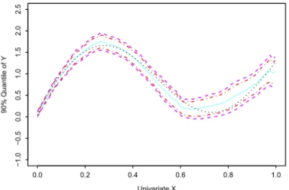
. Based on this normality property, all the assumptions can be seen to be satisfied.

(8)

Fig. 1. The real 0.9 quantile curve (black dotted line), 0.9 quantile estimate (cyan solid line) with corresponding 95% uniform confidence band from asymptotic theory (magenta dashed lines) and confidence band from bootstrapping (red dashed–dot lines). (For interpretation of the references to color in this figure legend, the reader is referred to the web version of this article.)

(2) Compute the local quantile smootherlh

(

x

)

ofY1

, . . . ,

Yn with bandwidthhand obtain residuals

ε

ˆ

i

=

Yi

−

lh

(

Xi

),

i

=

1

, . . . ,

n.

If we choosep

=

0

.

9, thenΦ−1

(

_p

)

=

₁

.

₂₈₁₆

,

_l

(

_x

)

=

_sin

(

_x

)

+

₁

.

₂₈₁₆

√

_x_{. Set}_h

=

₀

.

_05. (3) Compute the conditional edf:

ˆ

F

(

t|x

)

=

n



i=1 Kh

(

x

−

Xi

)

1

{ˆ

ε

i6t} n



i=1 Kh

(

x

−

Xi

)

.

The choice of kernel functions plays a minor role here. Section 3.4.3 and Table 3.3 of Härdle et al. [21] discuss the efficiencies of different kernels. The Epanechnikov kernel would be the optimal one; however, the differences among various kernels are small. Thus, we just use the Gaussian kernel to assure numerical stability. This is also convenient because the optimal bandwidth suggested by Yu and Jones [36] is also calculated based on the Gaussian kernel. (4) For eachi

=

1

, . . . ,

n, generate random variables

ε

_i∗_,_b

∼ ˆ

F

(

t

|

x

),

b

=

1

, . . . ,

Band construct the bootstrap sample

Y∗

i,b

,

i

=

1

, . . . ,

n

,

b

=

1

, . . . ,

Bas follows:

Y_i∗_,_b

=

lg

(

Xi

)

+

ε

i∗,b

,

withg

=

0

.

2.

(5) For each bootstrap sample

{

(

Xi

,

Yi∗,b

)

}

ni=1, computel ∗

hand the random variable

db def

=

sup x∈J∗



ˆ

f

{l

∗_h

(

x

)

|x}



ˆ

fX

(

x

)

|l

∗h

(

x

)

−

lg

(

x

)

|



,

(24)

where

ˆ

f

{l

(

x

)

|x}

,

f

ˆ

X

(

x

)

{l

(

x

)

|x}

,

fX

(

x

)

with use off

(

y|x

)

=

f

(

x

,

y

)/

fX

(

x

)

. (6) Calculate the

(

1

−

α)

quantiled∗_αofd1

, . . . ,

dB.

(7) Construct the bootstrap uniform confidence band centered aroundlh

(

x

)

, i.e.lh

(

x

)

±



ˆ

f

{l

h

(

x

)

|x}



ˆ

fX

(

x

)



−1 d∗ α.

Fig. 1shows the theoretical 0.9 quantile curve, 0.9 quantile estimate with corresponding 95% uniform confidence band from the asymptotic theory and the confidence band from the bootstrap. The real 0.9 quantile curve is marked as the black dotted line. We then compute the classic local quantile estimatelh

(

x

)

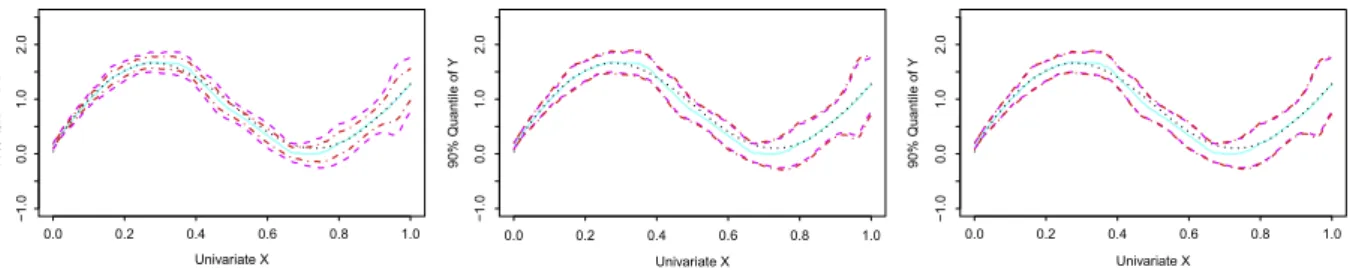
(cyan solid) with its corresponding 95% uniform confidence band (magenta dashed) based on asymptotic theory according to Härdle and Song [22]. The 95% confidence band from the bootstrap is displayed as red dashed–dot lines. At first sight, the quantile smoother, together with two corresponding bands, all capture the heteroscedastic structure quite well, and the width of the bootstrap confidence band is similar to the one based on asymptotic theory in [22].Fig. 2presents the bootstrap confidence bands constructed using different oversmoothing bandwidths w.r.t. the same (but different from the one used forFig. 1) randomly generated data set, namely, 1/2, 1 and 2 times (from left to right) of the oversmoothing bandwidthg

=

n4/45_h_{used before. As we can see,} when we deviate fromg

=

n4/45h, the bootstrap confidence bands get wider.

We now extendxto the multivariate case and use a different quantile function to verify our method. Choosex

=

(

u

, v)

⊤

∈

Rd

, v

∈

R, and generate the data

{

(

Ui

,

Vi

,

Yi

)

}

ni=1

,

n

=

1000 with

y

=

2u

+

v

2

+

ε

−

1

.

2816

,

(25)

where uand

v

are uniformly distributed random variables in

[

0

,

2

]

and

[

0

,

1

]

respectively.

ε

has a standard normal distribution. The theoretical 0.9-quantile curve is

˜

l

(

x

)

=

2u

+

v

2. Since the choice ofanis uncertain here, we test different

(9)

Fig. 2. The real 0.9 quantile curve (black dotted line), 0.9 quantile estimate (cyan solid line) with corresponding 95% uniform confidence band from asymptotic theory (magenta dashed lines) and confidence band from bootstrapping (red dashed–dot lines). The left, middle and right plots correspond to the oversmoothing bandwidth set asn4/45_h_/₂_,_n4/45_h_{and 2}_n4/45_h_{respectively. (For interpretation of the references to color in this figure legend, the reader}

is referred to the web version of this article.)

Table 1

SSE of_βˆ_{with respect to}_a_n_{for different numbers of observations.} an n=1000 n=8000 n=261148 n1/3_/₈ ₃_.₆_×₁₀−3 n1/3_/₄ ₅_.₄_×₁₀−1 ₄_.₀_×₁₀−2 ₃_.₃_×₁₀−3 n1/3_/₂ ₆_.₁_×₁₀−1 ₃_.₅_×₁₀−2 ₃_.₂_×₁₀−3 n1/3 ₆_.₂_×₁₀−1 ₃_.₆_×₁₀−2 ₃_.₁_×₁₀−3 n1/3_·₂ ₈_.₀_×₁₀−1 ₃_.₉_×₁₀−2 ₂_.₉_×₁₀−3 n1/3_·₄ ₄_.₉_×₁₀−1 ₃_.₆_×₁₀−2 ₂_.₈_×₁₀−3 n1/3_·₈ ₃_.₄_×₁₀−3

choices ofanfor differentnby simulation. To this end, we modify the theoretical model as follows:

y

=

2u

+

v

2

+

ε

−

Φ−1

(

p

)

such that the real

β

is always equal to 2 no matter ifpis 0.01 or 0.99. The result is displayed inFig. 3forn

=

1000

,

n

=

8000

,

n

=

261148 (number of observations for the data set used in the following application part including both uncensored and censored observations). Different lines correspond to differentan, i.e.n1/3

/

8

,

n1/3

/

4

,

n1/3

/

2

,

n1/3

,

n1/3

·

2

,

n1/3

·

_{4 and}_n1/3

·

_{8. At first, it seems that the choice of}_a

ndoes not matter too much. To further investigate this, we calculate the SSE (



99

1

{ ˆ

β(

i

/

100

)

−

β

}

) where

β(

ˆ

i

/

100

)

denotes the estimate corresponding to thei

/

100 quantile. The results are displayed inTable 1. Obviouslyanhas much less effect thannon SSE. Considering the computational cost, which increases withan, and the estimation performance, empirically we suggestan

=

n1/3. Certainly this issue is far from settled and needs further investigation.

Thus for the specific model(25), we havean

=

10

,

β

ˆ

=

1

.

997

,

h

=

0

.

2 andg

=

0

.

7. InFig. 4the theoretical 0.9 quantile curve with respect to

v

, and the 0.9 quantile estimate with corresponding uniform confidence band are displayed. The real 0.9 quantile curve is marked as the black dotted line. We then compute the quantile smootherlh

(

x

)

(magenta solid). The 95% bootstrap uniform confidence band is displayed as red dashed lines and covers the true quantile curve quite well.

5. A labor market application

Our intuition of the effect of education on income is summarized by Day and Newburger’s basic claim [7]: ‘‘At most ages, more education equates with higher earnings, and the payoff is most notable at the highest educational levels’’, which is actually from the point of view of mean regression. However, whether this difference is significant or not is still questionable, especially for different ends of the (conditional) income distribution. To this end, a careful investigation of quantile regression is necessary. Since different education levels may reflect different productivity, which is unobservable and may also results from different ages, abilities etc., to study the labor market differential effect with respect to different education levels, a semiparametric partial linear quantile model is preferred, which can retain the flexibility of the nonparametric models for the age and other unobservable factors and ease the interpretation of the education factor.

We use the administrative data from the German National Pension Office (Deutsche Rentenversicherung Bund) for the following group: West German part, males, born between 1939 and 1942 who began receiving a pension in 2004 or 2005 (when they were 62–66 years old) with at least 30 yearly uncensored observations. Since different people entered into the pension system and stopped receiving job earnings at different ages, we only consider those earnings recorded by the pension system when they were between 25 and 59 years old. For example, we consider person A’s yearly earnings when he was 25–59 (entering into the pension system at 25), person B’s when he was 27–59 (entering into the pension system at 27), and person C’s when he was 30–59 (entering into the pension system at 30). In total,n

=

128429 observations are available. We have the following three education categories: ‘‘low education’’, ‘‘apprenticeship’’ and ‘‘university’’ for the variableu(we assign them the numerical values 1, 2 and 3 respectively); the variable

v

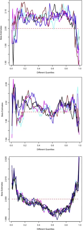
is the age of the employee. ‘‘Low education’’ means without post-secondary education in Germany. ‘‘Apprenticeship’’ means part of Germany’s dual education

(10)

Fig. 3. _βˆ_{with respect to different quantiles for different numbers of observations, i.e.}_n=1000 (top),n=8000 (middle),n=261 148 (bottom). Different lines in the same plot correspond to differentan, i.e.n1/3/8,n1/3/4,n1/3/2,n1/3,n1/3·2,n1/3·4 andn1/3·8.

system. Depending on the profession, a person may work for three to four days a week in the company and then spend one or two days at a vocational school (Berufsschule). ‘‘University’’ in Germany also includes technical colleges (applied universities). Since the level and structure of wages differ substantially between East and West Germany, we concentrate on West Germany only here (which we usually refer to simply as Germany). Our data have several advantages over the most often used German Socio-Economics Panel (GSOEP) data for analyzing wages in Germany. Firstly, they are available for a much longer period, as opposed to from 1984 only for the GSOEP data. Secondly, and more importantly, they have a much larger sample size. Thirdly, wages are likely to be measured much more precisely. Fourthly, we observe a complete earnings

(11)

Fig. 4. Nonparametric part smoothing, real 0.9 quantile curve (black dotted line) with respect tov,0.9 quantile smoother (magenta solid line) with corresponding 95% bootstrap uniform confidence band (red dashed lines). (For interpretation of the references to color in this figure legend, the reader is referred to the web version of this article.)

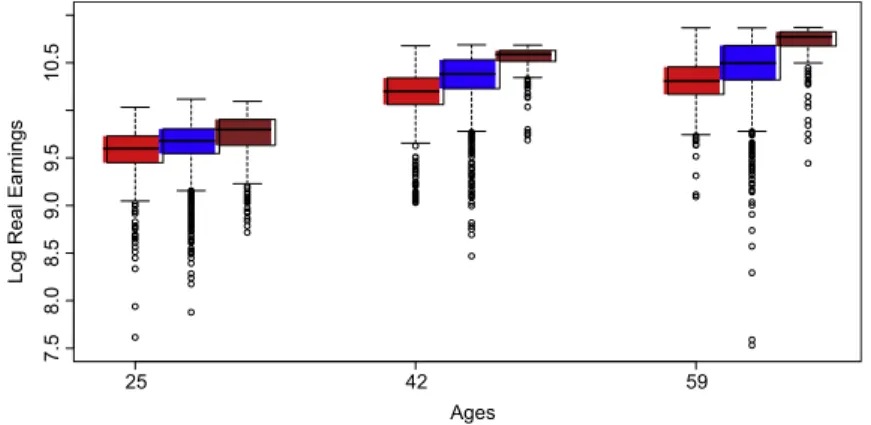
Fig. 5. Boxplots for ‘‘low education’’ (red), ‘‘apprenticeship’’ (blue) and ‘‘university’’ (brown) groups corresponding to different ages. (For interpretation of the references to color in this figure legend, the reader is referred to the web version of this article.)

Fig. 6. _βˆ_{corresponding to different quantiles with 6, 13, 25 partitions.}

history from the individual’s first job until his retirement, therefore this is a true panel, not a pseudo-panel. There are also several drawbacks. For example, some very wealthy individuals are not registered in the German pension system, e.g. if their monthly income is more than some threshold (which may vary for different years due to the inflation effect), the individual has the right not to be included in the public pension system, and thus is not recorded. Besides this, it is also right-censored at the highest level of earnings that is subject to social security contributions, so the censored observations in the data are only for those who actually decided to stay within the public system. Because of the combination of truncation and censoring, this paper focuses on the uncensored data only, and we should not draw inferences from the very high quantile, i.e. we only consider the 0.80 quantiles here. Recently, similar data were also used to investigate the German wage structure as in [9].

(12)

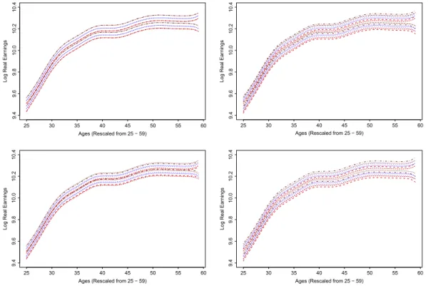
Fig. 7. 95% bootstrap (thick) and asymptotic (thin) uniform confidence bands for 0.20-quantile smoothers w.r.t. 3 different education levels. The ‘‘low education’’, ‘‘apprenticeship’’ and ‘‘university’’ levels are marked as red dashed, blue dotted and brown dashed–dot lines respectively. (For interpretation of the references to color in this figure legend, the reader is referred to the web version of this article.)

Fig. 8. 95% bootstrap (thick) and asymptotic (thin) uniform confidence bands for 0.20-quantile smoothers w.r.t. 3 different education levels with the oversmoothing bandwidth set asg/2,g/4,2gand 4g(from left to right, up to down) respectively. The ‘‘low education’’, ‘‘apprenticeship’’ and ‘‘university’’ levels are marked as red dashed, blue dotted and brown dashed–dot lines respectively. (For interpretation of the references to color in this figure legend, the reader is referred to the web version of this article.)

Following from Becker’s [1] human capital model, a log transformation is performed first on the hourly real wages (unit: EUR, at year 2000 prices).Fig. 5displays the boxplots for the ‘‘low education’’, ‘‘apprenticeship’’ and ‘‘university’’ groups corresponding to different ages. In the data all ages (25–59) are reported as integers and are categorized in one-year groups. We rescaled them to the interval

[

0

,

1

]

by dividing by 40, with corresponding bandwidthshof 0.041, 0.039, 0.041 for the 0.20, 0.50, 0.80 nonparametric quantile smoothers respectively. Correspondingly, as discussed before, we choose g

=

n4/45h, thus 0.12, 0.11, 0.12 for the corresponding oversmoothers respectively. To detect whether a differential effect for different education levels exists, we compare the corresponding uniform confidence bands, i.e. differences indicate that the differential effect may exist for different education levels in the German labor market for that specific labor group.

Following an application of the partial linear model in Section3,Fig. 6displays

β

ˆ

with respect to different quantiles for 6, 13, and 25 partitions, respectively. At first, the

β

ˆ

_{curve is quite surprising, since it is not, as in mean regression, a positive} constant, but rather varies a lot, e.g.

β(

ˆ

₀

.

₂₀

)

=

0

.

026

,

β(

ˆ

₀

.

₅₀

)

=

0

.

057 and

β(

ˆ

₀

.

₈₀

)

=

0

.

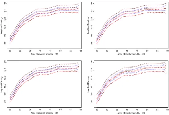
061. Furthermore, it is robust to different numbers of partitions. It seems that the differences between the ‘‘low education’’ and ‘‘university’’ groups are different for different tails of the wage distribution. To judge whether these differences are significant, we use the uniform

(13)

Fig. 10. 95% bootstrap (thick) and asymptotic (thin) uniform confidence bands for 0.50-quantile smoothers w.r.t. 3 different education levels with the oversmoothing bandwidth set asg/2,g/4,2gand 4g(from left to right, up to down) respectively. The ‘‘low education’’, ‘‘apprenticeship’’ and ‘‘university’’ levels are marked as red dashed, blue dotted and brown dashed–dot lines respectively. (For interpretation of the references to color in this figure legend, the reader is referred to the web version of this article.)

confidence band techniques discussed in Section2which are displayed inFigs. 7–11corresponding to the 0.20, 0.50 and 0.80 quantiles respectively.

The 95% uniform confidence bands from bootstrapping for the ‘‘low education’’ group are marked as red dashed lines, while the ones for ‘‘apprenticeship’’ and ‘‘university’’ are displayed as blue dotted and brown dashed–dot lines, respectively. The corresponding asymptotic bands studied in [22] are also added for reference (thin lines with the same style and color), which overlap with the bootstrap bands for large samples as here. For the 0.20 quantile inFig. 7, the bands for ‘‘university’’, ‘‘apprenticeship’’ and ‘‘low education’’ do not differ significantly from one another although they become progressively lower, which indicates that high education does not equate to higher earnings significantly for the lower tails of wages, while increasing age seems to be the main driving force. For the 0.50 quantile inFig. 9, the bands for ‘‘university’’ and ‘‘low education’’ differ significantly from one another although not from that for ‘‘apprenticeship’’. However, for the 0.80 quantiles inFig. 11, all the bands differ significantly (except on the right boundary because of the nonparametric method’s boundary effect) resulting from the relatively large

β(

ˆ

0

.

80

)

=

0

.

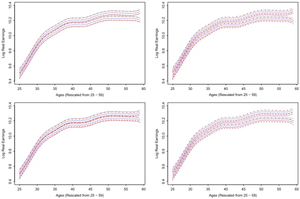
061, which indicates that high education is significantly associated with higher earnings for the upper tails of wages.

(14)

Fig. 12. 95% bootstrap (thick) and asymptotic (thin) uniform confidence bands for 0.80-quantile smoothers w.r.t. 3 different education levels with the oversmoothing bandwidth set asg/2,g/4,2gand 4g(from left to right, up to down) respectively. The corresponding line styles and colors are the same as inFig. 7. (For interpretation of the references to color in this figure legend, the reader is referred to the web version of this article.)

Coupled withFigs. 7,9and11,Figs. 8,10and12present the corresponding bootstrap confidence bands constructed using different oversmoothing bandwidths, namely, half, quarter, twice and quadruple (from left to right, up to down) of the oversmoothing bandwidthg

=

n4/45_h_{used before. The corresponding asymptotic bands are also added for reference} (thin lines with the same style and color). As we can see, in practice, for the typically large labor economic data set, the bootstrap confidence bands are quite robust to the choice of the oversmoothing bandwidth.

If we investigate the explanations for the differences in different tails of the income distribution, maybe the most prominent reason is the rapid development of technology, which has been extensively studied. The point is that technology does not simply increase the demand for upper-end labor relative to that of lower-end labor, but instead asymmetrically affects the bottom and the top of the wage distribution, resulting in its strong asymmetry.

6. Conclusions

In this paper we construct confidence bands for nonparametric quantile estimates of regression functions. The method is based on bootstrapping, where resampling is done from a suitably estimated empirical distribution function (edf) for residuals. It is proven that the bootstrap approximation provides an improvement over the confidence bands constructed

(15)

via the asymptotic Gumbel distribution. We also propose a partial linear model to handle the case of multidimensional and discrete regressor variables. An economic application considering the labor market differential effect with respect to various education levels is studied. The conclusions from the point of view of quantile regression are consistent with those of the (grouped) mean regression, but in a more careful way in the sense that we provide formal statistical tools to judge these uniformly. The partial linear quantile regression techniques, together with confidence bands, developed in this paper display very interesting findings compared with classic (mean) methods and will bring in more contributions to the differential analysis of the labor market.

Appendix

Proof of Theorem 2.1. We start by proving Eq.(8). Write firstF

ˆ

−1

(

_U

i

|X

i

)

=

F−1

(

Ui

|X

i

)

+

∆i. Fix anyisuch that

|F

−1

(

Ui

|X

i

)

−

F−1

(

_p

)

| ≤

_S

n

δ

n, which, by Eq.(1), implies that

|U

i

−

p|

<

Sn

δ

n.Lemma 2.1gives max

i

| ˆ

F

(

S_n2

δ

n

|X

i

)

−

F

(

Sn2

δ

n

|X

i

)

| =

Op

(

Sn

δ

n

).

(26) Together withF

(

±S

_n2

δ

n

|X

i

)

=

p

±

O

(

Sn2

δ

n

)

, again by Eq.(1), we haveF

ˆ

(

±S

2n

δ

n

|X

i

)

=

p

±

Op

(

Sn2

δ

n

)

and thus

ˆ

F

(

−S

_n2

δ

n

|X

i

)

=

p

−

Op

(

Sn2

δ

n

)

6 p

−

Sn

δ

n

<

Ui

<

p

+

Sn

δ

n

<

p

+

Op

(

Sn2

δ

n

)

= ˆ

F

(

Sn2

δ

n

|X

i

).

SinceF

ˆ

(

·|X

i

)

is monotone non-decreasing,

| ˆ

F−1

(

Ui

|X

i

)

| ≤

Sn2

δ

n, which means, bySn2

=

Sn,

| ˆ

F−1

(

Ui

|X

i

)

| ≤

Sn

δ

n

.

(27)

Apply nowLemma 2.1again to Eq.(27), and obtain Sn

δ

n

≥ | ˆ

F{ ˆF−1

(

Ui

|X

i

)

|X

i

} −

F{ ˆF−1

(

Ui

|X

i

)

|X

i

}|

= |U

i

−

F

{F

−1

(

Ui

|X

i

)

+

∆i

|X

i

}|

= |F{F

−1

(

Ui

|X

i

)

|X

i

} −

F{F−1

(

Ui

|X

i

)

+

∆i

|X

i

}|

≥

f₀

(

X_i

)

|

∆_i

|

.

(28)

Hence

|

∆_i

|

<

S_n

δ

_n, and we summarize it as max i:|F−1₍_U i|Xi)−F−1(p)|<Snδn

|

F−1

(

Ui

|

Xi

)

−



F −1

(

Ui

|

Xi

)

| =

Op

{

Sn

δ

n

}

.

To show Eq.(12), define

Z1j def

=

Y_j∗

−

lg

(

Xj

)

+

lg

(

Xj

)

−

lg

(

Xi

),

Z2j def

=

Y_j#

−

l

(

Xj

)

+

l

(

Xj

)

−

l

(

Xi

).

Thusqhi

[{

(

Yj∗

−l

g

(

Xj

)

+l

g

(

Xj

)

−l

g

(

Xi

))

}

nj=1

]

andqhi

[{Y

j#

−l

(

Xj

)

+l

(

Xj

)

−l

(

Xi

)

}

nj=1

]

can be seen aslh

(

Xi

)

for data sets

{

(

Xi

,

Z1i

)

}

ni=1 and

{

(

Xi

,

Z2i

)

}

ni=1respectively. Similarly to Härdle and Song [22], they can be treated as zeros (w.r.t.

θ, θ

∈

IwhereIis a possibly infinite, or possibly degenerate, interval in_R) of the functions



G_n

(θ,

X_i

)

def

=

n−1 n



j=1 Kh

(

Xi

−

Xj

)ψ(

Z1j

−

θ),

(29)



Gn

(θ,

Xi

)

def

=

n−1 n



j=1 Kh

(

Xi

−

Xj

)ψ(

Z2j

−

θ).

(30)

From(8)and(9), we have max i



[{Y

∗ j

−

lg

(

Xj

)

+

lg

(

Xj

)

−

lg

(

Xi

)

}

nj=1

] − [{Y

# j

−

l

(

Xj

)

+

l

(

Xj

)

−

l

(

Xi

)

}

nj=1

]



=

Op

{S

n

δ

n

} +

Op

(δ

n

)

=

Op

(δ

n

).

(31) Thus sup θ∈I max i

|



G_n

(θ,

X_i

)

−



G_n

(θ,

X_i

)

| ≤

O_p

(δ

_n

)

max



n −1



Kh



=

Op

(δ

n

).

(16)

To show the difference of the two quantile smoothers, we shall reduce the strong convergence ofqhi

[{Y

j∗

−

lg

(

Xj

)

+

lg

(

Xj

)

−

lg

(

Xi

)

}

nj=1

] −

qhi

[{Y

j#

−

l

(

Xj

)

+

l

(

Xj

)

−

l

(

Xi

)

}

nj=1

]

, for anyi, to an application of the strong convergence of



G

(θ,

X_i

)

to



G_n

(θ,

X_i

)

,

uniformly in

θ

, for anyi. Under assumptions (A7) and (A8), in a similar spirit to Härdle and Song [22], we get max

i

|l

∗

h

(

Xi

)

−

lg

(

Xi

)

−

l#h

(

Xi

)

−

l

(

Xi

)

| =

Op

(δ

n

).

To show the supremum of the bootstrap approximation error, without loss of generality, based on assumption (A1), we reorder the original observations

{X

i

,

Yi

}

ni=1, such thatX16X26

, . . . ,

6Xn. First decompose:

sup x∈J∗

|l

∗_h

(

x

)

−

lg

(

x

)

−

l#h

(

x

)

−

l

(

x

)

| =

max i

|l

∗ h

(

Xi

)

−

lg

(

Xi

)

−

l#h

(

Xi

)

+

l

(

Xi

)

|

+

max i x∈[Xsupi,Xi+1]

|l

∗_h

(

x

)

−

lg

(

x

)

−

l#h

(

x

)

+

l

(

x

)

|

.

(32) From assumption (A1) we knowl′

(

·

)

≤

λ

₁and maxi

(

Xi+1

−

Xi

)

=

Op

(

Sn

/

n

)

. By the mean value theorem, we conclude that the second term of(32)is of a lower order than the first term. Together with Eq.(12)we have

sup x∈J∗

|l

∗_h

(

x

)

−

lg

(

x

)

−

lh#

(

x

)

−

l

(

x

)

| =

O

{

max_i

|l

∗

h

(

Xi

)

−

lg

(

Xi

)

−

l#h

(

Xi

)

−

l

(

Xi

)

|} =

Op

(δ

n

),

which means that the supremum of the approximation error over allxis of the same order of the maximum over the discrete observedXi.

Proof of Theorem 2.2.The proof of(16)uses methods related to those in the proof of Theorem 3 of Härdle and Marron [20], so only the main steps are explicitly given. The first step is a bias-variance decomposition,

E





ˆ

bh,g

(

x

)

−

bh

(

x

)



2

|X

1

, . . . ,

Xn



=

Vn

+

Bn2

,

(33) where Vn

=

Var



ˆ

bh,g

(

x

)

|X