Sentiment Analysis and Opinion Mining on Twitter with GMO Keyword

(1)

SENTIMENT ANALYSIS AND OPINION MINING ON TWITTER WITH GMO KEYWORD

A Paper

Submitted to the Graduate Faculty of the

North Dakota State University of Agriculture and Applied Science

By Hanzhe Li

In Partial Fulfillment of the Requirements for the Degree of

MASTER OF SCIENCE

Major Department: Computer Science

May 2016

(2)

North Dakota State University

Graduate School

Title

SENTIMENT ANALYSIS AND OPINION MINING ON

TWITTER WITH GMO KEYWORD By Hanzhe Li

The Supervisory Committee certifies that this disquisition complies with North Dakota

State University’s regulations and meets the accepted standards for the degree of

_{MASTER OF SCIENCE} SUPERVISORY COMMITTEE: Dr. Kendall Nygard Chair Dr. Juan (Jen) Li Dr. Yarong Yang Approved: 06/17/2016 Dr. Brian Slator

(3)

ABSTRACT

Twitter are a new source of information for data mining techniques. Messages posted through Twitter provide a major information source to gauge public sentiment on topics ranging from politics to fashion trends. The purpose of this paper is to analyze the Twitter tweets to discern the opinions of users regarding Genetically Modified Organisms (GMOs).

We examine the effectiveness of several classifiers, Multinomial Naïve Bayes, Bernoulli Naïve Bayes, Logistic Regression and Linear Support Vector Classifier (SVC) in identifying a positive, negative or neutral category on a tweet corpus. Additionally, we use three datasets in this experiment to examine which dataset has the best score. Comparing the classifiers, we discovered that GMO_NDSU has the highest score in each classifier of my experiment among three datasets, and Linear SVC had the highest consistent accuracy by using bigrams as feature extraction and Term Frequency, Chi Square as feature selection.

(4)

ACKNOWLEDGEMENTS

I would like to express my sincerest gratitude to the following individuals:

Dr.Kendall Nygard, my major advisor, thank you for your help, instruction, and advice during the courses of my graduate education and the preparation for this paper. Thank you for your help and encouragement, and providing the advice which is used in this paper. I appreciate that you gave me an assistantship. Thank you for your trust.

Dr. Juan Li and Dr. Yarong Yang, thank you for serving as my graduate committee and giving me encouragement and insightful comments.

Matthew Warner, thank you for your guidance on my writing skill. It is hard to review my paper, especially after I moved, but you have given me the best support under the

circumstances. Thank you for your suggestions.

Xiaoxue Gu, my wife, thank you for you being in my life, giving me infinite love, understanding, support, and encouragement. You have been there for me and I know you will always be there for me.

(5)

DEDICATION

This paper is dedicated to my parents. For their endless love, support and encouragement.

(6)

LIST OF TABLES

Table Page

1. Classification of Words and Phrases Relative to GMO ... 5

2. Format of Single Tweet Related to GMO ... 8

3. Tokenized Text after Remove Irrelevant Information from Original Tweets ... 9

4. List of Stopwords of NLTK ... 10

5. Example of Text after Removing Symbols ... 11

6. Example of Most Informative Features for Unigram ... 13

7. Example of Most Informative Features for Bigrams ... 14

8. Result of Three Datasets Analyzed by Four Classifiers, TF and Unigram ... 23

9. Result of Three Datasets Analyzed by Four Classifiers, TF and Bigrams ... 24

10.Result of Three Datasets Analyzed by TF-IDF and Unigram Includes Stopwords ... 26

11.Result of Three Datasets Analyzed by TF-IDF and Unigram Excludes Stopwords ... 28

12.Result of Three Datasets Analyzed by Four Classifiers, TF-IDF and Bigrams ... 30

13.Result of Three Datasets Analyzed by Chi Square with Bigrams ... 31

14.Result of 2 Classes and 3 Classes Analyzed by Four Classifiers with TF ... 33

15.Result of 2 Classes and 3-Classes Analyzed by Four Classifiers with TF-IDF ... 33

16.Results for Unigram and Bigrams Analyzed by TF ... 34

17.Results for Unigram and Bigrams Analyzed by TF-IDF ... 34

18.Value of Best Feature Selection Analyzed by Four Classifiers ... 35

19.Value of N-Fold and Leave-One-Out Cross Validation ... 37

(9)

LIST OF FIGURES

Figure Page

1. Overall View of Classification ... 12

2. Basic Feature Selection Algorithm ... 16

3. Result of Three Datasets Analyzed by Four Classifiers, TF and Unigram ... 23

4. Result of Three Datasets Analyzed by Four Classifiers, TF and Bigrams ... 25

5. Result of Three Datasets Analyzed by TF-IDF and Unigram Includes Stopwords ... 27

6. Result of Three Datasets Analyzed TF-IDF and Unigram Excludes Stopwords ... 28

7. Result of Three Datasets Analyzed by TF-IDF and Bigrams ... 30

8. Result of Three Dataset Analyzed by Chi Square with Bigrams ... 32

9. Value of Best Feature Selection Analyzed by Four Classifiers ... 36

10.Geographic Data Related to GMO Shown in the World Map ... 44

(10)

1. INTRODUCTION

Over the course of one day, Twitter users will post and re-post a tremendous volume of messages. On some occasions, over half of a billion Tweets are sent per day, which approximates to a rate of 5787 Tweets/second. This volume of messages has produced a large corpus of

messages that represent the opinions and insights of users. Recently, data-miners and other researchers have dedicated more attention to analyzing the meaning of Twitter posts in order to more accurately understand public sentiment.

Sentiment can be challenging to analyze even in a large corpus like Twitter posts.

However, topics deemed controversial provide an excellent entry point to analyzing sentiment. A controversial topic divides people into groups depending on their opinions. Following this

reasoning, we selected Genetically Modified Organisms (GMOs) as our topic to perform sentiment analysis. GMOs is a controversial topic. As a consequence of the controversy, we anticipate a particular pattern to user postings. Some users post that they refuse to eat any food products containing genetically modified organisms. Other users state that they perceive no problems consuming food products containing GMOs. A third possibility is that there are many users who don’t have any opinion on food products containing GMOs. Based on this reasoning, GMOs is an excellent topic to analyze the sentiment of Twitter postings for identifying patterns and groupings.

In this paper, we examine the opinions and sentiments of Twitter users concerning the GMOs and non-GMOs debate. We want to identity, based on the Twitter corpus, which aspect of GMOs garners the greatest concern from the users. To analyze the corpus, we apply four

machine learning techniques that are commonly used for classification, and test the accuracy on the Twitter corpus.

(11)

2. RELATED WORK

With the popularity of Tweets and social online media creating a steadily increasing collection of data, opinion mining and sentiment analysis has become a field of interest for increased research. The techniques to collect data include ways to pre-process sentences, like tokenization, stop words removal and stemming, and feature selection. Pak [1] collect two types of emoticons for collected corpora from Tweets to form a training dataset for recognizing positive and negative sentiments based on happy and sad emotions. The classifier was implemented by the Multinomial Naïve Bayes that uses N-gram which meansa contiguous sequence of n items from a given sequence of text or speech and POS-tags which means the process of marking up a word in a text (corpus) as corresponding to a particular part of speech to extract features. An N-gram of size 1 is referred to as a "unigram"; size 2 is a "bigram" (or, less commonly, a "digram"). Additionally, they increased the accuracy of the classification by using Entropy and Salience methods.

Similar to the work of Pak, Zhang [2] describes work with the same training set collection and saves it into MongoDB. The author compared three classifiers, including Naïve Bayes, Maximum Entropy and Support Vector Machine that uses Chi-Squared Information Gain and term frequency–inverse document frequency (TF-IDF) as Feature Filtering. Author got the SVM is the best approach as his research result based on Accuracy, Positive/Negative Precision, Positive/Negative Recall.

Kouloumpis [4] evaluates training data which included a Hashtagged data set, Emoticon data set and iSieve data set with labels derived from hashtags and emoticons is beneficial for training sentiment analysis in Tweets. It is shown that the result of sentiment analysis didn’t achieve satisfaction while using part-of-speech features for features extraction.

(12)

Turney [5] classifies reviews as recommended or not recommended according to an unsupervised learning algorithm. The algorithm in this Sentiment analysis which calculated the difference of mutual information between good associations (e.g., “excellent”) and bad

associations (e.g., “poor”).The sentiment lexicon is the most utilized resource for most sentiment analysis algorithms [6].

In order to clean data before analyzing, Bifet and Frank [7] remove the character @, Hashtags, RT (retweet), only analysis textual sentiment in Tweets.

The message in Twitter is essentially used for convey information to the person who has the same idea or opinion rather than arguing some issue on the twitter post-wall [3].

Using large number of features at 10000 and 15000 can help to improve accuracy, precision and recall a lot rather using very few features [9].

Authors perform test on three datasets, confirmed that part of Speech-Based Selection are important for polarity classification. Meanwhile, using stemming in text pre-processing doesn’t give a better accuracy [19].

(13)

3. CORPUS COLLECTION

Before training a sentiment analyzer and obtaining data, we needed to collect our own dataset to compare with several existing datasets which are used for sentiment analysis on Twitter. We perform tests on three datasets.

First comes from Pang and Lee [8] and includes 5331 positive and 5331 negative movie review as we called “Movie_Review” dataset from IMDB, meanwhile it is a general sentiment dataset for normal analysis. However, we don’t know the result and accuracy if we are going to use “Movie_Review” dataset as analyzing the specific topic like GMO debate. We will try this dataset and have a comparison with other datasets.

Second dataset called “GMO_Hedge” which is the data for studying hedging and framing in GMO debates and in professional vs. pop-science discourse by Choi, Tan and Lee [10]. It is the first dataset which is related to the GMOs that I found online. Anti-GMO contains 10314 instances and pro-GMO contains 8963 instances which are processed we can use it directly. GMOs hedge provides corpora that distinguishes popular-science text from text written by professional scientists, which means tweets are considered popular-science text is mostly from internet buzz words will make more confused meaning than professional science paper [10]. It is the first time to use GMOs hedge as data on sentiment analysis, we will see the result from this dataset.

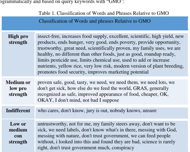
Third dataset is using the words in Table 1 and collecting tweets that contain each word shown in Table 1 which from a survey of GMOs classification and “GMO” as keywords connected Twitter REST API to retrieve Tweets. Firstly, I split the data into three categories (only positive, negative and neutral) to test the accuracy of several classification algorithms. In Table 1, I needed to combine the four categories into two categories. After collecting a large

(14)

corpus into the “strong positive”, “medium positive”, “strong negative”, and “medium negative” categories, I merged “strong positive” and “medium positive” to form “positive”, and “strong negative” and “medium negative” to form “negative”, and remain “Indifferent” as “neutral”. But we did not use the “indifferent” or “neutral” class in the first serval comparisons, since there is no “neutral” category in previous two datasets. Each dataset (pro and con) was collected programmatically and based on query keywords with “GMO”:

Table 1. Classification of Words and Phrases Relative to GMO Classification of Words and phrases Relative to GMO

High pro strength

insect-free, increases food supply, excellent, scientific, high yield, new products, ends hunger, very good, ends poverty, provide opportunity, trustworthy, great need, scientifically proven, my family uses, we are healthy, no different than other foods, just as good, roundup ready, limits pesticide use, limits chemical use, used to add or increase nutrients, yellow rice, very low risk, modern version of plant breeding, promotes food security, improves marketing potential

Medium or low pro strength

proven safe, good, tasty, we need, we need them, we need lots, we don't get sick, how else do we feed the world, GRAS, generally recognized as safe, improved appearance of food, cheaper, OK, OKAY, I don't mind, not bad I suppose

Indifferent who cares, don't know, jury is out, nobody knows, unsure

Low or medium

con strength

untrustworthy, not for me, my family steers away, don't want to be sick, we need labels, don't know what's in there, messing with God, messing with nature, don't trust government, we can feed people without, i looked into this and found they are bad, science is rarely right, don't trust government much, conspiracy

After collecting raw data, our research group members manually classified around 300 Tweets to use in a supervised classification in which randomly tweets were from the dataset where I collected Tweets based on above keywords into three classes, namely positive, negative and neutral. I named this dataset as GMO_NDSU.

(15)

We compared those three datasets with only two classes (positive and negative), pick the one which has the highest accuracy score by using four classifiers.

After the best dataset selected, we also considered including a “neutral” class label, but we were uncertain how that class would influence sentiment accuracy. Based on Andy’s approach [9], including a “neutral” class significantly decreased sentiment accuracy. However, Koppel and Schler [20] argued that “Neutral” class/category should not be ignored, the author proved some of classifier can get a better accuracy while add “neutral” as category.

We will also have a comparison among those classifiers, feature extraction approaches, and find out which is the best to suit out experiment.

3.1. Streaming API

Twitter provides developers and scholars two APIs to collect Tweets: Streaming API and Search API. The APIs are very similar. However, one distinction is that the Streaming API allows developers to retrieve Tweets in real-time with an input query. When using Streaming API, a developer first requests a connection to a stream of Tweets from the server, the server will ask keys and access token (like, OAuth) which Twitter Application Management provides them to users. After the server verifies keys and access token (like, OAuth) that are obtained from Twitter Application Management, the developer has access to a streaming connection of Tweets as they occur.

The advantage of Streaming API is the real-time view of user posting. A developer can view postings as they happen which provides insight into trends in during a given time frame. However, Streaming API has a few limitations for the current research. First, even though there are 180,000 Tweets per hour in all over the world, it slowly retrieve the data at a short moment if we only want to filter the Tweets with “GMO” keyword. Additionally, at the free level, the

(16)

streamed Tweets are only a small fraction of the actual Tweet body (gardenhose vs. firehose). Initial testing with the streaming API caused in an uncompleted training dataset as it proved difficult to obtain too much Tweets which is related to GMO keywords.

3.2. Twitter Search API

Search API is part of Twitter’s REST API, it searches recent Tweets published in the past 7-10 days, which is focused on relevance and not completeness. Although, Search API also has some limits, like only query data past 7-10 days, some Tweets and users may be missing from search result since not completeness, but it has a wider range of data and get Tweets with “GMO” keywords much faster than Streaming API. Because of these issues, we decided to go with the Twitter Search API instead.

The Search API allows finer tuning of queries, including filtering based on language, region, and time. There is a rate limit associated with the query, but we handle it in the code. For our purposes, the rate limit has not been an issue. To actually fetch Tweets, we continuously send queries to the Search API, with a small delay to account for the rate limit. The query (shown below) is constructed by stringing separate keywords together with an “OR” in between. Though this is also not a fully complete result, it returns a well filtered set of Tweets that is useful for our sentiment analyzer. The request returns a list of JSON objects that contain the Tweets and their metadata. This includes a variety of information, including username, time, location, RE-Tweets, and more. For our purposes, we mainly focus on the tweet text and geographic data. An example of common tweet characters and formats can be seen in Table 2.

(17)

Table 2. Format of Single Tweet Related to GMO

Original Single Tweet in Twitter

{

"in_reply_to_status_id_str":"600473614786252801", "in_reply_to_status_id":600473614786252801, "created_at":"Tue May 19 02:36:55 +0000 2015", "retweeted":false,

"in_reply_to_screen_name":"BMarieChagollan", "id":600490285144023041,

"text":"@BMarieChagollan cute avi", "place":{

"country_code":"US", "country":"United States", "full_name":"Orange, CA", "bounding_box":{ "coordinates":[ ]

"user":{

"profile_background_image_url":"http://abs.twimg.com/images/themes/theme1/bg.png", "description":"obsessed with churros and Anthony",

"created_at":"Wed Dec 25 19:11:34 +0000 2013",

"profile_background_image_url_https":"https://abs.twimg.com/images/themes/theme1/b g.png",

"screen_name":"bigbuttbartolo", "name":"Katie Bartolo",

} }

In this paper, I retrieved the data from “text” tag from Table 2 in each Tweet since I mainly focus on text analysis. Furthermore, I collected coordinates as well to illustrate geographic data on the map and filtered rest of tags in Tweets out.

Same way like Streaming API, Search API require the user have an API key for

authentication. Once authenticated, we were able to easily access the data through Twitter Search API, a Python library that operates as a simple wrapper for the Twitter API.

(18)

4. TWEET TEXT PROCESSING

After collecting my raw dataset, I processed the tweet text before analysis. Each tweet contains much irrelevant content that will affect analysis of sentiment. For example, many Tweets include URLs, tags to other personal information, or symbols that have no meaning for this experiment. To precisely get a tweet’s sentiment, we first need to remove these nuisances from the text of the Tweets.

4.1. Tokenization

This process involves splitting the text by spaces, forming a list of individual words per text. This is also called a bag of words. We will later use each word in the tweet to form feature extraction approach to train our classifier. I use “word_tokenize” method from nltk library to process tokenization.

from nltk import word_tokenize tokens = word_tokenize(raw_data)

Table 3. Tokenized Text after Remove Irrelevant Information from Original Tweets

Number of Tweets

Tokenized Text/Status after remove other irrelevant information from original Tweets

1 ['stupid', 'wife', 'red', 'bow', 'spaw', 'yellow', 'stripper', 'gmo', 'everything', 'letters', 'camila', 'gt', 'minhas', 'ruínas']

2 ['Our', 'Photovoltaic', 'systems', 'guaranteed', '100', 'Organic', 'non', 'GMO', 'Solal', 'free', 'FDA', 'approved', 'http://t.co/NxSE1HYTHj'] 3 ['I', 'happy', 'favorite', 'mayo', 'I', "hadn't", 'bought', 'YEARS',

'Non-GMO', 'I', 'thought', 'I', 'saw', 'http://t.co/9OgQifc32E']

In Table 3 shown that Tweets after processing by tokenization. However, those tokenized text still have some meaningless single words, like “gt”, “mayo” and “I”, we have to remove these words in the next further experiment.

(19)

4.2. Stopwords Removal

Another option is we can remove stopwords from the bag of words. Python’s Natural Language Toolkit (NLTK) library contains a stopword dictionary. To remove the stopwords from each text, we simply check each word in the bag of words against the dictionary. If a word is a stopwords, we filter it out. The list of stopwords contains words that signify no sentiment value, such as articles and prepositions (Table 4).

from nltk.corpus import stopwords stopwords.words('english') Table 4. List of Stopwords of NLTK Stopwords

‘I’, ‘you (singular), thou’, ‘he’, ‘we', 'you (plural)', 'they', 'this', 'that', 'here', 'there', 'who', 'what', 'where', 'when', 'how', 'not', 'all', 'many', 'some’, ‘few', 'other', 'one', 'two', 'three', 'four', 'five', 'big', 'long', 'wide'

NLTK includes a Swadesh wordlist that consists of about 200 common words of several languages. The languages are identified using an ISO 639 two-letter code.

4.3. Removing Twitter Symbols

We also found that there are some features that could affect my experiment’ result, which included “http://t.co/NxSE1HYTHj”, “@” or “#” in the Table 3 so that we have to remove these as well.

Many Tweets contain non-alphabetic symbols such as “@” or “#” as well as active web links. The word immediately following the “@” symbol indicates a username, which we filter out entirely. The username is deemed to add no sentiment value to the text but could prove instrumental in performing network analysis of user activities. Words following “#”, known as the hashtag, are also remove, even if text connected to the hashtag contains information used for categorization. The focus of this experiment is textual analysis, and hashtag is assumed to make

(20)

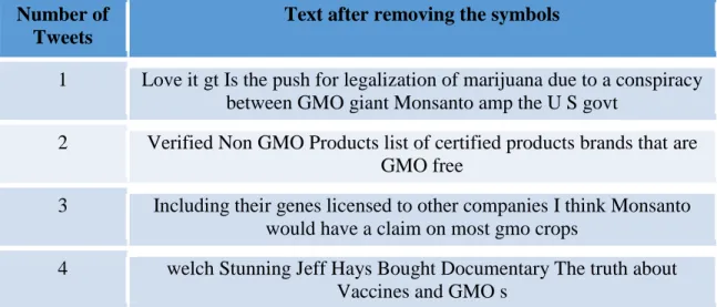
no contribution to the text of an individual message. URLs are filtered out entirely, as they add no sentiment value to the text. To eliminate non-alphabetic symbols, we used a regex that matches for these symbols. Additionally, any non-word symbols in the bag of words are filtered out as well. Examples of Tweets cleaned for non-alphabetic symbols are available in Table 5. tweetRemove = tweet[‘text’]

tweetRemove = ' '.join(re.sub("English(RT)|@[A-Za-z0-9]+)|[^0-9A-Za-z\t])|(\w+:\/\/\S+)"," ",tweetRemove).split())

Table 5. Example of Text after Removing Symbols

Number of Tweets

Text after removing the symbols

1 Love it gt Is the push for legalization of marijuana due to a conspiracy between GMO giant Monsanto amp the U S govt

2 Verified Non GMO Products list of certified products brands that are GMO free

3 Including their genes licensed to other companies I think Monsanto would have a claim on most gmo crops

4 welch Stunning Jeff Hays Bought Documentary The truth about Vaccines and GMO s

Using regular expression to remove symbols in text content, we can get text without symbols.

After these three text pre-process, we are able to analyze Tweets. In the below part, I describe the training of classifiers.

(21)

5. TRAINING THE CLASSIFIERS

Since we have three large datasets, it is important to select the best features when training our datasets in order to reduce the time on the task. For the purpose of training our classifying techniques, we select informative features using several approaches. Once we selected features, we can build and train our classifiers. We will examine four classifiers: Multinomial Naïve Bayes, Bernoulli Naïve Bayes, Logistic Regression and Linear SVC.

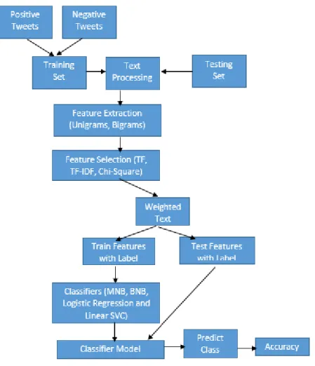
Figure 1. Overall View of Classification

Figure1. Illustrates that the overall process of classification. We will go though it in the next sections.

(22)

5.1. Feature Extraction

In this paper, we introduced unigram and bigrams as feature extraction. We will show the performance for unigram and bigrams respectively and determine which feature extraction will be used in the later research.

5.1.1. Unigram

Unigrams is the simplest approach in N-grams which only obtain one word. For each single word in the text of Tweets, a Unigrams is created for the feature selection to weight text. We examine the classifier to determine which features it found most effective for distinguishing the sentiment’s categories. We used GMO_NDSU dataset and printed first 13 best-feature as shown below:

Table 6. Example of Most Informative Features for Unigram

Most Informative Features Unigramsss Category

risks = True neg : pos = 69.8 : 1.0 negative drugs = True neg : pos = 52.7 : 1.0 negative herbicides = True neg : pos = 48.7 : 1.0 negative bad = True neg : pos = 45.5 : 1.0 negative healthy = True pos : neg = 39.1 : 1.0 positive conspiracy = True neg: pos = 38.7 : 1.0 negative frankenfood = True neg : pos = 32.8 : 1.0 negative sustainable = True pos : neg = 32.5 : 1.0 positive opposed = True neg : pos = 30.3 : 1.0 negative

(23)

Table 6 shows that the categories in the training set that word for "risks" is 69.8 times as negative more often than it classified as positive. However, Unigrams for "sustainable” is 32.5 times in positive more often than they are negative. These ratios are known as likelihood ratios,

and can be useful for comparing different feature-outcome relationships. 5.1.2. Bigrams

Bigrams are features consisting of sets of two adjacent words or pairs of sequence words in a sentence. Unigram sometime cannot capture phrases and multi-word expressions, effectively disregarding any word order dependence. We used GMO_NDSU dataset and printed first 9 best-feature as shown below:

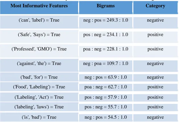
Table 7. Example of Most Informative Features for Bigrams

Most Informative Features Bigrams Category

('can', 'label') = True neg : pos = 249.3 : 1.0 negative ('Safe', 'Says') = True pos : neg = 234.1 : 1.0 positive ('Professed', 'GMO') = True poa : neg = 228.1 : 1.0 positive ('against', 'the') = True neg : poa = 109.7 : 1.0 negative ('bad', 'for') = True neg : pos = 63.9 : 1.0 negative ('Food', 'Labeling') = True poa : neg = 62.7 : 1.0 positive ('Labeling', 'Act') = True pos : neg = 57.9 : 1.0 positive ('labeling', 'laws') = True pos : neg = 55.7 : 1.0 positive ('is', 'bad') = True neg : pos = 54.5 : 1.0 negative

As shown in Table 7, 'Food' and 'Labeling' are two adjacent words defined as positive, while 'is' and 'bad' these two sequence words treat as negative. In previous research, researchers have different opinions on Unigrams and Bigrams. Pang and Lee reported that Unigrams has a

(24)

high accuracy than Bigrams when performing the sentiment classification of movie reviews [8]. In contrast to Pang and Lee, Dave and Lawrence found that Bigrams worked better than

Unigrams for the product-review polarity classification [11]. 5.1.3. Part of Speech Tagging

For each tweet, we have features for counts of the number of the verbs, adverbs, adjectives, nouns, and any other parts of speech. However, POS tags were not useful for

sentiment analysis in the microblogging domain [4]. The accuracy of MaxEnt (equals to Linear Regression/Linear SVC) was slightly increase when compared to Unigrams, the accuracy for Naïve Bayes and SVM are lower than Unigrams result [8].

Since we have a bunch of comparisons in next chapter, we aren’t planning to use part of Speech tags as our feature extraction in this experiment. Unigrams and Bigrams are selected as feature extraction in below experiment.

5.2. Information Gain - Feature Selection

In a large amount of Unigrams or Bigrams, we should select more informative words so that can reduce time consuming for classifiers. Furthermore, it can increase classifier accuracy by eliminating noise features. Based on the performance of the approach with the training set and findings from previous research [22], we performed three measures of information gain, Term-Frequency, TF-IDF (Term Frequency-Inverse Document Frequency) and Chi-Square. The weight of each Unigrams or Bigrams in the dataset is calculated by TF-IDF, Term-Frequency or Chi-Square respectively, so that it become easier to determine the high score words as feature to be used in a further processing.

(25)

Figure 2. Basic Feature Selection Algorithm

The general algorithm for selecting K-best feature shown in Figure 2, we select first K features to train four classifiers.

5.2.1. TF-IDF

TF-IDF calculates [23] score for each word in the dataset described as below:

IDF × TF = IDF -TF t,d t,d t where t t DF N log IDF 

TFt,d is the number of occurrences ofterm t in document d, N is the number of documents in the collection and DFt is the number of documents in the collection that contain term t.

Essentially, TF-IDF avoids assigning high scores to terms that occur too often in the dataset. 5.2.2. Term frequency

Term frequency defines the relative frequency of a term in the document described as below: j j , i / Fd F = TF) Frequency( Term

Fij is total occurrences of the term i in the document j. Fdf is total number of terms occurring in document j.

(26)

5.2.3. Conditional Term frequency

A conditional frequency distribution is a collection of frequency distributions, each one for a different "condition". The condition will often be the category of the text [25]. For example, we will calculate each feature’s conditional term frequency based on “positive” and “negative” category.

5.2.4. Chi-Squared

In statistics, the Chi-Squared test is applied to test the independence of two events, where two events A and B are defined to be independent. It is used to determine whether there is a significant association between the two variables.

Expected frequencies

n n n

E_r_,_c ( _r _c)/

where Er,c is the expected frequency count for level r of Variable A and level c of Variable B, nr is the total number of sample observations at level r of Variable A, nc is the total number of sample observations at level c of Variable B, and n is the total sample size.

Test statistic







  O_r_,_c E_r_,_c 2 E_r_,_c 2 / ) ( 

where Or,c is the observed frequency count at level r of Variable A and level c of Variable B, and Er,c is the expected frequency count at level r of Variable A and level c of Variable B.

(27)

6. CLASSIFICATION

Classification is identifying to which category an object belongs. Some common

applications of classification are spam detection, image recognition, and sentiment analysis. We want to build a classifier with a set of training data and labels. In our case, we want to construct a classifier that is trained on our "positive", "negative" or “neutral" labeled tweet corpus. From this, the classifier will be able to label future Tweets based on the Tweet's attributes or features. In this paper, we examine four common classifiers: Bernoulli Naïve Bayes, Multinomial Naïve Bayes, Logistic Regression and Linear SVC.

6.1. Multinomial Naïve Bayes

With a multinomial event model, samples (feature vectors) represent the frequencies with which certain events have been generated by a multinomial where is the probability that event i occurs (or K such multinomials in the multiclass case).

Multinomial Naive Bayes is a specialized version of Naive Bayes that is designed more for text documents. Whereas simple naive Bayes would model a document as the presence and absence of particular words, multinomial naive bayes explicitly models the word counts and adjusts the underlying calculations to deal with in.

It represents each message as a set if terms m = {t1 ,..., tn}, computing each one of tk as many times it appears in m. In this sense, m can be represented by a vector x = <x1, x2... xn>, where each xk corresponds to the number of occurrences of tk in m. Moreover, each message m of category ci can be interpreted as the result of picking independently | m | terms from T’ with replacement and probability P

 

t_kc_i for each tk. Hence, _

     i c x

P is the multinomial distribution.

 

_

 

         n k k x i k i x c t P m m P c x P k 1 ! |!. | . | |

(28)

Probabilities P

 

t_kc_i are estimated as a Laplacian prior

 

i i k c c t i k N n N c t P   1 , _{, where} i kc N_t _, is the

number of occurrences of term tk in the training messages of category ci, and 



n_ i k Ntkci

N_c _,

i .

6.2. Bernoulli Naïve Bayes

Using Bernoulli Naïve Bayes which a document is represented by a feature vector with binary elements taking value 1 if the corresponding word is present in the document and 0 if the word is not present.

Let T’ = {t1 ,..., tn} the set for terms after term selection. The Bernoulli Naïve Bayes represents each message m as a set of terms by computing the presence or absence of each term. Therefore, m can be represented as a binary vector x= <x1, x2... xn>, where each xk shows whether or not tk will occur in m. The probabilities 

     i c x P are computed by

 



 



 k k x i k x n k i k i P t c Pt c c x P           

_

1 1 1 .

and P

 

t_k c_i and estimated as

 

i i k c c t i k Tr Tr c P    2 1 t , , where i k c t

Tr _, is the number of training

messages of category c_i that contain the term t_kand

i c

Tr is the total number of training messages of category c_i. For more theoretical explanation, consult Losada and Azzopardi [26].

6.3. Logistic Regression

Logistic regression measures the relationship between the categorical dependent variable and one or more independent variables by estimating probabilities using a logistic function, which is the cumulative logistic distribution.

(29)

Mount [14] execute the dataset by using Logistic Regression since the function of Logistic Regression and Maximum Entropy modeling are equivalent. Logistic Regression is a popular algorithm to analyze models for data category, especially for output that is Boolean. Logistic Regression predicts probability (bound to a range of (0, 1)). Probability determined using logistic regression has greater precision compared to probability that is determined by many other classifiers, including Naïve Bayes. We consider features F: = F1, F2...Fn and outcome x which takes binary value (0 or 1). Compared to Naïve Bayes, the features of Logistic

Regression have dependence assumptions which means N-grams features like bigrams can be analyzed by Logistic Regression without worrying about overlapping. The model is represented by the following: )] , ( exp[ )] , ( exp[ ) , | ( , , , , , f c d d c f d c P c i c i i c c i c i i       

In this equation, c is a class (e.g., positive or negative), d is the text of Tweets, and λ is a weight vector which can value the significance of a feature in classification. A higher weight value means that the feature is a highly recommend indicator for the class, and fi,c(c,d) is a binary function that indicates a feature d and a class label c. It is defined as:

      otherwise 0, c and 0 n(f) 1, ) , ( , , , c d c F_i_c

We use the Python package sklearn to perform Logistic Regression classification. Academically, Logistic more efficiently processes bigrams than Naïve Bayes. Though Logistic Regression performs better under these conditions, Naïve Bayes remains a useful approach for other problems [13].

(30)

6.4. Linear SVC

The forth classifier we use in our analysis is the Linear SVC. Linear SVC is another implementation of Support Vector Classification for the case of a linear kernel. Linear SVC can process multi-class classification on a dataset.

In SVM approach, a classifier identifies a dividing line between two separable classes. After analyzing a training dataset, the hyper plane will be formed that functions to separate classified features into the two groups. Additionally, the hyper plane maximizes the distance between the nearest data points of each group. The margin between the hyper plan and the nearest data points is called support vector. In essence, SVM becomes solving an optimization problem:

𝑠. 𝑡. 𝑐i(𝛼 ∙ 𝑓i + 𝑏) ≥ 1 ∀1, … , 𝑛

Here, α is parameter vector that maximizes the distance between the hyper plane and each training point, ci is the class label, ｛1, -1｝for positive and negative, that corresponds to the training feature vector fi.

α α 2 1  Minimize

(31)

7. EXPERIMENT EVALUATION

In this experiment, I used scikit-learn which is a Python open source machine learning library feature some kinds of classifications, regression and clustering algorithms. NLTK (Natural Language Toolkit) is a Python library for symbolic and statistical natural language processing (NLP). In order to select the best feature extraction and feature selection, I compared two main feature extraction approaches, namely Unigrams and Bigrams, and three popular feature information gains as we said feature selection, like TF, TF-IDF and TF/CTF-Chi-square to evaluate 4 different classifiers and 3 different datasets.

Before the experiment, parameters in CountVectorizer and TfidfVectorizer methods from scikit-learn library need to specify. Firstly, selected first 1000 best features based on these four feature information gains. I will explain why we picked top 1000 words as features later. According to K-stages (K-fold cross-validation), training size is 80% which means randomly pick 5/6 (we used 6-fold cross-validation) dataset for training, and the remainder of the dataset was used to perform tests.

7.1. Three Datasets by Using Term-Frequency with Unigram

Unigrams assign a value by Term-Frequency (TF), so each occurrence of a word is counted independent of collocated words. In Table-8, when classifying into two categories (positive and negative), the performance results of the four classifiers on the three datasets are available in Table-8; the most accurate score for each dataset has been emphasized (boldface).

features_train, features_test, labels_train, labels_test =

cross_validation.train_test_split(Features, labels, test_size=0.2, random_state=42)

(32)

Above is python fragment code for approaching TF-Unigram, ngram_range=(1,1) which means unigram set, and test_size is 20 percent for dataset.

Table 8. Result of Three Datasets Analyzed by Four Classifiers, TF and Unigram

DataSet Instance Size Bernoulli Multinomial

Logistic Regressio n Linear SVC Movie_Review 10662 176200 212 0.63916 0.68304 0.66729 0.65078 GMO_Hedge 19277 464498 592 0.55228 0.58714 0.60456 0.58962 GMO_NDSU 204 186660 0.72549 0.78431 0.76471 0.76471

Figure 3. Result of Three Datasets Analyzed by Four Classifiers, TF and Unigram Instance means we have the number of Tweets (each Tweet contains many single words), and size is total size of term-document matrix in training data matrix and testing data matrix.

In terms of accuracy, all four classifiers performed the best on GMO_NDSU. Among the four classifiers, Multinomial Naïve Bayes had the highest accuracy (78.43% when applied to GMO_NDSU). We observe that GMO_NDSU has the highest scores among these four

classifiers in three datasets, and Movie_Review has better scores than GMO_Hedge in these four classifiers, and Multinomial Naïve Bayes has the best score reach at 68.30% in Movie_Review.

0.63916 0.55228 0.72549 0.68304 0.58714 0.78431 0.66729 0.60456 0.76471 0.65078 0.58962 0.76471 0 0.2 0.4 0.6 0.8 1

Movie_Review GMO_Hedge GMO_NDSU

Three datasets by using Term-Frequency with Unigrams

(33)

The only dataset for which four classifiers were not the most accurate was GMO_Hedge, only Logistic Regression over 60%.

7.2. Three Datasets by Using Term-Frequency with Bigrams

Bigram is used as feature extraction and TF (Term-Frequency) scoring each Bigrams. In Table 9, the result of those three datasets by using four approaches on two categories (positive and negative) as below:

features_train, features_test, labels_train, labels_test =

cross_validation.train_test_split(Features, labels, test_size=0.2, random_state=42)

word_vectorizer = CountVectorizer(analyzer='word', ngram_range=(2, 2), min_df=1)

Above is python fragment code for approaching TF-Bigram, ngram_range=(2,2) which means unigram set, and test_size is 20 percent for dataset.

Table 9. Result of Three Datasets Analyzed by Four Classifiers, TF and Bigrams

DataSet Instance Size Bernoull

i Multinomia l Logistic Regressio n Linear SVC Movie_Review 10662 106404 6276 0.51050 0.67629 0.67029 0.66917 GMO_Hedge 19277 328156 2264 0.53812 0.59284 0.60969 0.59076 GMO_NDSU 204 387600 0.78048 0.70731 0.80487 0.78048

(34)

Figure 4. Result of Three Datasets Analyzed by Four Classifiers, TF and Bigrams GMO_NDSU still got the highest value in each classifier, meanwhile GMO_Hedge still ranked the third dataset, and Moive_Review is also the second. However, the score in some classifiers has variously changed compared with the result of TF-Unigrams. Logistic Regression has become the best score in GMO_NDSU dataset which arrived 80.49% has increased 4

percentage compared to TF-Unigrams, on the contrary, Multinomial NB decreased to 70.73%. Moreover, Bernoulli Naïve Bayes in Movie_Review has significantly dropped 12 percentage compared with feature selection by Unigrams.

7.3. Three Datasets by Using TF-IDF with Unigram

In this group of comparison, I added another parameter called stopwords which I described it above. In 7.3.1 subsection, the dataset includes stopwords, on the other hand, in 7.3.2 subsection the dataset removed all the stopwords.

7.3.1. Included Stopwords

Unigrams is used as feature selection and TF-IDF (Term-Frequency and

Inverse-Document-Frequency) scoring single word directly. In Table 10, the result of those three datasets 0.5105 0.53812 0.78048 0.67629 0.59284 0.70731 0.67029 0.60969 0.80487 0.66917 0.59076 0.78048 0 0.1 0.2 0.3 0.4 0.5 0.6 0.7 0.8 0.9

Three datasets by using Term-Frequency with Bigram

(35)

features_train, features_test, labels_train, labels_test = cross_validation.train_test_split(tfLine,

documents, test_size=0.2, random_state=42)

tf = TfidfVectorizer(sublinear_tf = True, analyzer='word',

lowercase=True,ngram_range=(1,1),min_df=1)

Above is python fragment code for approaching TF-IDF-uigram, ngram_range=(1,1) which means unigram set, and test_size is 20 percent for dataset. Use TfidfVectorizer for TF-IDF feature selection.

Table 10. Result of Three Datasets Analyzed by TF-IDF and Unigram Includes Stopwords

DataSet Instance Size Bernoulli Multinomial Logistic

Regression Linear SVC Movie_Revie w 10662 176200 212 0.63915 0.68342 0.670292 0.66729 GMO_Hedge 19277 464498 592 0.59906 0.53812 0.57624 0.60186 GMO_NDSU 204 158712 0.78049 0.80487 0.82926 0.75609

(36)

Figure 5. Result of Three Datasets Analyzed by TF-IDF and Unigram Includes Stopwords

The rank of three datasets is almost the same compared with first two TF-Unigrams and TF-Bigrams. The Logistic Regression in GMO_NDSU reached a really good result 82.93%, it is the first time the accuracy over 80 percentage, and the score of multinomial NB in GMO_NDSU is also good which has 80.49%. In Figure 5, Linear SVC has slightly dropped 3 percentage compared to TF-Unigrams approach.

7.3.2. Removal Stopwords

I removed stopwords in each dataset to observe the result is getting better or worse. In Table 11, the result of those three datasets by using four approaches on two categories (positive and negative) as below:

tf = TfidfVectorizer(sublinear_tf = True, analyzer='word',

lowercase=True,ngram_range=(1,1),min_df=1,stop_words='english') 0.63915 _0.59906 0.78049 0.68342 0.53812 0.80487 0.670292 0.57624 0.82926 0.66729 0.60186 0.75609 0 0.2 0.4 0.6 0.8 1

Three datasets by using TF-IDF with Unigrams include Stopwords

(37)

Above is python fragment code for approaching TF-IDF-uigram, ngram_range=(1,1) which means unigram set, and test_size is 20 percent for dataset. Use TfidfVectorizer for TF-IDF feature selection, and set stop_words=’english’ as argument to remove the stopword in english.

Table 11. Result of Three Datasets Analyzed by TF-IDF and Unigram Excludes Stopwords

DataSet Instance Size Bernoulli Multinomial

Logistic Regressio n Linear SVC Movie_Revie w 10662 173150880 0.60759 0.65588 0.65072 0.65447 GMO_Hedge 19277 458715492 0.53994 0.59128 0.58117 0.59979 GMO_NDSU 204 158712 0.78048 0.745098 0.80487 0.68292

Figure 6. Result of Three Datasets Analyzed by TF-IDF and Unigram Excludes Stopwords

As we can see, the size of each dataset is shrink compared with last experiment, it reduced around 30000 data in GMO_NDSU. The good point is that it might cut down the time consuming.

Nevertheless, Figure 6 illustrates the result of Linear SVC in GMO_NDSU has

dramatically decreased 7% after removal stopwords. The rest of classifiers in GMO_NDSU and 0.60759 0.53994 0.78048 0.65588 0.59128 0.745098 0.65072 0.58117 0.80487 0.65447 0.59979 0.68292 0 0.1 0.2 0.3 0.4 0.5 0.6 0.7 0.8 0.9

Three datasets by using TF-IDF with Unigrams remove Stopwords

(38)

all classifiers in Movie_Review also in variously dropped accuracy. However, there is two exceptions, the score of multinomial NB in GMO_Hedge increased 6% and Logistic Regression grown 1%.

Thus, removal stopwords doesn’t help classifier to increase the accuracy in most of situations, however, a few classifiers reduced the accuracy according to removal stopwords in my experiment.

7.4. Three Datasets by Using TF-IDF with Bigrams

Bigrams is used as feature selection and TF-IDF (Term-Frequency and

Inverse-Document-Frequency) scoring combining words directly. In Table 12, the result of those three datasets by using four approaches on two categories (positive and negative) as below:

tf = TfidfVectorizer(ngram_range=(2,2), lowercase=True,min_df=1)

Above is python fragment code for approaching TF-IDF-bigram, ngram_range=(2,2) which means bigram set, and test_size is 20 percent for dataset. Use TfidfVectorizer for TF-IDF feature selection.

(39)

Table 12. Result of Three Dataset Analyzed by Four Classifiers, TF-IDF and Bigrams DataSet Instanc e Size Bernoulli Multinomia l Logistic Regression Linear SVC Movie_Review 10662 939844638 0.49789 0.61275 0.59915 0.61275 GMO_Hedge 19277 2999192768 Memory Error 0.55057 0.53526 0.59647 GMO_NDSU 204 239088 0.72048 0.82926 0.80487 0.78048

Figure 7. Result of Three Dataset Analyzed by TF-IDF and Bigrams

In Table 12, the matrix size of GMO_Hedge reach 2.9 × 1010_{which is oversize so that} my laptop cannot has that much free memory to execute it. Therefore, memory error occurred in Bernoulli NB in GMO_Hedge dataset.

Figurs 7 illustrates that the accuracy of Multinomial in GMO_NDSU reaches 82.93% which is the highest value among the score of all classifiers in three datasets, meanwhile Logistic Regression also has good performance in this experiment.

0.49789 0 0.72048 0.61275 0.55057 0.82926 0.59915 0.53526 0.80487 0.61275 _0.59647 0.78048 0 0.1 0.2 0.3 0.4 0.5 0.6 0.7 0.8 0.9

Three Datasets by using TF-IDF with Bigram

(40)

7.5. Three Datasets by Using TF-Chi Square

The last approach for feature extraction, I am using TF/CTF (Term-Frequency and Conditional Term-Frequency) with Chi Square. In Table-13, the result of those three datasets by using four approaches on two categories (positive and negative) as below:

pos_score = BigramAssocMeasures.chi_sq(cond_word_fd["pos"][word], (freq,

pos_word_count), total_word_count)

neg_score = BigramAssocMeasures.chi_sq(cond_word_fd["neg"][word], (freq,

neg_word_count), total_word_count)

word_scores[word] = pos_score + neg_score

Above is python fragment code for approaching TF-Chi-bigram, use

BigramAssocMeasures.chi_sq for TF-Chi feature selection, and bigram as feature extraction. Table 13. Result of Three Datasets Analyzed by Chi square with Bigrams

DataSet Instance Bernoulli Multinomial Logistic

Regression Linear SVC

Movie_Review 10662 0.81750 0.81643 0.82558 0.83372

GMO_Hedge 19277 0.69723 0.69277 0.69748 0.70246

(41)

Figure 8. Result of Three Datasets Analyzed by Chi square with Bigrams The accuracy of each classifier in three datasets has significantly increased, the Linear SVC in GMO_NDSU reach 96.08% which is the highest score in overall experiment. Both of Movie_Review and GMO_Hedge are increasing as well, but still not as well as GMO_NDSU. Furthermore, this is first time for Linear SVC in all three datasets defeat other three classifiers which means this approach is much suitable for Linear SVC algorithm.

The accuracy of all classifiers in Movie_Review is over 80 percentage as shown in Figure-8, and GMO_Hedge’ is better than previous experiment.

7.6. Comparison of GMO_NDSU by Separating into 3 Classes and 2 Classes

Some researchers said that neutral class cannot be ignored during the sentiment analysis, it can positively affect the result.

In this experiment, neutral category is considered as one of classes. I only picked self-collected GMO_NDSU which has the best performance in previous experiments. In Table 14,

0.8175 0.69723 0.89393 0.81643 0.69277 0.93939 0.82558 0.69748 0.93615 0.83372 0.70246 0.96082 0 0.2 0.4 0.6 0.8 1 1.2

Three datasets by using TF-Chi Square

(42)

the result of GMO_NDSU by using four classifiers with Term-Frequency on two categories (positive and negative) and three categories (positive, negative and neutral) as below:

Table 14. Result of 2 Classes and 3 Classes Analyzed by Four Classifiers with TF

DataSet Instance Multinomial Bernoulli Logistic

3-class in GMO_NDSU ₂₉₄ _0.51351 _0.59459 _0.60811 _0.58108

2-class in GMO_NDSU ₂₀₄ _0.72549 _0.78431 _0.764705 _0.764705

There is an obvious result, 2-class has much higher score than 3-class in each classifier. It approved that we might ignore neutral class which will dramatically influence our result.

In order to verify neutral class doesn’t fit in text classification by using other approach, I added TF-IDF approach to clarify result once again. In Table 15, the result of GMO_NDSU by using four classifiers with TF-IDF on two categories (positive and negative) and three categories (positive, negative and neutral) as below:

Table 15. Result of 2 Classes and 3 Classes Analyzed by Four Classifiers with TF-IDF

DataSet Instance Multinomial Bernoulli Logistic

3-class in GMO_NDSU ₂₉₄ _0.54054 _0.34782 _0.56521 _0.56521

2-class in GMO_NDSU ₂₀₄ _0.78049 _0.80487 _0.82926 _0.75609

It seems that 3-class got even worse result in TF-IDF for Bernoulli, Logistic Regression and Linear SVC respectively. None of classifier’s accuracy in 3-class over 60%, Bernoulli dropped to 34.78%. It strongly approved that neutral class is noisy category which will dramatically reduce our result.

Overall, 3 categories included positive, negative and neutral is not a good option so far. Some reasons may cause this lower accuracy, firstly, all these four classifiers are good for binary

(43)

classification. If we add one more category may affect the result hardly. Furthermore, the dataset in GMO_NDSU is too small, it might get a better result if we classify more instance/Tweets in the future.

7.7. Unigram and Bigrams

In related research paper, the accuracy in both of MaxEnt and SVM drops suddenly since Bigrams tend to be very sparse [16]. Moreover, compared to Unigrams, the accuracy of Bigrams also declined by 5.8 percent [9]. Both of those two research suggested that Bigrams as features is not useful and effective because the space between features is quite sparse.

We explored the Unigrams, Bigrams as feature extraction which one has a better performance by using four classifiers.

In my experiment, I used TF and TF-IDF respectively as feature selection to operate with these three feature extractions by using GMO_NDSU dataset. The result shown in Table 17 and Table 18:

Table 16. Results for Unigram and Bigrams Analyzed by TF

DataSet Size Bernoulli Multinomial

Logistic Regression

Linear SVC

Unigrams 186660 0.72549 0.78431 0.76471 0.76471

Bigrams 387600 0.78048 0.70731 0.80487 0.78048

Table 17. Results for Unigram and Bigrams Analyzed by TF-IDF

DataSet Size Bernoulli Multinomial

Logistic Regression

Linear SVC

Unigrams 158712 0.78048 0.80487 0.80487 0.68292

(44)

As we can see in both Table 17, Bigrams has better performance than Unigrams on each classifier using TF feature selection, except for Multinomial Naïve Bayes using TF with Bigram which is 8 percentage lower than Unigrams.

There is no difference between Bigrams and Unigrams using TF-IDF in Bernoulli Naïve Bayes, Multinomial Naïve Bayes and Logistic Regression. However, we find that Linear SVC has a big jump 10 percentage from Unigrams to Bigrams by using TF-IDF.

7.8. Best-Feature Selection

We filtered good features to evaluate our classifier, and made a feature selection function to get high ratio value of features in all of features. We decided to use GMO_NDSU which has the best performance in previous experiments and ran the code with using the best 10, 100, 1000, 10000, and 15000 words using four classifiers using TF/CTF with Chi Square. Table 19 shows the result for different the number of best-feature:

Table 18. Value of Best Feature Selection Analyzed by Four Classifiers The number of

best-feature

Bernoulli Multinomial Logistic Regression Linear SVC 10 75.935% 75.935% 78.817% 78.817% 100 86.0% 86.0% 86.852% 88.394% 1,000 87.434% 93.193% 93.755% 96.235% 10,000 87.628% 93.298% 94.192% 96.007% 15,000 88.659% 93.814% 94.027% 96.189%

(45)

Figure 9. Value of Best Feature Selection Analyzed by Four Classifiers

In general, fewer features didn’t reach a good score for accuracy in this experiment since there was insufficient feature to build the model for analyzing. Feature at 1000, there is the best value among all this best-feature, getting up to 87.434% for Bernoulli Naïve Bayes, 93.193% for Multinomial Naïve Bayes, 93.755% for Logistic Regression and 96.235% for Linear SVC, moreover both feature at 10000 and 15000 have slightly increase in each classifier for the accuracy. That means we picked 1000 as our best-feature for experiment.

7.9. Leave One Out Cross Validation

Leave-one-out validation (LOOCV) is a particular case of leave-p-out cross-validation with p = 1. The process looks similar to Jackknife, however with cross-cross-validation you compute a statistic on the left-out sample(s), while with jackknifing you compute a statistic from the kept samples only [28].

In scikit-learn library, Leave-One-Out cross validation iterator.Provides train/test indices to split data in train test sets. Each sample is used once as a test set (singleton) while the remaining

75.94% 86.00% 87.43% 87.63% 88.66% 75.94% 86.00% 93.19% 93.30% 93.81% 78.82% 86.85% 93.76% 94.19% 94.03% 78.82% 88.39% 96.24% 96.01% 96.19% 70.00% 75.00% 80.00% 85.00% 90.00% 95.00% 100.00% 1 0 1 0 0 1 0 0 0 1 0 0 0 0 1 5 0 0 0 V A L U E O F B E S T - F E A T U R E S E L E C T I O N A N A L Y Z E D B Y F O U R C L A S S I F I E R

(46)

samples form the training set.Due to the high number of test sets (which is the same as the number of samples) this cross validation method can be very costly. For large datasets one should favor KFold, StratifiedKFold or ShuffleSplit.

Table 19. Value of N-Fold and Leave-One-Out Cross Validation

Cross-validation Bernoulli Multinomial

Logistic

n-fold = 6 88.51% 93.66% 94.17% 96.15%

Leave-One-Out 92.01% 94.87% 95.14% 96.36%

6-fold cross-validation is non-exhaustive cross-validation, meanwhile leave-one-out cross validation is exhaustive cross-validation. As we can see, Bernoulli almost increased 4 percentage by using Leave-One-Out cross-validation than n-fold cross validation. Other three classifiers increase slightly in Leave-One-Out. Using Leave-One-Out is better than K-fold cross validation.

(47)

8. CLASSIFIER EVALUATION

In order to achieve our final goal of employing Twitter Sentiment to the GMO debate analysis, we trained and tested each of our classifiers on self-collected dataset GMO_NDSU. In GMO_NDSU dataset, we have 204 instance/Tweets totally, that is even small dataset to train and test our classifiers. In the future, we will work on dataset completion classify manually

(supervised classification) more data into GMO_NDSU.

For each of the classifier, we performed a 6-fold cross validation and found the average accuracy. In sklearn package, from sklearn.cross_validation import StratifiedKFold, set n_folds of cross_validation in StratifiedKFold as 6 and shuffle is true.

N-fold cross validation means separating the training data into N equal parts, N-1 parts are used to train the classifier, after that, set trained classifier into testing dataset which one of N parts is left before. Analysis repeated N total time, average accuracy was reported after

calculating.

8.1. Bernoulli Naïve Bayes

With 6-fold cross validation of Bernoulli Naïve Bayes classifier, it produced an average accuracy of 87.434% with Chi-squared at 1000 best features. The result contains Bigrams calculated by a randomly shuffled part of the dataset.

The results from Chi-squared which are higher than using Term-Frequency or TF-IDF directly. According to methodology, Term-Frequency and TF-IDF selected best-feature only due to the frequency of each feature, while Chi-squared use different method to score the features. It doesn’t mean Chi-squared feature selection is better than simply count frequency of TF or TF-IDF in any classifier, however it probably proved that it is good for Bernoulli Naïve Bayes Approach.

(48)

8.2. Multinomial Naïve Bayes

With 6-fold cross validation of Multinomial Naïve Bayes classifier, it produced an average accuracy of 93.193% with Chi-squared at 1000 best features. The result is better than Bernoulli Naïve Bayes for the accuracy which increased 6 percentage.

The results from Chi-squared which are much higher than using Term-Frequency or TF-IDF directly as feature selection in previous experiment.

8.3. Logistic Regression

With 6-fold cross validation of Logistic Regression classifier, it produced an average accuracy of 93.755% with Chi-squared at 1000 best features. There is almost no difference between Logistic Regression and Multinomial Naïve Bayes in Chi-squared approach, just only 0.5 percentage difference, even though each of them has different methodology. However, the accuracy in Logistic Regression improved a lot compared to Bernoulli Naïve Bayes approach.

Obviously, according to the exact value in the table, Logistic Regression is better than these two methods by using Naïve Bayes. Naïve Bayes calculates the weight of each feature are independent, while Logistic Regression consider all weight together. The value from

Multinomial Naïve Bayes is quiet close but not compete.

8.4. Linear SVC

Linear SVC uses simple linear kernels and has similar performance as Logistic Regression, but we found the result was different when using Linear SVC and Logistic

Regression. With 6-fold cross validation of Linear classifier, it produced an average accuracy of 96.235% with Chi-squared. Chi-squared has significantly higher than previous three classifiers if we only compared average accuracy.

(49)

In sum, Linear SVC with Chi-squared feature selection has the best performance among all these three algorithm. The result is much better than [2] whose average accuracy of 83.75% for Chi-squared features and 87.29% for TF-IDF features.

(50)

9. SENTIMENT ANALYSIS APPLICATION

After training and testing our four classifiers, we decided to apply the classifiers to predict real time Tweets which contained the GMO keyword, and have them to classify and label the text. To do so, we have two ways to collect our Tweets from Twitter, as we mentioned before, Stream API and Search API, since Stream API is a exactly real time API which gathers recent Tweets so that we cannot get sufficient Tweets that contain the GMO keyword. Thus we choose the Search API to collect data from Twitter for a set of the past 7 - 10 days.

9.1. Tweets Mining

To gather our GMO tweet corpus, we used Twitter’s Search API to collect Tweets about GMO topic on recent post in last 7 - 10 days. The keywords we used were: gmo, gmo risk, and gmo labeling. These keywords were chosen incompletely, it would be integrated with other correlated keywords in the future plan. However, we got enough Tweets related to GMO, around 18,000 GMO Tweets in last 7 - 10 days.

Secondly, we stored the gathered Tweets in a MongoDB collection called MongoLab. After gathering the Tweets, we removed some symbols and data which are not about sentiment analysis, only focus on the text in each tweet. Tweet contains a lot of information in many fields, like in_reply_to_screen_name, “id”, “geo”, and “created_at”, we eliminated most of fields which are useless for us. Keep “lang” field which only retrieve English Tweets all over the world, and “text” field which we focus on most to analyze. After all kinds of processing, we can get pure text from Tweets, and ready for next step in our application.

9.2. Pickle

We pickled our classifiers which can make our analysis faster and reduce the memory operation. It was only taking 5 second for deploying pickle in the module, otherwise it might take much longer like 30 minutes [17].

(51)

9.3. Voting System-coefficient

It is difficult if we only choose one classifier in our data analysis, thus, creating a voting system can produce classifier algorithm combination is a common technique, where each

classifier gets one vote, and the classification of each text picked the highest score of votes as its classifier.

To do this, we import mode which is inheriting from NLTK’s classify, as classification mode for choosing the most popular vote. Since we have algorithms voting, recorded the votes for the wining vote, and call this “confidence”. For example, there is a tweet related to GMO, 7/10 votes for positive which is weaker than 10/10 votes for positive. In this paper, we set confidence as 0.6 means the value of confident which over 60% can classify “negative” or “positive”, otherwise it doesn’t classified.

The way of using Pickle is converting the object into the Character stream which contains all useful information to rebuild the object in another python script [18].

9.4. Application Results

We discovered meaningful and interesting results with the GMO keyword correlation, and ran the 18,000 data after we retrieved and filtered by several approaches described as above. We used confidence value to look for the strongest keyword scores for each of them. Analyzed 3669 Tweets whose confidence is greater than 0.8, while rest of Tweets’ confidence are less than 0.8. The table of some examples of results are shown below: