Youcheng Sun
University of Oxford, UK [email protected]Min Wu
University of Oxford, UK [email protected]Wenjie Ruan
University of Oxford, UK [email protected]Xiaowei Huang
University of Liverpool, UK [email protected]Marta Kwiatkowska
University of Oxford, UK [email protected]Daniel Kroening
University of Oxford, UK [email protected]ABSTRACT
Concolic testing combines program execution and symbolic analysis to explore the execution paths of a software program. In this pa-per, we develop the first concolic testing approach for Deep Neural Networks (DNNs). More specifically, we utilise quantified linear arithmetic over rationals to express test requirements that have been studied in the literature, and then develop a coherent method to perform concolic testing with the aim of better coverage. Our ex-perimental results show the effectiveness of the concolic testing approach in both achieving high coverage and finding adversarial examples.
KEYWORDS
neural networks, symbolic execution, concolic testing ACM Reference Format:
Youcheng Sun, Min Wu, Wenjie Ruan, Xiaowei Huang, Marta Kwiatkowska, and Daniel Kroening. 2018. Concolic Testing for Deep Neural Networks. InProceedings of the 2018 33rd ACM/IEEE International Conference on Automated Software Engineering (ASE ’18), September 3–7, 2018, Montpel-lier, France.ACM, New York, NY, USA,11pages.https://doi.org/10.1145/ 3238147.3238172
1
INTRODUCTION
Deep neural networks (DNNs) have been instrumental in solving a range of hard problems in AI, e.g., the ancient game of Go, image classification, and natural language processing. As a result, many potential applications are envisaged. However, major concerns have been raised about the suitability of this technique for safety- and security-critical systems, where faulty behaviour carries the risk of endangering human lives or financial damages. To address these concerns, a (safety or security) critical system implemented with DNNs, or comprising DNN-based components, needs to be thor-oughly tested and certified.
*Huang, Kroening, and Sun are supported by the DSTL project "Test Coverage Metrics
for Artificial Intelligence". Kwiatkowska and Ruan are supported by EPSRC Mobile Autonomy Programme Grant (EP/M019918/1). Wu is supported by the CSC-PAG Oxford Scholarship.
Permission to make digital or hard copies of all or part of this work for personal or classroom use is granted without fee provided that copies are not made or distributed for profit or commercial advantage and that copies bear this notice and the full citation on the first page. Copyrights for components of this work owned by others than the author(s) must be honored. Abstracting with credit is permitted. To copy otherwise, or republish, to post on servers or to redistribute to lists, requires prior specific permission and/or a fee. Request permissions from [email protected].
ASE ’18, September 3–7, 2018, Montpellier, France
© 2018 Copyright held by the owner/author(s). Publication rights licensed to ACM. ACM ISBN 978-1-4503-5937-5/18/09.
https://doi.org/10.1145/3238147.3238172
The software industry relies on testing as a primary means to provide stakeholders with information about the quality of the soft-ware product or service under test [12]. So far, there have been only few attempts to apply software testing techniques to DNNs [15, 18,23,25,30]. These are either based on concrete execution, e.g., Monte Carlo tree search [30] and gradient-based search [15,18,25], or symbolic execution in combination with solvers for linear arith-metic [23]. Together with these test-input generation algorithms, several test coverage criteria have been presented, including neu-ron coverage [18], a criterion that is inspired by MC/DC [23], and criteria to capture particular neuron activation values to identify corner cases [15]. None of these approaches implementconcolic
testing[8,22], which combines concrete execution and symbolic
analysis to explore the execution paths of a program that are hard to cover by techniques such as random testing.
We hypothesise that concolic testing is particularly well-suited for DNNs. The input space of a DNN is usually high dimensional, which makes random testing difficult. For instance, a DNN for image classification takes tens of thousands of pixels as input. Moreover, owing to the widespread use of the ReLU activation function for hidden neurons, the number of “execution paths" in a DNN is simply too large to be completely covered by symbolic execution. Concolic testing can mitigate this complexity by directing the symbolic analy-sis to particular execution paths, through concretely evaluating given properties of the DNN.
In this paper, we present the first concolic testing method for DNNs. The method is parameterised using test goals, which we express using Quantified Linear Arithmetic over Rationals (QLAR). For a given setRof test goals, we gradually generate test cases to improve coverage by alternating between concrete execution and symbolic analysis. Given an unsatisfied test requirementr, it is transformed into its corresponding formδ(r)by means of a heuristic functionδ. Then, for the current setT of test cases, we identify a pair(t,r)of test caset ∈ T and requirementr such thatt is close to satisfyingraccording to an evaluation based onconcrete execution. After that,symbolic analysisis applied to(t,r)to obtain a new concrete test caset′that satisfiesr. The test caset′is then added to the existing test suite, i.e.,T =T ∪ {t′}. This process is iterated until we reach a satisfactory level of coverage.
Finally, the generated test suiteTis passed to arobustness oracle, which determines whetherT includesadversarial examples, i.e., test cases that have different classification labels when close to each other with respect to a distance metric. The lack of robustness has been viewed as a major weakness of DNNs, and the discovery of adversarial examples [24] and the robustness problem are studied
actively in several domains, including machine learning, automated verification, cyber security, and software testing.
Overall, the main contributions of this paper are threefold: (1) We develop the first concolic testing method for DNNs. (2) We evaluate the method with a broad range of test
require-ments, including Lipschitz continuity [1,3,20,29,30] and several coverage metrics [15,18,23]. We show experimen-tally that the new algorithm supports this broad range of properties in a coherent way.
(3) We implement the concolic testing method in the software toolDeepConcolic1. Experimental results show that Deep-Concolic achieves high coverage on the test requirements and that it is able to discover a significant number of adversarial examples.
2
RELATED WORK
We briefly review existing efforts for assessing the robustness of DNNs and the state of the art in concolic testing.
2.1
Robustness of DNNs
Current work on the robustness of DNNs can be categorised as of-fensive or deof-fensive. Ofof-fensive approaches focus on heuristic search algorithms (mainly guided by the forward gradient or cost gradient of the DNN) to find adversarial examples that are as close as pos-sible to a correctly classified input. On the other hand, the goal of defensive work is to increase the robustness of DNNs. There is an arms race between offensive and defensive techniques.
In this paper we focus on defensive methods. A promising ap-proach is automated verification, which aims to provide robust-ness guarantees for DNNs. The main relevant techniques include a layer-by-layer exhaustive search [11], methods that use constraint solvers [14], global optimisation approaches [20] and abstract inter-pretation [7,16] to over-approximate a DNN’s behavior. Exhaustive search suffers from the state-space explosion problem, which can be alleviated by Monte Carlo tree search [30]. Constraint-based approaches are limited to small DNNs with hundreds of neurons. Global optimisation improves over constraint-based approaches through its ability to work with large DNNs, but its capacity is sensi-tive to the number of input dimensions that need to be perturbed. The results of over-approximating analyses can be pessimistic because of false alarms.
The application of traditional testing techniques to DNNs is diffi-cult, and work that attempts to do so is more recent, e.g., [15,18,23, 25,30]. Methods inspired by software testing methodologies typi-cally employ coverage criteria to guide the generation of test cases; the resulting test suite is then searched for adversarial examples by querying an oracle. The coverage criteria considered includeneuron coverage[18], which resembles traditional statement coverage. A set of criteria inspired by MD/DC coverage [10] is used in [23]; Ma et al. [15] present criteria that are designed to capture particular values of neuron activations. Tian et al. [25] study the utility of neuron coverage for detecting adversarial examples in DNNs for the Udacity-Didi Self-Driving Car Challenge.
We now discuss algorithms for test input generation. Wicker et al. [30] aim to cover the input space by exhaustive mutation testing 1https://github.com/TrustAI/DeepConcolic
that has theoretical guarantees, while in [15,18,25] gradient-based search algorithms are applied to solve optimisation problems, and Sun et al. [23] apply linear programming. None of these considers concolic testing and a general formalism for describing test require-ments as we do in this paper.
2.2
Concolic Testing
By concretely executing the program with particular inputs, which includes random testing, a large number of inputs can often be tested easily. However, without guidance, the generated test cases may be restricted to a subset of the execution paths of the program and the probability of exploring execution paths that contain bugs can be extremely low. In symbolic execution [5,26,32] an execution path is encoded symbolically. Modern constraint solvers can determine feasibility of the encoding effectively, although performance still degrages as the size of the symbolic representation increases. Con-colic testing [8,22] is an effective approach to automated test input generation. It is a hybrid software technique that alternates between concrete execution, i.e., testing on particular inputs, and symbolic execution, a classical technique that treats program variables as symbolic ones [13].
Concolic testing has been applied routinely in software testing, and a wide range of tools is available, e.g., [4,8,22]. It starts by executing the program with a concrete input. At the end of the con-crete run, another execution path must be selected heuristically. This new execution path is then encoded symbolically and the resulting formula is solved by a constraint solver, to yield a new concrete input. The concrete execution and the symbolic analysis interleave until a certain level of structural coverage is reached.
The key factor that affects the performance of concolic testing is the heuristics used to select the next execution path. While there are simple approaches such as random search and depth-first search, more carefully designed heuristics can achieve better coverage [4, 9]. Automated generation of search heuristics is an active area of research [6,27].
3
DEEP NEURAL NETWORKS
A (feedforward and deep) neural network, or DNN, is a tupleN= (L,T,Φ)such thatL={Lk|k ∈ {1, . . . ,K}}is a set of layers,T ⊆ L×Lis a set of connections between layers, andΦ = {ϕk|k ∈ {2, . . . ,K}}is a set ofactivation functions. Each layerLkconsists
ofskneurons, and thel-th neuron of layerkis denoted bynk,l. We usevk,l to denote the value ofnk,l. Values of neurons in hidden
layers (with1<k<K) need to pass through a Rectified Linear Unit (ReLU) [17]. For convenience, we explicitly denote the activation value before the ReLU asuk,lsuch that
vk,l =ReLU(uk,l)= (
uk,l ifuk,l ≥0
0 otherwise (1)
ReLU is the most popular activation function for neural networks. Except for inputs, every neuron is connected to neurons in the preceding layer by pre-defined weights such that∀1<k≤K,∀1≤ l≤sk,
uk,l = Õ
1≤h≤sk−1
wherewk−1,h,lis the pre-trained weight for the connection between nk−1,h (i.e., theh-th neuron of layerk−1) andnk,l (i.e., thel-th
neuron of layerk), andbk,l is thebias.
Finally, for any input, the neural network assigns alabel, that is, the index of the neuron of the output layer having the largest value i.e.,label=argmax1≤l≤sK{vK,l}.
Due to the existence of ReLU, the neural network is a highly non-linear function that approximates, e.g., the human perception ability. In this paper, we use variablexto range over all possible inputs in the input domainDL1and uset,t1,t2, ...to denote concrete inputs. Given a particular inputt, we say that the DNNNis instantiated and we useN [t]to denote this instance of the network.
•Given a network instanceN [t], the activation values of each neuronnk,lof the network before and after ReLU are denoted
asu[t]k,l andv[t]k,lrespectively, and the final classification label islabel[t]. We writeu[t]kandv[t]kfor1≤k≤skto denote the vectors of activations for neurons in layerk.
•When the input is given, the activation or deactivation of each ReLU operator in the DNN is determined.
We remark that, while for simplicity the definition focuses on DNNs with fully connected and convolutional layers, as shown in the experiments (Section11) our method also applies to other popular layers, e.g., maxpooling, used in state-of-the-art DNNs.
4
FORMALIZING COVERAGE FOR DNNS
4.1
Activation Patterns
A software program has a set of concrete execution paths. Similarly, a DNN has a set of linear behaviours calledactivation patterns[23].
Definition 4.1 (Activation Pattern). Given a networkNand an
inputt, the activation pattern ofN [t]is a functionap[N,t]that maps the set of hidden neurons to{true,false}. We may writeap[t]
forap[N,t]ifNis clear from the context. For an activation pattern ap[t], we useap[t]k,ito denote whether the ReLU operator of the neuronnk,i is activated or not. Formally,
ap[t]k,l =false ≡ u[t]k,l <v[t]k,l
ap[t]k,l =true ≡ u[t]k,l =v[t]k,l (3)
Intuitively,ap[t]k,l = trueif the ReLU of the neuronnk,l is activated, andap[t]k,l =falseotherwise.
Given a DNN instanceN [t], each ReLU operator’s behaviour (i.e., eachap[t]k,l) is fixed and this results in the particular activation patternap[t], which can be encoded by using a Linear Programming (LP) model [23].
Computing a test suite that covers all activation patterns of a DNN is intractable owing to the large number of neurons in pratically-relevant DNNs. Therefore, we identify a subset of the activation patterns according to certain cover criteria, and then generate test cases that cover these activation patterns.
4.2
Quantified Linear Arithmetic over Rationals
We use a specific fragment of Quantified Linear Arithmetic over Rationals (QLAR) to express the requirements on the test suite for a given DNN. This enables us to give a single test generation algorithm (Section8) for a variety of coverage criteria. We denote the set of formulas in our fragment by DR.Definition 4.2. Given a networkN, we writeIV ={x,x1,x2, ...}
for a set of variables that range over the inputsDL1of the network. We defineV ={u[x]k,l,v[x]k,l |1≤k≤K,1≤l ≤sk,x ∈IV}
to be a set of variables that range over the rationals. We fix the following syntax for DR formulas:
r::= Qx.e|Qx1,x2.e
e::= a▷◁0|e∧e| ¬e| |{e1, ...,em}|▷◁q a::=w|c·w|p|a+a|a−a
(4)
whereQ∈ {∃,∀},w ∈V,c,p∈R,q∈N,▷◁∈ {≤, <,=, >,≥}, and x,x1,x2 ∈IV. We may callra requirement formula,e a Boolean
formula, andaan arithmetic formula. We call the logic DR+if the negation operator¬is not allowed.We useRto denote a set of requirement formulas.
The formula∃x.rexpresses that there exists an inputxsuch that r is true, while∀x.r expresses thatris true for all inputsx. The formulas∃x1,x2.rand∀x1,x2.rhave similar meaning, except that
they quantify over two inputsx1andx2. The Boolean expression
|{e1, ...,em}|▷◁qis true if the number of true Boolean expressions
in the set{e1, ...,em}is in relation▷◁withq. The other operators in Boolean and arithmetic formulas have their standard meaning.
AlthoughV does not include variables to specify an activation patternap[x], we may write
ap[x1]k,l =ap[x2]k,landap[x1]k,l,ap[x2]k,l (5) to require thatx1andx2have, respectively, the same and different
activation behaviours on neuronnk,l. These conditions can be
ex-pressed using the syntax above and the expressions in Equation (3). Moreover, some norm-based distances between two inputs can be expressed using our syntax. For example, we can use the set of constraints
{x1(i) −x2(i) ≤q,x2(i) −x1(i) ≤q|i∈ {1, . . . ,s1}} (6)
to express||x1−x2||∞ ≤q, i.e., we can constrain the Chebyshev distanceL∞ between two inputsx1andx2, wherex(i)is thei-th
dimension of the inputx.
4.3
Semantics
We define the satisfiability of a requirementrover a test suiteT
containing a finite set of inputs.
Definition 4.3. Given a setTof test cases and a requirementr, the satisfiability relationT |=ris defined as follows.
• T |=∃x.eif there exists somet∈ Tsuch thatT |=e[x 7→t], wheree[x 7→t]is to substitute the occurrences ofxwitht.
• T |=∃x1,x2.eif there exist two inputst1,t2 ∈ T such that
T |=e[x17→t1][x27→t2]
The cases for∀formulas are similar to those for∃in the standard way. For the evaluation of Boolean expressioneover an inputt, we have
• T |=a▷◁0ifa▷◁0
• T |=e1∧e2ifT |=e1andT |=e2
• T |=¬eif notT |=e
• T |=|{e1, ...,em}|▷◁qif|{ei | T |=ei,i∈ {1, ...,m}}|▷◁q
•u[t]k,l andv[t]k,l have their values from the activations of the DNN,c∗u[t]k,landc∗v[t]k,l have the standard meaning forcbeing the coefficient,
•p,a1+a2, anda1−a2have the standard semantics.
Similarly to Definition4.3, we can define the semantics based on a satisfiability relationX |=rwhereX ⊆DL1is a (maybe continuous) input subspace. Note that, whileTis finite,Xmay contain an infinite number of inputs. The relationX |=rlargely follows that ofT |=r
by replacingT withX. We have the following proposition. PROPOSITION4.4. Given a DR+requirementr, a test suiteT
and a subspaceX ⊆DL
1, if all test cases inT are also inX, we
have thatX |=rimpliesT |=rbut not vice versa.
4.4
Test Criteria
Now we can define test criteria with respect to a set of test require-ments and a set of test cases.
Definition 4.5 (Test Criterion). Given a networkN, a setRof test requirements expressed as DR formulas, and a test suiteT, the test criterionM(R,T )is as follows:
M(R,T )= |{r∈R| T |=r}|
|R| (7)
Intuitively, it computes the percentage of the test requirements that are satisfied by test cases inT. Similarly, we may defineM(R,X), called the true test criterion overX, for the consideration of the test requirementRover all possible inputs inX. ForT ⊆X ⊆DL
1, we have that
M(R,T ) ≤M(R,X) ≤M(R,DL1) ≤1.0 (8)
when all requirements inRare DR+formulas.
4.5
Computational Complexity
We study the computational complexity of the test requirements satisfaction problem. For the testing, it is in polynomial time with respect to the number of test cases in the test suite.
THEOREM4.6. Given a networkN, a DR requirement formular, and a test suiteT, the checking ofT |=rcan be done in polynomial time with respect to the size ofT.
However, the general verification problem is NP-complete with respect to the number of hidden neurons.
THEOREM4.7. Given a networkN, a DR requirement formula
rand a subspaceX ⊆DL
1, the checking ofX |=ris NP-complete.
This conclusion also holds for DR+requirements.
5
CONCRETE REQUIREMENTS
In this section, we use DR+formulas to express several important requirements for DNNs, including Lipschitz continuity [1,3,20, 29,30] and test criteria [15,18,23]. The test criteria we consider have syntactical similarity with structural test coverage metrics in software testing. Lipschitz continuity is semantic, specific to DNNs, and shown to be closely related to the theoretical understanding of convolutional DNNs [29] and the robustness of both DNNs [20, 30] and Generative Adversarial Networks [1]. These requirements
have been studied in the literature using different formalisms and approaches.
Each test coverage criterion gives rise to a set of test requirements. The degree to which these requirements are satisfied is used as a metric for the confidence in the safety of the DNN under test. In the following, we discuss the three test criteria from [15,18,23], respectively. We use ||t1−t2||q to denote the distance between
two inputst1andt2with respect to a distance metric|| · ||q. The
metric|| · ||qcan be, e.g., a norm-based metric such as theL0-norm
(Hamming distance),L2-norm (Euclidean distance), andL∞-norm (Chebyshev distance), or a structural similarity distance, such as SSIM [28]. In the following, we fix a distance metric and simply write ||t1−t2||. Section 11will give the metrics we use for the experiments.
We may consider requirements for a set of input subspaces. Given a real numberb, we can generate a finite setS(DL1,b)of subspaces ofDL1 such that for all inputsx1,x2 ∈ DL1, if ||x1−x2|| ≤ b then there exists a subspaceX ∈ S(DL
1,b)such thatx1,x2 ∈ X. The subspaces can be overlapping. Usually, every subspaceX ∈
S(DL
1,b)can be represented with a box constraint, e.g.,X =[l,u] s1, and thereforet ∈Xcan be expressed with a Boolean expression as follows. s1 Û i=1 x(i) −u≤0∧x(i) −l≥0 (9)
5.1
Lipschitz Continuity
Lipschitz continuity has been shown in [20,24] to hold for a large class of DNNs, including, e.g., image classification DNNs.
Definition 5.1 (Lipschitz Continuity). A networkNis regarded
Lipschitz continuousif there exists a real constantc ≥0such that, for allx1,x2∈DL1:
||v[x1]1−v[x2]1|| ≤c∗ ||x1−x2|| (10)
The valuecis called theLipschitz constant, and the smallestcis called thebest Lipschitz constant, denoted ascbest. Recall thatv[x]1
denotes the vector of activations for neurons at the input layer. Since the computation ofcbest is an NP-hard problem and a
smallerccan significantly improve the performance of verification algorithms [20,30,31], it is interesting to know whether a given numbercis a legitimate Lipschitz constant, either for the entire input spaceDL1or for some subspaceX ∈ S(DL1,b). The testing of Lips-chitz continuity can be guided by having the following requirements.
Definition 5.2 (Lipschitz Requirements). Given a realc>0and an integerb>0, the setRLip(b,c)of Lipschitz requirements is
{∃x1,x2.(||v[x1]1−v[x2]1|| −c∗ ||x1−x2|| >0) ∧x1,x2∈X |X ∈ S(DL
1,b)}
(11) Intuitively, for eachX ∈ S(DL
1,b), this requirement expresses the existence of two inputsx1andx2such thatNbreaks the Lipschitz
constantc. Given a numberc, the true test criteriaM(RLip(b,c),DL1)
may be impossible to satisfy fully, because there may existr ∈
RLip(b,c)such thatDL1̸|=r. Thus, the goal for a test case generation algorithm is to produceTthat satisfy the criteria as much as possible.
5.2
Neuron Coverage
Neuron Coverage (NC) [18] is an adaptation of statement coverage in conventional software testing. It is defined as follows.
Definition 5.3. Neuron coverage for a DNNN requires a test
suiteTsuch that, for any hidden neuronnk,i, there exists test case t ∈ Tsuch thatap[t]k,i =true.
This can be expressed with the following requirements inRN C, each of which expresses that there is an inputxthat activates the neuronnk,i, i.e.,ap[x]k,i =true.
Definition 5.4 (NC Requirements). The setRN Cof requirements is
{∃x.ap[x]k,i =true|2≤k≤K−1,1≤i≤sk} (12)
5.3
Modified Condition/Decision Coverage
(MC/DC)
In [23], a family of four test criteria are proposed, inspired by MC/DC coverage in conventional software testing. Here, we work with the Sign-Sign Coverage (SSC). According to [23], each neuron nk+1,jcan be seen as a decision such that these neurons in the
previ-ous layer (i.e., thek-th layer) are conditions that define its activation value, as in Equation (2). Adapting MC/DC to DNNs, it means that each condition neuron must be shown to independently affect the outcome of the decision neuron. In particular, the SSC observes the change of a decision or condition neuron, if the sign of its activation, which is either positive or negative, changes.
Consequently, the test requirements for SSC are defined by the following set.
Definition 5.5 (SSC Requirements). Given a pairα=(nk,i,nk+1,j)
of neurons, the singleton setRS SC(α)of requirements is as follows:
{∃x1,x2.ap[x1]k,i ,ap[x2]k,i ∧ap[x1]k+1,j ,ap[x2]k+1,j∧ Ó 1≤l≤sk,l,iap[x1]k,l−ap[x2]k,l =0} (13) and we have RS SC = Ø 2≤k≤K−2,1≤i≤sk,1≤j≤sk+1 RS SC((nk,i,nk+1,j)) (14)
That is, for each pair(nk,i,nk+1,j)of neurons at two adjacent layerskandk+1respectively, we need two inputsx1andx2such
that the sign change ofnk,i independently affects the sign change of nk+1,j. Other neurons at layerkare required to maintain their signs
betweenx1andx2to ensure the independent affection. The idea of
SS Cover (and all other test criteria in [23]) is to ensure that not only the presence of a feature needs to be tested but also the effects of less complex features on a more complex feature must be tested.
5.4
Neuron Boundary Cover
The Neuron Boundary Cover (NBC) [15] aims to cover neuron acti-vation values that exceed pre-specified bounds. It can be formulated as follows.
Definition 5.6 (Neuron Boundary Cover Requirements). Given
two sets of boundsh = {hk,i|2≤k≤K−1,1≤i≤sk}andl =
{lk,i|2≤k≤K−1,1≤i≤sk}, the setRN BC(h,l)of requirements is
{∃x.u[x]k,i−hk,i >0, ∃x.u[x]k,i−lk,i <0|
2≤k≤K−1,1≤i≤sk} (15)
wherehk,iandlk,iare the upper and lower bounds on the activation
value of a neuronnk,i.
6
OVERALL DESIGN
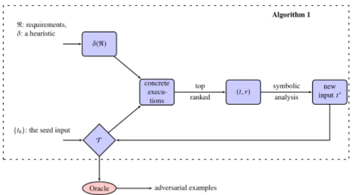
This section describes the overall design of the concolic testing ap-proach for requirements expressed using our formalism. The method alternates between concretely evaluating a DNN’s activation pat-terns and symbolically generating new inputs. The concolic testing pseudocode is in Algorithm1and the corresponding workflow is depicted in Figure1.
{t0}: the seed input T R: requirements, δ: a heuristic δ(R) concrete execu-tions (t,r) inputnewt′
Oracle adversarial examples
Algorithm 1
top ranked
symbolic analysis
Figure 1: Overview of our concolic testing method.
Algorithm1takes as inputs a DNNN, an inputt0, a heuristic
δ, and a setRof requirements, and produces a test suiteT. In the algorithm,tis the latest test case generated, and is initialised as the inputt0. For every test requirementr ∈ R, it is removed fromR
whenever satisfied byT, i.e.,T |=r.
Algorithm 1Concolic Testing Algorithm for DNNs
INPUT:N,R,δ,t0 OUTPUT:T 1: T ← {t0}andS={} 2: t←t0 3: whileR,∅do 4: foreachr∈Rdo 5: ifT |=rthen R←R\ {r} 6: whiletruedo 7: t,r←requirement_evaluation(T,δ(R)) 8: t′←symbolic_analysis(t,r)
9: if soundness_check(t′)=truethen
10: T ← T ∪ {t′} 11: break 12: else 13: S←S∪ {(t,r)} 14: if S=T ×Rthen returnT 15: returnT
The functionrequirement_evaluation(Line 7), whose details are given in Section7, aims to find a pair(t,r)2of input and requirement 2For some requirements, we might return two inputst
1andt2. Here, for simplicity, we describe the case for a single input. The generalisation to two inputs is straightforward.
which, according to our concrete evaluation, are the most promising in finding a new test caset′to satisfy the requirementr. The heuristic δis a transformation function mapping a quantified formularwith operator∃into an optimisation formulaδ(r)with operatorargopt. In the evaluation, concrete executions are applied.
After obtaining(t,r), thesymbolic_analysis(Line 8), whose de-tails are in Section8, is applied to have a new concrete inputt′. Then a functionsoundness_check(Line 9), whose details are given in Section9, is applied to check if the new input is sound or not. The setSmaintains a set of(t,r)pairs on which our symbolic analysis cannot find a sound new input.
The algorithm has two termination conditions. When all test requirements inRhave been satisfied, i.e.,R = ∅, or no further requirement inRcan be satisfied, i.e.,S =T ×R, the algorithm terminates and returns the current test suiteT.
As shown in Figure1, after the generation of test suiteT by Algorithm1,Twill run through an oracle, i.e.,robustness_oracle in Section9, in order to evaluate the robustness of the DNN.
7
REQUIREMENT EVALUATION
This section presents our approach for Line 7 of Algorithm1. Given a set of requirementsRthat have not been satisfied, a heuristicδ, and the current setT of test cases, the goal is to select a concrete inputt∈ Ttogether with a requirementr∈R, both of which will be used later in a symbolic approach to find the next concrete input t′
(to be given in Section8). The selection oft andris done by concrete executions.
The general idea of obtaining(t,r)is as follows. For all require-mentsr∈R, we transformrintoδ(r)by utilising operatorsargopt
foropt∈ {max,min}that will be evaluated by concretely executing tests inT. AsRmay contain more than one requirement, we return the pair(t,r)such that
r=arg max
r {val(t,δ(r)) |r∈R}. (16)
Note that, when evaluatingargoptformulas (e.g.,arg minxa:e),
if an inputt ∈ Tis returned, we may need the value (minxa:e)
as well. We useval(t,δ(r))to denote such a value for the returned inputtand the requirement formular.
The formulaδ(r)expresses an optimisation objective together with a set of constraints. We will give several examples later in Sec-tion7.1. In the following, we extend the semantics in Definition4.3 to work with formulas withargoptoperators foropt∈ {max,min}, includingargoptxa:eandargoptx1,x2a:e. Intuitively,arg maxxa: e(arg minxa:e, resp.) is to find the inputxamong those
satisfy-ing Boolean formulae to maximise (minimise) the value of the arithmetic formulaa. Formally,
•the evaluation ofarg minxa:eonT returns an inputt ∈ T
such that,T |=e[x 7→t]and for allt′∈ T such thatT |= e[x 7→t′]we havea[x 7→t] ≤a[x 7→t′].
•the evaluation ofT |=arg minx1,x2a:eonT returns two inputst1,t1∈ Tsuch that,T |=e[x17→t1][x27→t2]and for
allt1′,t2′∈ T such thatT |=e[x1 7→t′
1][x27→t
′
2]we have
a[x17→t1][x27→t2] ≤a[x17→t1′][x27→t2′].
The cases forarg maxformulas are similar to those for arg min, by replacing≤with≥. Similarly to Definition4.3, the semantics is for a setT of test cases and we can adapt it to work with an
input subspaceX ⊆DL
1. We remark that in concrete execution the evaluation is onT.
7.1
Heuristics
For the several requirementsrdiscussed in Section5, we present the formulaδ(r)used in this paper. We remark that, sinceδis a heuristic, there exist other definitions. The following definitions work well in our experiments.
7.1.1 Lipschitz Continuity.When a Lipschitz requirementras in Equation (11) is unsatisfiable onT, we transform it intoδ(r)as follows:
arg max
x1,x2
.||v[x1]1−v[x2]1|| −c∗ ||x1−x2||:x1,x2∈X (17)
According to the semantics in Definition4.3, the aim is to find the bestt1andt2fromT to make the evaluation of||v[t1]1−v[t2]1|| −
c∗ ||t1−t2||as large as possible. As described, we also need to
computeval(t1,t2,r)=||v[t1]1−v[t2]1|| −c∗ ||t1−t2||.
7.1.2 Neuron Cover.When a requirementrin Equation (12) is unsatisfiable onT, we transform it into the following requirement δ(r):
arg max
x ck·uk,i[x]:true (18)
According to the semantics, the requirement will return the input t ∈ Tthat has the maximal value forck·uk,i[x].
The coefficientck is a layer-wise constant. It is based on the
following observation. With the propagation of signals in the DNN, activation values at each layer can be of different magnitudes. For example, if the minimum activation value of neurons at layerk andk+1are -10 and -100 respectively, then even when a neuron u[x]k,i =−1>−2=u[x]k+1,j, we may still regardnk+1,jas being closer to be activated thanuk,iis. Consequently, we define a layer
factorck for each layer which normalises the average activation
valuations of neurons at different layers into the same magnitude level. It is estimated by sampling a large enough input dataset.
7.1.3 SS Cover.In the SS Cover, given a decision neuronnk+1,j, the concrete evaluation aims to select one of its condition neurons nk,iat layerksuch that, for the test case to be generated, the signs
ofnk,i andnk+1,jcan be negated and the rest ofnk+1,j’s condition neurons reserve their respective signs. This is achieved by having the followingδ(r):
arg max
x −ck· |u[x]k,i|:true (19)
Intuitively, given the decision neuronnk+1,j, Equation (19) selects
the condition that is closest to the change of activation sign (i.e., smallest|u[x]k,i|).
7.1.4 Neuron Boundary Cover.We transform the requirementr in Equation (20) into the followingδ(r)when it is not satisfiable on
T; it selects the neuron that is closest to either the higher or lower boundary.
arg maxxck· (u[x]k,i−hk,i):true
arg maxxck· (lk,i−u[x]k,i):true
8
SYMBOLIC GENERATION OF NEW
CONCRETE INPUTS
This section presents our approach for Line 8 of Algorithm1. That is, given a concrete inputt and a requirementr, we need to find the next concrete inputt′by symbolic analysis. This newt′will be added into the test suite, i.e., Line 10 of Algorithm1. The symbolic analysis techniques to be considered include the linear programming method in [23], a global optimisation method for theL0norm in
[21], and a new optimisation algorithm to be introduced below. We regard optimisation algorithms as symbolic analysis methods because, similarly to constraint solving methods, they work with a set of test cases in a single run.
Thanks to the use ofDR, for each symbolic analysis method, its application to different test criteria can be formulated under a unified logic framework. To ease the presentation, the following description may, for each algorithm, focus on a few requirements, but we remark that all algorithms can work with all the requirements given in Section5.
8.1
Symbolic Analysis using Linear Programming
As explained in Section4, given an inputx, the DNN instanceN [x]maps to an activation patternap[x]that can be modeled us-ing Linear Programmus-ing (LP). In particular, the followus-ing linear constraints [23] yield a set of inputs that exhibit the same ReLU behaviour asx: {uk,i= Õ 1≤j≤sk−1 {wk−1,j,i·vk−1,j}+bk,i|k∈ [2,K],i∈ [1..sk]} (21) {uk,i≥0∧uk,i=vk,i|ap[x]k,i=true,k∈ [2,K),i∈ [1..sk]} ∪{uk,i<0∧vk,i=0|ap[x]k,i=false,k∈ [2,K),i∈ [1..sk]} (22)
Real valued variablesin the LP model are emphasized inbold.
•The activation value of each neuron is encoded by the linear constraint in (21), which is a symbolic version of the Equation (2) that calculates a neuron’s activation.
•Given a particular inputx, the activation pattern (Definition 4.1)ap[x]is known, withap[x]k,ibeing eithertrueorfalse that represents the ReLU’s activation or not for the neuron nk,i. Following the definition of ReLU in (1), for every
neu-ronnk,i, the linear constraints in (22) encode its ReLU’s activation (when ap[x]k,i = true) or deactivation (when ap[x]k,i =false).
The linear model (denoted asCfor generic purposes) given by (21) and (22) represents an input set that results in the same acti-vation pattern as encoded. Consequently, the symbolic analysis for finding a new inputt′from a pair(t,r)of input and requirement is equivalent to finding a new activation pattern.Note that, to make sure that the obtained test case is meaningful, in the LP model an objective is added to minimize the distance betweentandt′.Thus, the use of LP requires that a distance metric be linear, e.g.,L∞-norm in (6).
8.1.1 Neuron Coverage.The symbolic analysis of neuron cov-erage takes the input test casetand requirementr, let us say, on the activation of neuronnk,i, and it shall return a new testt′such that the test requirement is satisfied by the network instanceN [t′]. As a result, givenN [t]’s activation patternap[t], we can build up a new
activation patternap′such that
{ap′ k,i=¬ap[t]k,i∧∀k1<k: Û 0≤i1≤sk1 ap′ k1,i1=ap[t]k1,i1} (23) This activation pattern specifies the following conditions.
•nk,i’s activation sign is negated: this ensures the aim of the symbolic analysis to activatenk,i.
• In the new activation patternap′, the neurons before layer kpreserve their activation signs as inap[t]. Though there may exist various activation patterns that makenk,i activated,
for the use of LP modeling one particular combination of activation signs must be pre-determined.
• Other neurons are irrelevant, as the sign ofnk,i is only af-fected by the activation values of those neurons in previous layers.
Finally, the new activation patternap′defined in (23) is encoded by the LP modelCusing (21) and (22), and if there exists a feasible solution, then it will become the new test caset′, which makes the DNN satisfy the requirementr.
8.1.2 SS Coverage. When it comes to SS Coverage, to satisfy the requirementrwe need to find a new test case such that, with respect to the inputt, activation signs ofnk+1,jandnk,i are negated,
while other signs of other neurons at layerkare kept the same as in the case of inputt. To achieve this, the following activation pattern ap′is built up for the LP modeling.
{ap′ k,i =¬ap[t]k,i ∧ap ′ k+1,j=¬ap[t]k+1,j ∧∀k1<k: Ó 1≤i1≤sk1 ap′ k1,i1=ap[t]k1,i1}
8.1.3 Neuron Boundary Coverage.In case of the neuron bound-ary coverage, the symbolic analysis aims to find an inputt′such that the neuronnk,i’s activation value exceeds either its higher bound hk,i or its lower boundlk,i. To achieve this, while preserving the
DNN activation pattern asap[t], we add one of the following con-straints into the LP program.
• Ifu[x]k,i−hk,i >lk,i−u[x]k,i:uk,i>hk,i; • otherwise:uk,i<lk,i.
8.2
Symbolic Analysis using Global Optimisation
The symbolic analysis for finding a new input can also be imple-mented by solving the global optimisation problem in [21]. That is, by specifying the test requirement as an optimisation objective, we apply global optimisation to find a test case that makes the test requirement satisfied. Readers are referred to [21] for the details of the algorithm.• For Neuron Coverage, the objective is thus to find at′such that the specified neuronnk,ihasap[t′]k,i =true.
• In case of SS Coverage, given the neuron pair(nk,i,nk+1,j)
and the original inputt, the optimisation objective becomes ap[t′]k,i ,ap[t]k,i∧ap[t′]k+1,j,
ap[t]k+1,j∧ Ó i′
,i
ap[t′]k,i′=ap[t]k,i
• Regarding the Neuron Boundary Coverage, depending on whether the higher bound or lower bound for the activation ofnk,i is considered, the objective of finding a new input
t′can be one of the two forms: 1)u[t′]
k,i > hk,i or 2) u[t′]k,i <lk,i.
8.3
Lipschitz Test Case Generation
Given a requirement in Equation (11) for a subspaceX, we let t0∈Rn be the representative point of the subspaceX to whicht1
andt2belong. The optimisation problem is to generate two inputst1
andt2such that
||v[t1]1−v[t2]1||D
1−c∗ ||t1−t2||D1 >0
s.t.||t1−t0||D2 ≤∆, ||t2−t0||D2 ≤∆ (24)
where|| ∗ ||D
1 and|| ∗ ||D2 denote certain norm metrics such as
theL0-norm,L2-norm orL∞-norm, and∆intuitively represents the radius of a norm ball (forL1,L2-norm) or the size of a hypercube (for
L∞-norm) centered ont0.∆is a hyper-parameter of the algorithm.
The above problem can be efficiently solved by a novel alternat-ing compass searchscheme. Specifically, we alternately optimise the following two optimisation problems through relaxation [19], i.e., maximizing the lower bound of the original Lipschitz constant instead of directly maximizing the Lipschitz constant itself. To do so we formulate the original non-linear proportional optimisation as a linear problem when both norm metrics|| ∗ ||D1and|| ∗ ||D2are L∞-norm.
8.3.1 Stage One.We solve
min t1 F(t1,t0)=−||v[t1]1−v[t0]1||D1 s.t.||t1−t0||D 2≤∆ (25) The above objective enables the algorithm to search for an optimalt1
in the space of a norm ball or hypercube centered ont0with radius∆,
such that the norm distance ofv[t1]1andv[t0]1is as large as possible. From the constraint, we know thatsup| |t1−t0| |D2≤∆||t1−t0||D2 =
∆. Thus a smallerF(t1,t0)essentially leads to a larger Lipschitz constant, considering thatLip(t1,t0) = −F(t1,t0)/||t1−t0||D
2 ≥ −F(t1,t0)/∆, i.e.,−F(t1,t0)/∆is the lower bound ofLip(t1,t0). There-fore, the searching trace of minimizingF(t1,t0)will generally lead to an increase of the Lipschitz constant.
To solve the above the problem we use the compass search method [2], which is efficient, derivative-free, and guaranteed to have first-order global convergence. Because we aim to find an input pair to break the predefined Lipschitz constantcinstead of finding the largest Lipschitz constant, along each iteration, when we gett¯1,
we check whetherLip(t¯1,t0)>c. If it holds, we find an input pair
¯
t1andt0that satisfies the test requirement; otherwise, we continue
the compass search until convergence or a satisfiable input pair is generated. If Equation (25) is convergent and we can find an optimal t1as
t∗
1 =arg mint
1
F(t1,t0)s.t.||t1−t0||D2≤∆
but we still cannot find a satisfiable input pair, we perform Stage Two optimisation.
8.3.2 Stage Two.We solve
min t2 F(t1∗,t2)=−||v[t2]1−v[t∗1]1||D1 s.t.||t2−t0||D 2≤∆ (26) Similarly, we use derivative-free compass search to solve the above problem and check whetherLip(t1∗,t2) >cholds at each iterative
optimisation tracet¯2. If it holds, we return the image pairt∗1and
¯
t2 that satisfies the test requirement; otherwise, we continue the
optimisation until convergence or a satisfiable input pair is generated. If Equation (26) is convergent att2∗, and we still cannot find such a input pair, we modify the objective function again by lettingt1∗=t∗2 in Equation (26) and continue the search and satisfiability checking procedure.
8.3.3 Stage Three.If the functionLip(t∗
1,t
∗
2)stops increasing
in Stage Two, we treat the whole search procedure as convergent and fail to find an input pair that can break the predefined Lipschitz constantc. In this case, we return the best input pair we can find, i.e., t∗
1andt2∗, and the largest Lipschitz constantLip(t1∗,t2). Note that the
returned constant is smaller thanc.
In summary, the proposed method is an alternating optimisation scheme based on the compass search. Basically, we start from the givent0to search for an imaget1in a norm ball or hypercube, where
the optimisation trajectory on the norm ball space is denoted as S(t0,∆(t0))) such thatLip(t0,t1) >c(this step is symbolic execu-tion); if we cannot find it, we modify the optimisation objective function by replacingt0witht1∗(the best concrete input found in
this optimisation trace) to initiate another optimisation trajectory on the space, i.e.,S(t∗
1,∆(t0)). This process is repeated until the
optimi-sation trace gradually covers the whole norm ball spaceS(∆(t0)).
9
ORACLE
First of all, we provide details to Line 10 of Algorithm1about the soundness checking.
Definition 9.1 (Soundness Checking). Given a setOof correctly classified inputs (e.g., the training dataset) and a real numberb, a test caset′∈ Tpasses the soundness checking if
∃t∈O: ||t−t′|| ≤b (27)
Intuitively, it says that the test casetis sound if it is close to some of the correctly classified inputs inO. Given a test caset′∈ T, we can writeO(t′)for the inputt ∈Owhich has the smallest distance tot′among all inputs inO.
When checking the quality of the generated test suiteT, we use the following oracle.
Definition 9.2 (Robustness Oracle). Given a setOof correctly classified inputs, a test caset′passes the robustness oracle if
arg maxjv[t′]K,j =arg maxjv[O(t′)]K,j (28)
Intuitively, the role of this oracle is to check the robustness of the DNN on inputO(t′): ift′cannot pass the oracle then it serves as evidence of the DNN lacking in robustness.
10
A SUMMARY OF COVERAGE-BASED DNN
TESTING
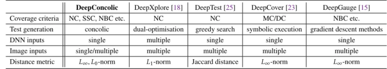
We briefly summarise the similarities and differences between our concolic testing method, namedDeepConcolic, and other existing coverage-driven DNN testing methods: DeepXplore [18], DeepTest [25], DeepCover [23], and DeepGauge [15]. The details are pre-sented in Table1, where NC, SSC, and NBC are short for Neuron Cover, SS Cover, and Neuron Boundary Cover, respectively. In addition to the concolic nature of DeepConcolic, we observe the following differences.
Table 1: Comparison between different coverage-based DNN testing methods
DeepConcolic DeepXplore [18] DeepTest [25] DeepCover [23] DeepGauge [15]
Coverage criteria NC, SSC, NBC etc. NC NC MC/DC NBC etc.
Test generation concolic dual-optimisation greedy search symbolic execution gradient descent methods
DNN inputs single multiple single single single
Image inputs single/multiple multiple multiple multiple multiple Distance metric L∞,L0-norm L1-norm Jaccard distance L∞-norm L∞-norm
•DeepConcolic is generic, using a unified language DR to express test requirements and a small set of algorithms to compute a class of requirements; the other methods aread hoctests for specific requirements.
•Comparing with DeepXplore, which needs a set of DNNs to explore multiple gradient directions, the other methods, including DeepConcolic, need a single DNN only.
•In contrast to the other methods, DeepConcolic can achieve good coverage by starting from a single input; the other meth-ods need a non-trivial set of inputs.
•Until now, there is no conclusion on the best distance metric. DeepConcolic can be parameterized with a desired norm distance metric|| · ||.
Moreover, from the workflow given in Figure1, we can see that DeepConcolic features a clean separation between the generation of test cases and the oracle. This is well aligned with the traditional approach to test case generation. The other methods essentially use the oracles of Section9as part of their objectives to guide the generation of test cases.
11
EXPERIMENTAL RESULTS
The concolic testing approach presented in this paper has been implemented in a software tool we have named DeepConcolic3. In this section, we compare it with the latest DNN testing tools and evaluate its performance for different test requirements. The experiments are run on a machine with 24 cores Intel(R) Xeon(R) CPU E5-2620 v3 @ 2.40GHz and 125G memory. When testing a DNN, if the DeepConcolic testing does not finish within 12 hours, it is forced to terminate. All coverage results are collected by running the testing repeatedly at least 10 times.
11.1
Comparison with DeepXplore
This section compares the use of DeepConcolic and DeepXplore [18] for two state-of-the-art DNNs on the MNIST and CIFAR-10 datasets, respectively. We remark that DeepXplore has been tested on further datasets.
For each tool, we start neuron cover testing from a randomly sampled image input. Note that, since DeepXplore requires more than one DNN, we designate our trained DNN as the target model and utilise the other two default models provided by DeepXplore. Table2gives the neuron cover reports from the two tools. We ob-serve that DeepConcolic yields much higher neuron coverage than
3The implementation and all data in this section are available online at
https://github.com/TrustAI/DeepConcolic
DeepXplore in any of its three modes of operation (‘light’, ‘occlu-sion’, and ‘blackout’). On the other hand, DeepXplore is much faster and terminates in seconds.
Table 2: Neuron coverage of DeepConcolic and DeepXplore
DeepConcolic DeepXplore
L∞-norm L0-norm light occlusion blackout
MNIST 97.60% 95.91% 80.77% 82.68% 81.61%
CIFAR-10 84.98% 98.63% 77.56% 81.48% 83.25%
Figure 2: Adversarial images of DNNs, with L∞-norm for
MNIST (top row) andL0-norm for CIFAR-10 (bottom row),
generated by DeepConcolic and DeepXplore, the latter with im-age constraints ‘light’, ‘occlusion’, and ‘blackout’.
Figure2exhibits several adversarial examples found by DeepCon-colic (withL∞-norm andL0-norm) and DeepXplore. It is worth
not-ing that, although DeepConcolic does not impose particular domain-specific constraints on the original image as DeepXplore does, the concolic testing procedure generates test cases that resemble “human perception”. For example, based on theL∞-norm, it produces adver-sarial examples (Figure2, top row) that gradually reverse the black and white colours. For theL0-norm, DeepConcolic generates
adver-sarial examples similar to those of DeepXplore under the ‘blackout’ constraint, which is essentially pixel manipulation.
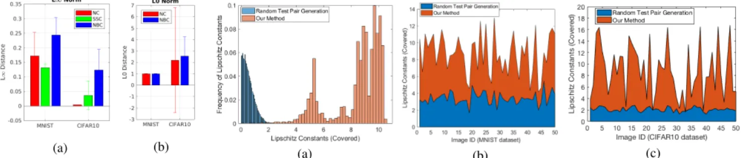
0.2 0.4 0.6 0.8 1 1.2 MNIST CIFAR-10 Coverage NC SSC NBC (a)L∞-norm 0.2 0.4 0.6 0.8 1 1.2 MNIST CIFAR-10 Coverage NC NBC (b)L0-norm
(a) (b)
Figure 4: (a) Distance of NC, SSC, and NBC on MINIST and
CIFAR-10 datasets based on L∞ norm;
(b) Distance of NC and NBC on the
two datasets based onL0norm.
(a) (b) (c)
Figure 5: (a) Lipschitz Constant Coverage generated by 1,000,000 randomly generated test pairs and our concolic testing method for input image-1 on MNIST DNN; (b) Lipschitz Con-stant Coverages generated by random testing and our method for 50 input images on MNIST DNN; (c) Lipschitz Constant Coverage generated by random testing and our method for 50 input images on CIFAR-10 DNN.
11.2
Testing Results on Different Test Criteria
This section presents the results of applying DeepConcolic to evalu-ate the test criteria NC, SSC, and NBC. DeepConcolic starts the NC testing with one single seed input. For SSC and NBC, to improve the performance, an initial set of 1000 images are sampled. Furthermore, for experimental purposes, we only test a subset of the neurons for SSC and NBC. A distance upper bound of 0.3 (L∞-norm) and 100 pixels (L0-norm) is set up for collecting adversarial examples.The full coverage report, including the average coverage and stan-dard derivation, is given in Figure3. Table3contains the adversarial example results. We have observed that the overhead for the sym-bolic analysis based on global optimisation in Section8.2is too high. Thus, the SSC result withL0-norm is excluded.
Table 3: Adversarial examples by different test criteria, dis-tance metrics, and DNN models
L∞-norm L0-norm MNIST CIFAR-10 MNIST CIFAR-10
adversary /test suite minimum distance adversary /test suite minimum distance adversary /test suite minimum distance adversary /test suite minimum distance NC 13.93% 0.0039 0.79% 0.0039 0.53% 1 5.59% 1 SSC 0.02% 0.1215 0.36% 0.0039 – – – – NBC 0.20% 0.0806 7.71% 0.0113 0.09% 1 4.13% 1
Overall, DeepConcolic achieves high coverage and, according to the robustness check in Definition9.2, detects a significant portion of adversarial examples, with the cover of corner-case activation values (i.e., NBC) sometimes being harder to achieve.
Concolic testing is able to find adversarial examples with the minimum possible distance: that is,2551 ≈0.0039for theL∞norm and1pixel for theL0norm. Figure4gives the average distance of
adversarial examples (from one DeepConcolic run), which often falls into a reasonably small distance range. Remarkably, for the same network, the number of adversarial examples found under the NC can be quite different when the distance metric is changed. This observation suggests that, when designing test criteria for DNNs, they need to be examined using different distance metrics.
11.3
Results for Lipschitz Constant Testing
This section reports experimental results for the Lipschitz con-stant testing on DNNs. We test Lipschitz concon-stants ranging over
{0.01 : 0.01 : 20}on 50 MNIST images and 50 CIFAR-10 images respectively. Every image represents a subspace inDL1and thus a requirement in Equation (11).
11.3.1 Baseline Method.Since this paper is the first to test Lips-chitz constants of DNNs, we compare our method with random test case generation. For this specific test requirement, given a predefined Lipschitz constantc, an inputt0and the radius of norm ball (e.g., for
L1andL2norms) or hypercube space (forL∞-norm)∆, we randomly generate two test pairst1andt2that satisfy the space constraint (i.e.,
||t1−t0||D
2 ≤ ∆and||t2−t0||D2 ≤ ∆), and then check whether Lip(t1,t2)>cholds. We repeat the random generation until we find
a satisfying test pair or the number of repetitions is larger than a predefined threshold. We set such threshold asNr d =1,000,000.
Namely, if we randomly generate 1,000,000 test pairs and none of them can satisfy the Lipschitz constant requirement>c, we treat this test as a failure and return the largest Lipschitz constant found and the corresponding test pair; otherwise, we treat it as successful and return the satisfying test pair.
11.3.2 Experimental Results.Figure5(a) depicts the Lipschitz Constant Coverage generated by 1,000,000 random test pairs and our concolic test generation method for image-1 on MNIST DNNs. As we can see, even though we produce 1,000,000 test pairs by random test generation, the maximum Lipschitz converage reaches only 3.23 and most of the test pairs are in the range[0.01,2]. Our concolic method, on the other hand, can cover a Lipschitz range of[0.01,10.38], where most cases lie in[3.5,10], which is poorly covered by random test generation.
Figure5(b) and (c) compare the Lipschitz constant coverage of test pairs from the random method and the concolic method on both MNIST and CIFAR-10 models. Our method significantly outperforms random test case generation. We note that covering a large Lipschitz constant range for DNNs is a challenging problem since most image pairs (within a certain high-dimensional space) can produce small Lipschitz constants (such as 1 to 2). This ex-plains the reason why randomly generated test pairs concentrate in a range of less than 3. However, for safety-critical applications such as self-driving cars, a DNN with a large Lipschitz constant essentially indicates it is more vulnerable to adversarial perturbations [20,21].
As a result, a test method that can cover larger Lipschitz constants provides a useful robustness indicator for a trained DNN. We argue that, for safety testing of DNNs, the concolic test method for Lips-chitz constant coverage can complement existing methods to achieve significantly better coverage.
12
CONCLUSIONS
In this paper, we propose the first concolic testing method for DNNs. We implement it in a software tool and apply the tool to evaluate DNN robustness, through coverage testing for Lipschitz continuity and several other test criteria. Experimental results confirm that the combination of concrete execution and symbolic analysis serves as a viable approach for DNN testing.
REFERENCES
[1] Martin Arjovsky, Soumith Chintala, and Léon Bottou. 2017. Wasserstein GAN.
arXiv preprint arXiv:1701.07875(2017).
[2] Charles Audet and Warren Hare. 2017.Derivative-Free and Blackbox Optimiza-tion. Springer.
[3] Radu Balan, Maneesh Singh, and Dongmian Zou. 2017. Lipschitz Properties for Deep Convolutional Networks.arXiv preprint arXiv:1701.05217(2017). [4] Jacob Burnim and Koushik Sen. 2008. Heuristics for Scalable Dynamic Test
Gen-eration. InAutomated Software Engineering, ASE. 23rd International Conference on. IEEE, 443–446.
[5] Cristian Cadar, Daniel Dunbar, Dawson R Engler, and others. 2008. KLEE: Unas-sisted and Automatic Generation of High-Coverage Tests for Complex Systems Programs.. InOSDI, Vol. 8. 209–224.
[6] Sooyoung Cha, Seongjoon Hong, Junhee Lee, and Hakjoo Oh. 2018. Automati-cally Generating Search Heuristics for Concolic Testing. InProceedings of the 40th International Conference on Software Engineering. ACM, 1244–1254. [7] Timon Gehr, Matthew Mirman, Dana Drachsler-Cohen, Petar Tsankov, Swarat
Chaudhuri, and Martin Vechev. 2018. AI2: Safety and Robustness Certification of Neural Networks with Abstract Interpretation. InSecurity and Privacy (SP), 2018 IEEE Symposium on.
[8] Patrice Godefroid, Nils Klarlund, and Koushik Sen. 2005. DART: Directed Automated Random Testing. InProceedings of the ACM SIGPLAN Conference on Programming Language Design and Implementation. 213–223.
[9] Patrice Godefroid, Michael Y Levin, David A Molnar, and others. 2008. Auto-mated Whitebox Fuzz Testing. InNDSS, Vol. 8. 151–166.
[10] Kelly Hayhurst, Dan Veerhusen, John Chilenski, and Leanna Rierson. 2001.
A Practical Tutorial on Modified Condition/Decision Coverage. Technical Report. NASA.
[11] Xiaowei Huang, Marta Kwiatkowska, Sen Wang, and Min Wu. 2017. Safety Verification of Deep Neural Networks. InInternational Conference on Computer Aided Verification. Springer, 3–29.
[12] Cem Kaner. 2006. Exploratory Testing. InQuality Assurance Institute Worldwide Annual Software Testing Conference.
[13] Raghudeep Kannavara, Christopher J Havlicek, Bo Chen, Mark R Tuttle, Kai Cong, Sandip Ray, and Fei Xie. 2015. Challenges and Opportunities with Concolic Testing. InAerospace and Electronics Conference (NAECON), 2015 National. IEEE, 374–378.
[14] Guy Katz, Clark Barrett, David L Dill, Kyle Julian, and Mykel J Kochenderfer. 2017. Reluplex: An Efficient SMT Solver for Verifying Deep Neural Networks.
InInternational Conference on Computer Aided Verification. Springer, 97–117. [15] Lei Ma, Felix Juefei-Xu, Jiyuan Sun, Chunyang Chen, Ting Su, Fuyuan Zhang,
Minhui Xue, Bo Li, Li Li, Yang Liu, and others. 2018. DeepGauge: Comprehen-sive and Multi-Granularity Testing Criteria for Gauging the Robustness of Deep Learning Systems.arXiv preprint arXiv:1803.07519(2018).
[16] Matthew Mirman, Timon Gehr, and Martin Vechev. 2018. Differentiable Abstract Interpretation for Provably Robust Neural Networks. InInternational Conference on Machine Learning. 3575–3583.
[17] Vinod Nair and Geoffrey E Hinton. 2010. Rectified Linear Units Improve Re-stricted Boltzmann Machines. InInternational Conference on Machine Learning. 807–814.
[18] Kexin Pei, Yinzhi Cao, Junfeng Yang, and Suman Jana. 2017. DeepXplore: Automated Whitebox Testing of Deep Learning Systems. InProceedings of the 26th Symposium on Operating Systems Principles. ACM, 1–18.
[19] T. Roubicek. 1997.Relaxation in Optimization Theory and Variational Calculus. Berlin: Walter de Gruyter.
[20] Wenjie Ruan, Xiaowei Huang, and Marta Kwiatkowska. 2018. Reachability Anal-ysis of Deep Neural Networks with Provable Guarantees.The 27th International Joint Conference on Artificial Intelligence (IJCAI)(2018).
[21] Wenjie Ruan, Min Wu, Youcheng Sun, Xiaowei Huang, Daniel Kroening, and Marta Kwiatkowska. 2018. Global Robustness Evaluation of Deep Neural Net-works with Provable Guarantees for L0 Norm.arXiv preprint arXiv:1804.05805v1
(2018).
[22] Koushik Sen, Darko Marinov, and Gul Agha. 2005. CUTE: A Concolic Unit Testing Engine for C.ACM SIGSOFT Software Engineering Notes30, 5 (2005), 263–272.
[23] Youcheng Sun, Xiaowei Huang, and Daniel Kroening. 2018. Testing Deep Neural Networks.arXiv preprint arXiv:1803.04792(2018).
[24] Christian Szegedy, Wojciech Zaremba, Ilya Sutskever, Joan Bruna, Dumitru Erhan, Ian Goodfellow, and Rob Fergus. 2014. Intriguing Properties of Neural Networks. InInternational Conference on Learning Representations (ICLR).
[25] Yuchi Tian, Kexin Pei, Suman Jana, and Baishakhi Ray. 2018. DeepTest: Auto-mated Testing of Deep-Neural-Network-Driven Autonomous Cars. InProceedings of the 40th International Conference on Software Engineering. ACM, 303–314. [26] Willem Visser, Corina S PÇ ˝OsÇ ˝Oreanu, and Sarfraz Khurshid. 2004. Test Input
Generation with Java PathFinder.ACM SIGSOFT Software Engineering Notes29, 4 (2004), 97–107.
[27] Xinyu Wang, Jun Sun, Zhenbang Chen, Peixin Zhang, Jingyi Wang, and Yun Lin. 2018. Towards Optimal Concolic Testing. InProceedings of the 40th International Conference on Software Engineering. ACM, 291–302.
[28] Zhou Wang, Eero P Simoncelli, and Alan C Bovik. 2003. Multiscale Structural Similarity for Image Quality Assessment. InSignals, Systems and Computers, Conference Record of the Thirty-Seventh Asilomar Conference on.
[29] Thomas Wiatowski and Helmut Bölcskei. 2018. A Mathematical Theory of Deep Convolutional Neural Networks for Feature Extraction. IEEE Transactions on Information Theory64, 3 (2018), 1845–1866.
[30] Matthew Wicker, Xiaowei Huang, and Marta Kwiatkowska. 2018. Feature-Guided Black-Box Safety Testing of Deep Neural Networks. InInternational Conference on Tools and Algorithms for the Construction and Analysis of Systems. Springer, 408–426.
[31] Min Wu, Matthew Wicker, Wenjie Ruan, Xiaowei Huang, and Marta Kwiatkowska. 2018. A Game-Based Approximate Verification of Deep Neural Networks with Provable Guarantees.arXiv preprint arXiv:1807.03571(2018).
[32] Tao Xie, Darko Marinov, Wolfram Schulte, and David Notkin. 2005. Symstra: A Framework for Generating Object-Oriented Unit Tests using Symbolic Execu-tion. InInternational Conference on Tools and Algorithms for the Construction and Analysis of Systems (LNCS), Vol. 3440. Springer, 365–381.