DAM BREAK FLOW SIMULATION ON GRID

DAM BREAK FLOW SIMULATION ON GRID

1 _{Laboratory of Parallel Computing, Vilnius Gediminas Technical University,} Saulėtekio 11, LT-10223, Vilnius, Lithuania

2 _{Computing Centre, Vilnius Gediminas Technical University,} Saulėtekio 11, LT-10223, Vilnius, Lithuania

*E-mail: [email protected]

Abstract. In this contribution we report on a dam break flow simulation on gLite based grid infrastructure. The dam break problem including breaking waves is solved by the pseudo-concentration method improved by interface sharpening technique. The developed interface sharpening procedure helps to preserve interface sharpness and mass conservation. The com-puted position of the leading edge of water column has been compared with the experimental measurements.

1. Introduction

Dam break flow has been the subject of extensive research for a long time [1]. The original problem has direct application in the industrial areas of fluid mechanics and environment pro-tection. The breaking wave phenomena occurring in some cases of a dam break problem in-cludes it into the class of complex applications such as solitary wave propagation, tank slosh-ing and water on a ship deck simulation. Some experimental measurements were performed on the dam break flow or collapse of a liquid column problem [1-2]. Photographs showing the time evolution of the collapsing column as well as the wave returning after hitting a wall on the opposite side are available for the purpose of evaluating the numerical methodology on the basis of flow visualization. Measurements of the exact interface shape are not available, but some secondary data such as the reduction of the water column height [2] can be em-ployed for quantitative comparison of the obtained results. Several modifications of the bro-ken dam problem have been extensively used as classical test cases for numerical simulation of free surfaces and moving interfaces [3-4]. However, the universal, accurate and efficient numerical technique for breaking wave simulation attracts close attention of research com-munity and software developers.

Over the past 30 years, researchers have put a lot of effort into developing various nu-merical methods to simulate the moving interface flows governed by the Navier-Stokes equa-tions. All numerical methods for modelling of the moving interface flows are based on inter-face tracking approach or interinter-face capturing approach. In former, the liquid region is subdi-vided by a mesh, while each cell is deformed according to the movement of the interface and computed velocities [5-6]. However, this approach requires remeshing procedures to avoid of computation failure due to serious distortion of cells or elements. These methods are unable to cope naturally with interface interacting with itself by folding or rupturing. In the interface capturing approach, the mesh remains fixed and moving interface can not be directly defined by the mesh nodes. Therefore, additional technique is necessary to define the areas occupied by fluid or gas on either side of the interface. The marker-and-cell method [3], the volume of fluid method [4] and the level set method [7] are well known methods using the interface

turing approach. These methods require no geometry manipulations after the mesh is gener-ated and can be applied to interfaces of a complex topology [8]. However, the location of the interface is not explicit and, sometimes, the appropriate boundary conditions cannot be pre-scribed with a required accuracy.

A pseudo-concentration method [9] often used with the finite element method (FEM) is an interesting alternative for the other interface capturing methods. This method uses a pseudo-concentration function defined in the entire domain and solves a hyperbolic equation to determine the moving interface [10]. In the most cases, the pseudo-concentration method is more efficient than the level set method, because it uses simpler front reconstruction tech-niques. The FEM has become a powerful tool for solving many scientific and engineering applications; therefore, the demand for further investigation of the ICT and implementation in commercial FEM codes is rapidly growing [11]. The main concerns with the interface captur-ing approach have been the extensive usage of computational resources and sustaincaptur-ing global mass conservation in long-time integrations [12]. It was observed that numerical diffusion introduces a normal motion proportional to the local curvature of the interface, which leads to non-physical mass transfer between the two fluids. The choice of the interface sharpening procedure, the numerical schema and numerical parameters remain state of the art problem.

In the present paper, the efficient interface sharpening procedure preserving mass conser-vation is applied to the complex dam break flow. Numerical experiments are carried out on gLite based BalticGrid infrastructure providing the necessary computational resources.

2. Mathematical model of the flow

The laminar and Newtonian flow of viscous and incompressible fluids is described by the Navier-Stokes equations in the Eulerian reference frame:

j ij i j i j i x F x u u t u ∂ ∂ + = ⎟ ⎟ ⎠ ⎞ ⎜ ⎜ ⎝ ⎛ ∂ ∂ + ∂ ∂ _ρ σ ρ , (1) 0 x u i i = ∂ ∂ , (2)

where are the velocity components; u_i ρ is the density; are the gravity force components

and i F ij σ is stress tensor ⎟ ⎟ ⎠ ⎞ ⎜ ⎜ ⎝ ⎛ ∂ ∂ + ∂ ∂ + − = i j j i ij ij x u x u pδ µ σ . (3)

Here µ is the dynamic viscosity coefficient, p is the pressure and δ_ij is Kronecker delta.

Slip boundary conditions for velocity are prescribed on rigid walls:

0 n

ui i= , (4)

here are the components of a unit normal vector. This is usual choice of boundary condi-tions used for modelling of moving interface flows. The zero stress boundary condicondi-tions are prescribed on the open upper boundary

i n 0 nj ij = σ . (5)

The reference pressure is prescribed on the upper wall. The zero initial conditions are pre-scribed for the equations (1-3) in the performed investigation.

The pseudo-concentration method [9] is developed for moving interface flows using the Eulerian approach and the interface capturing idea. The pseudo-concentration function ϕ

serves as a marker, identifying fluids A and B with densities ρA and ρB and viscosities µA

and µB. In this context, the density and viscosity are defined as: B

A (1 ϕ)ρ ρ

ϕ

B A (1 ϕ)µ µ

ϕ

ρ = + − , (7)

where ϕ =1 forfluid A and ϕ=0 for fluid B. The evolution of the interface is governed by

the time dependent convection equation: ⎟ ⎟ ⎠ ⎞ ⎜ ⎜ ⎝ ⎛ ∂ ∂ + ∂ ∂ j j x u t ϕ ϕ _{. (8)}

The velocity is obtained from the solution of the Navier-Stokes equations (1-3). The initial conditions defined on the entire solution domain should be prescribed for equation (8).

i u

The space-time Galerkin least squares (GLS) finite element method [5] is applied as a general-purpose computational approach to solve the partial differential equations (13, 8) with boundary conditions (45) applied. Equal order bilinear shape functions are used for both the pressure and velocity components as well as for the pseudo-concentration function. The stabilization nature of the formulation prevents numerical oscillation of incompressible flows when equal-order interpolation functions for velocity and pressure are used and preserves the consistency of the standard Galerkin method when adaptive remeshing is performed. The de-tailed description of variational formulation and stabilization parameters can be found in work [13].

3. Interface sharpening procedure

The standard Galerkin formulation of the FEM yields oscillatory solutions when applied to convection dominant problems in conjunction with classical time stepping algorithms. Con-ventional stabilization techniques add to the equation (8) artificial viscosity terms, introduc-ing numerical diffusion and reducintroduc-ing numerical oscillations. In practical application of the GLS stabilizing method to the complex problems governed by convective transport, some overshoots and undershoots are observed [13]. In order to apply the developed interface sharpening procedure, a simpler limiter should be implemented:

[ ]

[

min ϕ

]

ϕ = . (9)

It removes the overshoots and undershoots, preventing the numerical technique from unex-pected incorrect values and the loss of accuracy.

While the equation (8) moves the interface at a correct velocity, the pseudo-concentration function may become significantly influenced by the numerical diffusion after some period of time. It leads to interface smearing and problems with mass conservation. The pseudo-concentration function should be reconstructed in order to maintain interface sharpness. In this work, the values of the pseudo-concentration function ϕ are replaced by the values of the reconstructed function φ according to the following formula:

a a 1 c ϕ φ₌ − _, c 0≤ϕ≤ , (10) a a 1 ) 1 ( ) c 1 ( 1 ϕ φ= − − − − _, 1 c≤ϕ≤ , (11)

where the parameter c represents mass conservation level, while governs sharpness of the

moving interface. The implicit parameter indicates how often this procedure should be applied. Usually, the interface thickness tends to grow, occupying a wide band of finite ele-ments. Frequent application of the interface sharpening procedure (1011) with large values

easily resolves this problem, but it can distort the smoothness of the interface. The moving front can adapt to the FE mesh proceeding “staircases”. In this undesirable case, the accuracy of the interface capturing technique becomes directly limited by the mesh size. Thus, the val-ues of parameter , controlling interface sharpness, should be chosen very carefully.

a ns

a

ns

Mass conservation is a very important issue of the interface sharpening algorithm. Insig-nificant numerical errors, which result in slight non-physical mass transfer between the two fluids, may lead to significant errors in long-term time integration of the problem. In order to

overcome this difficulty and to preserve mass conservation, the values of coefficient c

should be computed considering precise mass distribution in the interface region. At any time, mass conservation for fluid A in the solution domain Ω can be described by the

for-mula:

∫

where M_A is the initial mass of the fluid A. The equation for determining c can be obtained

by substituting φ from formulas (1011) to equation (12). Assuming that a is given and

con-stant, the resulting equation for mass conservation can be written as follows: ϕ A A a 1 2 a 1 1c K (1 c) M M K − − − − = − , (13)

where coefficient K1 is defined on the narrow band of the moving interface 0≤ϕ≤c:

∫

Coefficient K2 is computed on the remaining part of the interface c≤ϕ≤1:

∫

Coefficient ϕ represents the current mass of the fluid

A

M A, defined by the values of the ϕ

function c≤ϕ≤1:

∫

Despite the fact that only one fluid is explicitly presented in equation (13), the described pro-cedure conserves mass for each fluid. In the solved problems, the fluid A is heavy (water),

while the fluid B is relatively light (air). A good starting value for is 0.5, which indicates

satisfactory mass conservation. The final values of c are obtained solving one-dimensional

non-linear equation (13). Modelling breaking waves and other extreme phenomena, the final value varies in a relatively wide range from 0.2 to 0.8 [14]. After determining and c,

equations (10-11) are satisfied at the node-level, and the new value of the pseudo-concentration function is used to resume computations.

c

c a

4. Software deployment in grid

The discussed numerical algorithms have been implemented in the code FEMTOOL [13], which allows implementation of any partial differential equation with minor expenses. Time dependent problems are solved using space-time finite elements. The order of shape functions is determined by input and is limited neither in space nor in time. A given transient problem can be solved in several implicit time steps from one time level to the other or in one single implicit step for all time levels. Space-time finite element integration in time and the high or-der shape functions generated automatically make FEMTOOL to be applicable to complex strongly coupled problems of interest.

Several times FEMTOOL software was deployed in gLite based grid. The gLite Work-load Management System (WMS) natively supports the submission of MPI jobs, which are jobs composed of a number of processes running on different Working Nodes (WN) in the same Computing Element (CE). However, this support is still experimental; therefore, run-ning MPI applications on the gLite grid requires significant hand-turun-ning for each site. Some time ago MPI services were very inconvenient for the clusters using distributed home file systems. It was necessary to transfer executable and data files from the governing WN (zero number assigned by MPI) to the other WNs, to implement additional checks for their pres-ence and to ensure that all result files were transferred back to the governing WN. Any im-plementation of MPI-2 standard was not supported. The first FEMTOOL deployment relied

on shell scripts consisted of approximately 100 lines and required long preparation time. Only experienced system administrator can prepare and test such scripts for new MPI applications.

Improved FEMTOOL gridification was based on the compilers g95 and gcc as well as on the OpenMPI implementation. FEMTOOL version 3.0 has been deployed in BalticGrid-II testbed by using SGM (Software Grid Manager) system. All software packages are installed in the predefined location, which is specified by content of $VO_BGTUT_SW_DIR variable.

After successful installation, the SGM marks the site in global grid information system as ca-pable of running this particular application. By use of this flag, called "a tag" the ordinary users may indicate which sites they want to use. The FEMTOOL tag is VO-balticgrid-A-ENG-FEMTOOL-3.0.

Recent efforts made in Interactive European Grid project (int.eu.grid) [15] improved situation. The MPI-START scripts were developed by the MPI working group containing members from int.eu.grid and EGEE. The increased portability and flexibility was achieved by working around hard-coded constraints from the Resource Broker (RB) and by off-loading much of the initialisation work to the MPI-START scripts. Two implementations of MPI-1 standard (LAM and MPICH) and two implementations of MPI-2 standard (OpenMPI and MPICH2) are supported by the MPI-START. Using the MPI-START system requires the user to define a wrapper script and a set of hooks. The MPI-START system then handles

most of the low-level details of running the MPI job on a particular grid cluster.

The latest FEMTOOL deployment in grid relies on the advanced MPI-START system. The generic wrapper script named mpi-start-wrapper.sh is used for setting environment,

de-fining the executable, setting MPI implementation and initiating the MPI-START processing. The script mpi-hooks.sh contains scripts called before and after the MPI executable is run.

The pre_run_hook() function is called before the MPI executable is started, therefore, it is

employed for compilation of the FEMTOOL code. The function post_run_hook() is called

after MPI executable is finished. It archives the result files and transfers them to Storage Element (SE). If grid cluster has distributed home file system the results files should be cop-ied to the governing WN by special loop in the post_run_hook(). The discussed scripts are

defined in the usual JDL file, which describes grid job. The job type must be “MPICH” while MPI implementation OpenMPI is defined in the list of arguments. Despite of its name, the important attribute NodeNumber defines the number of CPUs required by the job. It is not

possible to request more complicated topologies based on nodes and CPUs in gLite middle-ware. MPI-START based FEMTOOL gridification and deployment is more portable and al-lows the user more flexibility.

The obtained results were visualized by e-Service VizLitG designed for convenient ac-cess and efficient visualization of results produced by scientific computations in BalticGrid-II. The client-server architecture of the grid visualization service is based on widely recog-nized web standards. VizLitG has flexible environment and remote instrumentation of e-Service provided by Java and GlassFish application server [16]. Datasets are stored in pre-scribed HDF5 [17] files that can be downloaded from different locations. The visualization engine of the VizLitG is based on VTK toolkit [18]. VTK modules are enwrapped by Java programming language and build the service running on the server. The visualization server runs on the special UI named UIG (User Interface for Graphics). User authentification and full data transfer from SE is performed by gLite means. Moreover, remote instrumentation of e-Service provides for users flexible access of remote data files located in grid. Transfer of interactively selected parts of datasets located in experimental SE instead of the whole data files can save significant amount of visualization time. GVid software [19] provides user full interactivity like any VTK based application runing on the UIG.

5. Numerical results and discussions

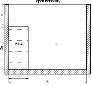
Description of the dam break problem. The geometry of the solution domain is shown in Fig. 1. The dimensions of the reservoir and the water column correspond to those used in the experiment carried out by Koshizuka et. al. [2]. The reservoir is made of glass, with a

base length of 0.584m. The water column, with a base length of 0.146m and the height of 0.292m (a=0.146m), was initially supported on the right by a vertical plate drawn up rapidly

at time t=0.0s. The water falls by gravity (g=9.81m/s2), acting vertically downwards. The

density of water is ρA=1000 kg/m

3_{, while the dynamic viscosity coefficient is}

A

µ =0.01kg/(m s). The density of air is taken to be ρB=1kg/m

3_{, and the dynamic viscosity coefficient is}

B µ =0.0001kg/(m s). a 4a a 2 a open boundary air water

Fig. 1. Geometry of a dam break problem.

The slip boundary conditions (4) are applied to the bottom and sides of the reservoir. The stress boundary conditions (5) are prescribed on the upper open boundary. They may be changed to fixed pressure and zero normal gradients of the velocities. The computations are performed on the structured finite element meshes of different resolution – 120×90 and 240 180. The investigated time interval is × t= [0.0; 1.0] s. The size of time step is

=

t

∆ 0.001667 for the 120×90 finite element mesh. The number of time steps is equal to 600. The size of the time step for the 240×180 finite element mesh is ∆t=0.000667. The number of the time steps used is equal to 1500.

Breaking wave phenomena and validation of numerical results. The breaking wave phenomenon is simulated by the pseudo-concentration method and the developed interface sharpening technique. Gravity causes the water column on the left of the reservoir to seek the lowest possible level of potential energy. Thus, the column will collapse and eventually come to rest. The initial stages of the flow are dominated by inertia forces with viscous effects in-creasing as the water comes to rest. On such a large scale, the effect of surface tension forces is insignificant. The complexity of velocity fields, occurring at different stages of breaking wave phenomena, can be easily captured using simple structured meshes.

Fig. 2. Visualization of breaking wave phenomena. 1.00 1.25 1.50 1.75 2.00 2.25 2.50 2.75 3.00 3.25 3.50 3.75 4.00 0.0 0.3 0.6 0.9 1.2 1.5 1.8 2.1 2.4 2.7 3.0 3.3 t* z/ a E1 E2 small big

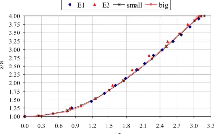
Fig. 3. Quantitative comparison of the numerical results and experimental measurements. Fig. 2 shows the screenshot of visualization e-service VizLitG illustrating the breaking wave phenomenon. Computed velocity field is represented by thresholded glyphs. Moving inter-face is captured by the iso-countour. Grey colours illustrate the pressure field while the chart plot shows variation of the pressure at the bottom. To predict the behaviour of the small bub-bles correctly is a more difficult task. When t=0.83 s, the backward moving wave has folded over and a small amount of air is trapped. However, in experiments, the air is present in the form of small bubbles. The current methodology has been derived for sharp interfaces; there-fore, the mesh needs significant refinement to a resolution smaller than the bubble size.

The numerical results have been validated by the quantitative comparison with experi-mental measurements obtained for the early stages of this experiment [1-2]. Non-dimensional position of the leading edge of the collapsing water column on the left wall versus non-dimensional time t* =t 2g/a is shown in Fig. 3. Two different sets of experimental data

E1 and E2 were presented by Martin and Moyce, illustrating the difficulty to determine the exact position of the leading edge. A thin layer of water shoots over the bottom and the rest of the bulk flow follow behind it. The accurate numerical results have been obtained by ap-plying intensive sharpening of the moving interface (ns=1, a=2.0). Almost identical values

have been obtained by using two structured finite element meshes of different resolution, 120×90 and 240×180 (the curve “small” and the curve “big”, respectively). The numerical

experiments have shown that the extreme sharpening is necessary only at the beginning of the time interval t=[0; 0.09] s. Thus, the accuracy of the obtained results is strongly influenced by the numerical parameters, but it is almost independent of the resolution of the finite ele-ment mesh, if sufficiently dense FE meshes are used.

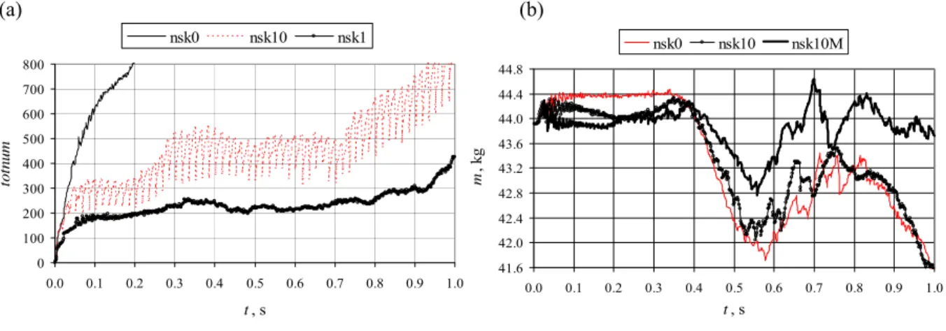
Interface sharpness and mass conservation. The quantitative comparison of the nu-merical results and the experimental measurements has shown that the detailed analysis of the interface sharpening parameters should be performed in order to develop an accurate and ef-ficient interface sharpening procedure. The sharpening frequency determines how often the interface sharpening procedure should be applied. Usually, interface sharpening has been performed at regular time intervals (each time step). Fig. 4a shows time evolution of the total number of nodes totnum, belonging to the interface (

ns

k

1

0<ϕ< ). The value of parameter

is fixed and equals to 1.5. The curve nsk0 illustrates how the interface grows without sharpening. It is obvious that this process is drastically influenced by the numerical diffusion. On the contrary, the interface sharpening performed at each time step reduces the interface thickness to one finite element (the curve nsk1). However, in this case, the moving interface can lose its smoothness. The results obtained in sharpening the interface less frequently are quite acceptable. The curve nsk10 visualizes the case =10.

a ns (a) (b) 0 100 200 300 400 500 600 700 800 0.0 0.1 0.2 0.3 0.4 0.5 0.6 0.7 0.8 0.9 1.0 t, s to tn u m nsk0 nsk10 nsk1 41.6 42.0 42.4 42.8 43.2 43.6 44.0 44.4 44.8 0.0 0.1 0.2 0.3 0.4 0.5 0.6 0.7 0.8 0.9 1. t, s m , k g 0 nsk0 nsk10 nsk10M

Fig. 4. Interface sharpness (a) and mass conservation (b).

Mass conservation is one of the most important tasks for any interface sharpening proce-dure. Fig. 4b shows mass evolution in time for several interface sharpening cases. The time interval t=[0.4; 0.7] s illustrates the case when water is leaving the computational domain and is coming back. In order to preserve the consistency between the flow physics and the numerical techniques, mass correction is automatically switched off in this special case. All plotted curves are actually of the same character, but quantitative results are quite different. The significant mass loss is observed when interface sharpening is not applied (the curve nsk0). The interface sharpening without mass correction at regular time intervals (the curve nsk10, 10) does not significantly reduce the mass loss. The application of mass correc-tion to regular interface sharpening (the curve nsk10M,

=

ns

=

ns 10) significantly improves mass

conservation. 6. Conclusions

In this paper, the dam break problem has been solved by the pseudo-concentration method and the developed interface sharpening technique. Dam break flow simulation has been effi-ciently performed on gLite based BalticGrid infrastructure. The numerical approach has been validated by quantitative comparison with the experimental measurements. The computed position of the leading edge of the collapsing water column has been in good agreement with the experimental data. The regular interface sharpening with mass correction is able to

pre-serve interface sharpness and mass conservation. The accurate numerical solution of the dam break problem, including highly non-linear breaking waves, proves that the developed nu-merical technique is capable of simulating moving interfaces undergoing large topological changes.

Acknowledgments

The work described in this paper is supported by the European Union through the FP7- INFRA-2007-1.2.3: e-Science Grid infrastructures contract No 223807 project "Baltic Grid Second Phase (BalticGrid-II)"

References

[1] J.C. Martin, W.J. Moyce // Philos. Trans. Roy. Soc. London, A244 (1952) 312.

[2] S. Koshizuka, H. Tamako, Y. Oka // J. Comput. Fluid Dynamics4 (1995) 29.

[3] F.H. Harlow, J.E. Welch // J. Phys. Fluids, 8 (1965) 2182.

[4] C.W. Hirt, B.D. Nichols // J. Comput. Physics39 (1981) 201.

[5] A. Masud, T.J.R. Hughes // Comput. Methods Appl. Mech. Eng.146 (1997) 91.

[6] F. Del Pin, E. Oñate, R. Aubry // Computers & Fluids36 (2007) 27.

[7] S. Osher, J.A. Sethian // J. Comput. Physics 79 (1988) 12.

[8] R. Löhner, C. Yang, E. Oñate // Comput. Methods Appl. Mech. Eng.195 (2006) 5597.

[9] E. Thompson // Int. J. Numer. Methods Fluids7 (1986) 749.

[10] R.W. Lewis, K. Ravindran // Int. J. Methods Eng. 47 (2000) 29.

[11] T.E. Tezduyar // Computers & Fluids,36 (2007) 207.

[12] D.A. Di Pietro, S. Lo Forte and N. Parolini //Appl. Numer. Math. 56 (2006) 1179.

[13] A. Kačeniauskas and P. Rutschmann // Int. J. Informatica, 15 (2004) 363.

[14] A. Kačeniauskas // Mechanika, 69 (2008) 35. [15] int.eu.grid: http://www.interactive-grid.eu/ [16] GlassFish: https://glassfish.dev.java.net/ [17] HDF5: http://hdf.ncsa.uiuc.edu/products/hdf5/

[18] VTK User's Guide Version 5, Inc. Kitware. 5th Edition, 2006.