The phase transitions of the planar random-cluster and Potts
models with
q
≥
1
are sharp
Hugo Duminil-Copin and Ioan Manolescu August 28, 2014
Abstract
We prove that random-cluster models with q≥1 on a variety of planar lattices have a sharp phase transition, that is that there exists some parameterpc below which the model
exhibits exponential decay and above which there exists a.s. an infinite cluster. The result may be extended to the Potts model via the Edwards-Sokal coupling.
Our method is based on sharp threshold techniques and certain symmetries of the lattice; in particular it makes no use of self-duality. Part of the argument is not restricted to planar models and may be of some interest for the understanding of random-cluster and Potts models in higher dimensions.
Due to its nature, this strategy could be useful in studying other planar models satisfying the FKG lattice condition and some additional differential inequalities.
1
Introduction
Main statement. The random-cluster model (or FK percolation) was introduced by Fortuin
and Kasteleyn in 1969 as a class of models satisfying specific series and parallel laws. It is related to many other models, including the q-state Potts models (q =2 being the particular case of
the Ising model). In addition to this, the random-cluster model exhibits a variety of interesting features, many of which are still not fully understood.
Consider a finite graph G = (VG, EG). The random-cluster measure with edge-weight p ∈ [0,1]and cluster-weight q>0on Gis a measureφp,q,G on configurationsω∈ {0,1}EG. An edge
is said to beopen (in ω) ifω(e) =1, otherwise it is closed. The configuration ω can be seen as
a subgraph of G with vertex set VG and edge-set {e∈EG∶ω(e) =1}. A cluster is a connected
component of ω. Let o(ω), c(ω) and k(ω) denote the number of open edges, closed edges and
clusters inω respectively. The probability of a configuration is then equal to φp,q,G(ω) = p
o(ω)
(1−p)c(ω)qk(ω) Z(p, q, G)
,
whereZ(p, q, G)is a normalizing constant called the partition function.
Consider a connected planar locally-finite doubly periodic graph G, i.e. a graph which is invariant under the action of some lattice Λ ≃ Z⊕Z. The model can be extended to G by
taking limits of measures on finite graphs Gn tending toG (with certain boundary conditions,
see Section 2.2 for details). We call such limitsinfinite-volume measures. As discussed later, for any pair of parametersp∈ [0,1] and q≥1, at least one infinite-volume measure exists, but it is
not necessarily unique. Forq≥1, the infinite-volume model exhibits a phase transition at some
critical parameter pc(q) (depending on the lattice). The aim of the present paper is to give a
proof of the sharpness of this phase transition.
Theorem 1.1. Fix q ≥ 1. Let G be a planar locally-finite doubly periodic connected graph
invariant under reflection with respect to the line {(0, y), y ∈ R} and rotation by some angle θ∈ (0, π) around0. There exists pc=pc(G) ∈ [0,1] such that
• for p<pc, there existsc=c(p,G) >0 such that for any x, y∈G,
φp,q[x and y are connected by a path of open edges] ≤exp(−c∣x−y∣), (1.1)
• for p>pc, there exists a.s. an infinite open cluster under φp,q,
where φp,q is the unique infinite-volume random-cluster measure on G with edge-weight p and
cluster-weight q.
Remark 1.2. The fact that, for p ≠ pc, there exists a unique infinite-volume measure with
edge-weight p may easily be shown by adapting [14, Thm. 6.17].
The sharpness of the phase transition was proved in arbitrary dimension for percolation in [1, 17] and for the Ising model in [2]. For planar random-cluster models with arbitrary cluster-weightq≥1, the sharpness had been previously derived only in the case of the square, triangular
and hexagonal lattices, see [3]. A similar result is proved for so-called isoradial graphs in [9]. It may be worth mentioning that, contrary to the present work, [3] and [9] are both based on integrability properties of the model.
The exponential decay of the two-point function is key to the study of the subcritical phase. It implies properties such as exponential decay of the cluster-size, finite susceptibility, Ornstein-Zernike estimates and mixing properties, to mention but a few. We do not go into details here, but rather refer the reader to the monographs [13, 14] for further reading.
Our method is based on the sharp threshold property and on certain symmetries of the lattice. A corollary of our results is that self-dual models are critical.
Corollary 1.3. The critical parameters pc(q) of the square, triangular and hexagonal lattices
satisfy
on the square lattice: pc(q) = √
q/(1+ √
q),
on the triangular lattice: pc(q) is the unique solution p in [0,1] of p3+3p2(1−p) =q(1−p)3,
on the hexagonal lattice: pc(q) is the unique solution p in [0,1] of p3−3qp(1−p)2=q2(1−p)3.
The model on the square lattice with the above parameter is indeed self-dual; the ones on the triangular and hexagonal lattices are not per se. They are dual to each other, but also related through the star–triangle transformation (see [14, Sec. 6.6]).
As mentioned above, the previous corollary was obtained in [3]. Nevertheless, the present method has the advantage of using self-duality for the identification of the critical point only, and not for the proof of sharpness (in [3], the self-duality is used in the proof of a Russo-Seymour-Welsh type estimate leading to the sharpness of the phase transition).
Extensions of Theorem 1.1 We discuss several (potential) generalisations of the previous
theorem.
First, the biperiodic graph G = (VG, EG) may be replaced by a weighted biperiodic graph (G, J), whereJ is a family of strictly positive weights on edges. For any subgraphG= (VG, EG)
of G andβ ≥0, we define φβ,q,G,J(ω) = ( ∏e∈EG(e βJe−1)ω(e) ) ⋅qk(ω) Z(β, q, G, J) , (1.2)
where Z(β, q, G, J) is a normalizing constant. One may easily see that in the case of Je = J
for any e∈EG, we obtain the previous definition with p=1−e−J β. As before, infinite-volume
measures may be defined on G by taking limits.
Theorem 1.4. Fix q ≥1. Let G be a planar locally-finite doubly periodic connected weighted
graph invariant under reflection with respect to the line {(0, y), y ∈ R} and rotation by some
• for β<βc, there exists c=c(β,G, J) >0 such that for any x, y∈G,
φβ,q,J[x andy are connected by a path of open edges] ≤exp(−c∣x−y∣),
• for β>βc, there exists a.s. an infinite open cluster under φβ,q,J,
where φβ,q,J is the unique infinite-volume random-cluster measure onG with parameters q and
β.
The proof of this theorem follows exactly the same lines as the one of Theorem 1.1 except that the notation becomes heavier. Thus we will only focus on Theorem 1.1.
A second potential extension is to planar random-cluster models with finite range interac-tions. Consider a planar graph G = (VG, EG) with the properties of Theorem 1.1. For some R≥1 define a modified graphG˜= (VG, EG˜), with same vertex set as G but with (u, v) ∈EG˜if
the graph distance betweenu and v inG is less than or equal toR. (ForR=1,G˜=G.)
We believe that our methods may be modified to prove Theorem 1.1 (and its inhomogeneous version Theorem 1.4) for G˜. In particular we expect that Theorem 1.1 also applies to the
random-cluster model on slabs, i.e. on the graphs of the formG × {0, . . . , R}d withd, R≥1. We
discuss this further in a forthcoming article.
A final potential extension is to models other than the random-cluster model. Our arguments are somewhat generic, and one can try to use them for models similar to those studied here. More precisely, to obtain our result, we only need the model to satisfy the conditions listed in Section 6. We discuss this point further in Section 6, when the appropriate notation is in place.
Consequences for the Potts model. Fix some finite weighted graph (G, J), where J = (Je)e∈E
G is a family of positive real numbers. Also fix a set of parametersβ≥0 and q∈Nwith
q≥2. The Potts model on Gwith q states and inverse temperatureβ is a probability measure µβ,q,G,J on {1, . . . , q}VG, for which the weight of a configurationσ is given by
µβ,q,G,J(σ) = e −βHq,G,J(σ) ZPotts β,q,G,J , where Hq,G,J(σ) = − ∑ e=(x,y)∈EG Je1σx=σy and ZPotts
β,q,G,J is a normalizing constant. The sum in the second equation is taken over all
un-ordered pairs of neighbours x, y.
A well-known coupling (sometimes called the Edwards-Sokal coupling) links the Potts and random-cluster models. We only briefly describe how to obtain the former from the latter. For details see [14, Thm 4.91].
Choose a random-cluster configuration ω according to φβ,q,G,J, where φβ,q,G,J is defined
as in (1.2). Assign to each cluster of ω a state (or colour) chosen uniformly in {1, . . . , q},
independently for different clusters. This generates a random configuration σ ∈ {1, . . . , q}VG.
(Note the two sources of randomness used in generating σ: the randomness in the choice of ω
and that in the colouring of the clusters ofω.) Then σ follows the Potts measureµβ,q,G,J.
Consider now a planar locally-finite doubly periodic weighted graph (G, J). As for the
random-cluster, infinite-volume Potts measures may be defined. The phase transition in this case is decided by the existence of long-range correlations. In particular, if βc is the critical
parameter, then
• forβ<βc, there exists a unique infinite-volume measure (long-range correlations vanish),
It follows trivially from the above coupling that
µβ,q,G,J(σx=σy) = 1 q +
q−1
q φβ,q,G,J(xand y are connected by a path of open edges),
hence the phase transition of the Potts model can be linked to that of the associated random-cluster model. In particular, when Je=J for all e∈EG,βc(q) = −J1 log(1−pc(q)).
Our main result may be translated as follows.
Theorem 1.5. Fix q ≥2. Let G be a planar locally-finite doubly periodic connected weighted
graph invariant under reflection with respect to the line {(0, y), y ∈ R} and rotation by some
angleθ∈ (0, π) around 0. There existsβc=βc(G, J) ≥0 such that,
• for β <βc, there exists a unique infinite-volume Potts measure µβ,q,J with parameters β
andq on (G, J). Moreover there exists c=c(β,G) >0 such that for any x, y∈G,
µβ,q,J[σx=σy] − 1
q ≤exp(−c∣x−y∣),
• for β > βc, there exist multiple infinite-volume Potts measures with parameters β and q
on (G, J).
Strategy of the proof. Let φ0
p,q be the infinite-volume measure on G with free boundary
conditions (see the next section for a precise definition). It is obtained as the limit of random-cluster measuresφp,q,Gn on finite subgraphs Gn of G that tend increasingly toG. Define
pc∶=inf{p∈ (0,1) ∶ φ0p,q(x is connected by a path of open edges to infinity) >0}
˜ pc∶=sup{p∈ (0,1) ∶ lim n→∞ −1 nlog[φ 0
p,q(0and ∂Λn are connected by a path of open edges)] >0}.
Note that p˜c ≤ pc. We wish to prove that pc = p˜c (this is simply another way of stating the
main result), and we therefore focus on the inequality p˜c≥pc. The proof of the latter is based
on the study of probabilities of crossing rectangles. For the sake of simplicity, let us restrict our attention in this introduction to rectangles of width 2n and height n, i.e. translates of [0,2n] × [0, n]. A rectangle iscrossed horizontally (vertically)if it contains a path of open edges
going from its left side to its right side (respectively from the bottom side to the top side). The strategy follows three main steps:
Step 1. We first prove that for any p>p˜c, the probability of crossing vertically (i.e. in the “easy
direction”) a rectangle of size2n×nis bounded away from 0 uniformly in n.
We show this by proving that for any0<ε<p, if theφ0p,q-probability of crossing vertically a
rectangle of size2n×ndrops below a certain benchmark (even for a single value ofn), then
theφp−ε,q,G-probability that two points are connected by an open path decays exponentially
fast (see Proposition 3.1 for the precise statement). A similar (but stronger) statement was proved by Kesten for percolation [16]. He proved that, given a percolation measure, if the probability of crossing the rectangle vertically is too small, then exponential decay follows for that measure. The difference with our result is that, in the case of percolation, one does not need to alter the parameter of the measure (see Remark 1.6 for more details). We highlight the fact that this part of the proof is not specific to the planar case.
Step 2. Using the first step, we show that for anyp>p˜c, the probability of crossing horizontally
(i.e. in the “hard direction”) a rectangle of size 2n×n is bounded away from 0 uniformly
in n.
This step is the most difficult. It corresponds to proving a “Russo-Seymour-Welsh” (RSW) type result: if crossing probabilities in the easy direction are bounded away from 0, then it
is the same in the hard direction. Such results were first proved in the context of Bernoulli percolation on the square lattice [18, 19]. Similar statements have been recently obtained for the Ising model [8, 5] and the random-cluster models with cluster-weight1≤q≤4[11],
but only for the square lattice. These results usually represent the first step towards a deep understanding on the critical phase.
In the present paper we prove a weaker statement than these RSW results: we show that, if crossing probabilities in the easy direction are bounded away from 0 for some
edge-weight p, then it is the same in the hard direction for anyp′
>p. As in the first step, the
difference with previous results is that we need to increase the edge-weight to obtain the desired conclusion.
Step 3. We show that if p<p′<pc are such that theφ0p,q-probability of crossing horizontally a
rectangle of size 2n×n is bounded away from 0 uniformly in n, then the φ0p′,q-probability
of these events tends to 1 asn tends to ∞.
This step is based on an argument from [12] that combines an influence theorem and a coupling argument to obtain a sharp threshold inequality (see Corollary 5.2).
Observe that these steps combine together to give the proof of the theorem. Indeed suppose
˜
pc<pcand takep˜c<p0<p1<p2<pc. By steps 1 and 2, the probabilities underφ0p
0,q of crossing
in the hard direction rectangles of size 2n×n are bounded away from 0, uniformly in n. By
step 3these crossing probabilities tend to 1 underφ0
p1,q. As a consequence the probability of a
dual crossing in the easy direction of a 2nby nrectangle tends to0. But step 1also applies to
dual measures, hence, for the edge-weight p2, the two-point function of the dual model decays
exponentially fast. This implies via a classical argument that there exists an infinite-cluster in the primal model, and this is a contradiction.
Remark 1.6. The proofs of Steps 1 and 2 require varying the edge-weight p. Nevertheless, we
expect that this is not indispensable. Bernoulli percolation is an example for which the proofs of Steps 1 and 2 are valid without changing p, but the known proofs of this fact rely heavily
on independence. In order to tackle more general models (in particular those having long-range dependence), we employ the differential inequality (2.6) invoking the Hamming distance, which entails altering p. The related differential inequality (2.5) is used in Step 3. Exploiting them to
their full strength is the main novelty of this article.
Open questions. We end this introduction by mentioning three related open questions.
The first is to investigate to which other models the methods of this paper may be adapted. We discuss this in Section 6, where we identify specific conditions for such models.
The second is to obtain results similar to Theorem 1.1 for lattices in dimensions d>2. We
believe that some of the techniques presented in this article can be harnessed in more general dimensions (we think in particular of Step 1 and inequalities (2.5) and (2.6)). Nevertheless, the methods of Steps 2 and 3 are based on certain features of planarity, and we are currently unable to extend Theorem 1.1 to higher dimension.
Finally we mention a broader direction of research. Just as the method of [3], our article provides very little information on the critical phase of the random-cluster model. Recent results (for instance [11, 20, 6, 7]) have illustrated that it is possible extract knowledge of the critical phase of random-cluster models from the theory of discrete holomorphic observables. But this theory is often based on integrability properties of the model, properties which are not true for general random-cluster models on planar locally-finite doubly periodic graphs. Therefore, it is very challenging to understand how to extend our knowledge of the critical random-cluster model on the square lattice to more general settings. A first step towards this goal is to prove that the results of Steps 1 and 2 are valid without changing the edge-parameter.
Organisation of the paper. Section 2 is dedicated to defining the model and explaining the
properties needed in the proof of Theorem 1.1. The next sections follow the steps described above: in Sections 3 and 4 we prove two finite size criteria for exponential decay (corresponding to Steps 1 and 2) that we then use in Section 5 to prove our main theorem (this corresponds to Step 3). In Section 6 we investigate a possible extension of the result to more general models.
2
Notations and basic facts on the model
2.1 Graph definitions
The lattice G. Fix for the rest of the paper a locally-finite planar connected graph G = (VG, EG) embedded in the plane R2 (in such a way that edges are straight lines intersecting at
their end-points only) and assume there exist u and v ∈R2 non collinear, and θ ∈ (0, π) such
that the following maps are graphs automorphisms of the embedded graph G: • the translations by vectorsuand v,
• the rotation of angleθ around 0,
• the orthogonal reflection with respect to the vertical line{(0, y), y∈R}.
It may be seen that, sinceG is required to be locally finite, there are only two possible values for
θ, namely π3 and π2. The triangular lattice is an example corresponding to the first case, while
the square lattice corresponds to the second (obviously, other examples may be given in both cases). For simplicity, we will only treat the case θ= π
2 in the following; the results also hold
in the case θ= π
3, with some standard adjustments of the proofs. It may be shown that, if we
allow some rescaling, we may consider the lattice to be invariant by • the translations by(1,0) and(0,1),
• rotation by π
2 around the origin,
• the orthogonal symmetry with respect to the vertical line{(0, y), y∈R}.
In the rest of this article, the graphG will be referred to as the lattice. Two vertices xand y of VG are said to be neighbours if(x, y) ∈EG. We then writex∼y.
The graph G= (VG, EG)will always denote a finite subgraph of G, i.e. EG is a finite subset
of EG and VG is the set of end-points of EG. We denote by∂G the boundary of G, i.e.
∂G= {x∈VG∶ ∃y∉VG withx∼y}.
Fora<b andc<d, letR= [a, b] × [c, d] be the subgraph ofG induced by the vertices ofVG
in[a, b] × [c, d]. This type of graph will be called a rectangle. For n≥0, letΛn= [−n, n]2.
Dual lattice and dual graphs. LetG∗be the dual lattice ofG, obtained by placing a vertex
in each face ofG and joining two vertices ofG∗if the corresponding faces ofG are adjacent. Note
thatG∗ enjoys the same symmetries asG. Fore
∈EG, sete∗ for the edge of G∗ intersecting e.
For a finite graphG, defineG∗ to be the graph with edge-setE
G∗ ∶= {e∗, e∈EG}, and vertex-set VG∗ given by the end-points of edges in EG∗.
The space of configurations. LetG= (VG, EG) be a subgraph of G. We will always work
with elements ω of Ω= {0,1}EG, called configurations. Edges e with ω(e) =1 are called open
(in ω), while others areclosed (inω). As mentioned above, ω can be seen as a subgraph of G
whose vertex-set isVG and edge-set is{e∈EG∶ω(e) =1}.
A path on Gis a sequence of vertices u0, . . . , un∈VG with(ui, ui+1) ∈EG fori=0, . . . , n−1.
It is calledopenif(ui, ui+1)is open inωfor everyi. Two verticesaandbare said to beconnected
(inωonG), if there exists an open path connecting them. The event thataandbare connected
is denoted bya←ω,GÐ→b(or simplya←G→bor evena←→bwhen no confusion is possible). Two setsA
andB are connected (denotedA←→B) if there exists a pair of connected vertices(a, b) ∈A×B.
When G= [a, b] × [c, d] is a rectangle and A= {a} × [c, d] and B = {b} × [c, d] (respectively A = [a, b] × {c} and B = [a, b] × {d}), the event A
ω,G
←Ð→ B is also denoted Ch([a, b] × [c, d])
(respectivelyCv([a, b] × [c, d])) and if it occurs we say thatGis crossed horizontally (respectively
vertically). An open path from A to B is called a horizontal crossing (respectively vertical
crossing). When a= 0 and c =0, we simply write Ch(b, d) and Cv(b, d) for the events above.
Whenb−a>d−c, horizontal crossings are called crossings in the hard direction, while vertical
ones are crossings in the easy direction. The terms are exchanged whenb−a<d−c.
To each configurationω∈Ωis associated a dual configurationω∗ onG∗ defined byω∗(e∗) =
1−ω(e). A dual-path onG∗ is a sequence of vertices u0, . . . , un∈VG∗ with(ui, ui+1) ∈EG∗ for i=0, . . . , n−1. It is calleddual-open if ω∗(ui, ui+1) =1 for all i. Two dual-verticesu and v are
said to be dual-connected (written u ω ∗,G∗
←ÐÐ→v or simply u ∗
←→v when no confusion is possible) if
there is a dual-open path connecting them. A maximal set of connected dual-vertices is called a dual-cluster. The definitions of crossings extend to dual configurations in the obvious way.
2.2 Basic properties of the random-cluster model
For more details and proofs we direct the reader to [14] or [7].
Boundary conditions. LetG= (VG, EG) be a finite subgraph of G. A boundary condition ξ
is a partition of∂G. We denote byωξthe graph obtained from the configurationωby identifying
(or wiring) the vertices in ∂G that belong to the same element of the partition ξ. Boundary
conditions should be understood as encoding how vertices are connected outside G. The
prob-ability measure φξp,q,G of the random-cluster model on G with parameters p∈ [0,1], q ≥0 and
boundary condition ξ is defined onΩby
φξp,q,G(ω) ∶= p o(ω) (1−p)c(ω)qk(ω ξ ) Zξ(p, q, G) , (2.1)
whereZξ(p, q, G) is a normalizing constant referred to as the partition function. Above, o(ω),
c(ω) and k(ωξ) correspond to the number of open and closed edges of ω, and the number of
clusters ofωξ.
Two specific boundary conditions are particularly important. The free boundary condition, denoted0, correspond to the partition composed of singletons only (no wiring between boundary
vertices). The wired boundary condition, denoted 1, correspond to the partition {∂G} (all
vertices are wired together). In addition to these two, we will sometimes consider boundary conditions induced by a configurationξ outsideG: two vertices are wired together if there exists
a path between them in ξ. We will identifyξ with the induced boundary condition and simply
write φξp,q,G for the corresponding measure.
Domain Markov property. LetG⊂F be two finite subgraphs ofG. A configurationωonF
may be viewed as a configuration onGby taking its restrictionω∣Gto edges ofG. The restriction
of the configurationω to edges of F∖G induces boundary conditions onGas explained below.
The domain Markov property states that for any p, q, any boundary conditionξ onF and any ψ∈ {0,1}EF∖EG,
φξp,q,F(ω∣G= ⋅ ∣ω(e) =ψ(e), e∈EF∖EG) =φψ
ξ
p,q,G(⋅), (2.2)
whereψξ is the partition induced by the equivalence relation xRy if x and y are connected in
ψξ.
The domain Markov property implies the following finite-energy property. For any ε> 0,
the conditional probability for an edge to be open, knowing the states of all the other edges, is bounded away from 0 and 1 uniformly in p∈ [ε,1−ε] and in the state of other edges. This
property extends to finite sets of edges (with a constant which gets worse and worse as the cardinality of the set increases).
Stochastic ordering for q ≥1. For anyG, the set {0,1}EG has a natural partial order. An
eventAis increasing if for any ω≤ω′,ω∈Aimpliesω′∈A. The random-cluster model satisfies
the following properties:
1. (FKG inequality) Fix p∈ [0,1],q ≥1 and some boundary condition ξ. Let A and B two
increasing events, thenφξp,q,G(A∩B) ≥φp,q,Gξ (A)φξp,q,G(B).
2. (comparison between boundary conditions) Fixp∈ [0,1],q≥1and ξand ψtwo boundary
conditions. Assume that ξ≤ψ, meaning that the partitionψ is coarser thanξ (there are
more wirings in ψthan inξ), then for any increasing event A,φξp,q,G(A) ≤φψp,q,G(A).
3. (comparison between different edge parameters) Fix p1 ≤ p2, q ≥ 1 and some boundary
conditionξ. Then for any increasing event A,φξp
1,q,G(A) ≤φ
ξ
p2,q,G(A).
Infinite-volume measures for q≥1. We will consider measures on infinite-volume
configu-rations, i.e. on{0,1}EG. Recall that for any finite subgraphGofG, a configurationω∈ {0,1}EG
induces a boundary condition on G that we will exceptionally write in this paragraph χ(ω).
Under χ(ω), two vertices x, y ∈∂G are wired if and only if they are connected in ω on G ∖G.
An infinite-volume random-cluster measure onG with parameters pand q is a measure φp,q on
{0,1}EG with the property that, for all finite subgraphsG ofG,
φp,q(ω∣G= ⋅ ∣χ(ω) =ξ) =φξp,q,G(⋅), (2.3)
for all boundary conditions ξ for which the conditioning is not degenerate.
The properties of the previous paragraph extend to infinite-volume measures by (2.3). One may prove that for any pair of parameters(p, q), there exists at least one such measure.
When q≥1, one may for instance take the limit of measures with wired (resp. free) boundary
conditions onΛn. The measure obtained in the limit is called the infinite-volume measure with
wired (resp. free) boundary conditions and is denoted byφ1p,q (resp. φ0p,q).
In general there is no reason that, for a given pair of parameters (p, q), there is a unique
infinite-volume measure. Nevertheless, for q≥1, the setDq of values ofp for which there exist
at least two distinct infinite-volume measures is at most countable, see [14, Theorem (4.60)]. This property can be combined with the stochastic ordering between different edge-weights to show the existence of a critical point pc∈ [0,1] such that:
• for any infinite-volume measure withp<pc, there is almost surely no infinite cluster,
• for any infinite-volume measure withp>pc, there is almost surely an infinite cluster.
When the planar, locally finite, doubly-periodic graph is non-degenerate, pc can be proved to
be different from 0 and 1 using a variant of the classical Peierls argument.
While the above is true also for lattices in higher dimensions, for planar lattices such as G
an additional argument shows thatDq⊆ {pc} (in fact in any dimension one hasDq⊆ [pc,1], see
[14, Theorem 5.16]). See the discussion following Remark 2.1 for details.
Planar duality. Let G be a finite graph and ξ ∈ {0,1}EG∖EG. If ω is distributed according
to φξp,q,G, the configurationω∗ is also distributed as a random-cluster configuration onG∗ with
different parameters. More precisely, we find that
φξp,q,G(ω) =φξp∗∗,q∗,G∗(ω ∗ ), where pp∗ (1−p)(1−p∗) =q and q∗=q
andξ∗ is the boundary condition on ∂G∗ induced by the dual-configurationξ∗
∈ {0,1}EG∗∖EG∗.
For instance, dual measures extend to the whole of G∗ and, if ω follows φ1
p,q,G (respectively φ0 p,q,G), then ω ∗ is distributed asφ0 p∗,q,G∗ (respectivelyφ 1 p∗,q,G∗).
Remark 2.1. As a consequence of Theorem 1.1, forq≥1 andp>pc, there exists c=c(p, q) >0
such that
φp,q(u ∗
←→v) ≤exp(−c∣u−v∣), for all u, v∈VG∗. (2.4)
Indeed, an adaptation of Zhang’s argument (as that of [14, Thm 6.17]) shows that, for any values of q≥1 and p∉Dq, it is impossible to have with positive probability infinite clusters in
both ω and ω∗. Thus, if
p>pc, there is no infinite cluster in ω∗, and Theorem 1.1 applied to
the dual random-cluster model implies (2.4).
Differential inequalities. The two following theorems are essential to our study. The first is
a direct adaptation of the more general statement of Graham and Grimmett [12, Thm. 5.3].
Theorem 2.2 ([12]). For any q ≥1 there exists a constant c>0 such that, for any p∈ (0,1),
any finite graph G, any boundary condition ξ and any increasing event A, d dpφ ξ p,q,G(A) ≥c φ ξ p,q,G(A)(1−φ ξ p,q,G(A))log( 1 2mA,p ), (2.5)
where mA,p=maxe∈EG(φ
ξ
p,q,G(A∣ω(e) =1) −φ ξ
p,q,G(A∣ω(e) =0)).
The original result concerns a more general class of measures than that of the random-cluster model, hence the slightly more complicated statement of [12, Thm. 5.3]. The above formulation is easily deduced using an explicit bound for the finite energy property of the random-cluster model:
p q ≤φ
ξ
p,q,G(ω(e) =1∣ω(f), f ≠e) ≤p, for all G, e, ξ, pandq≥1.
In order to state the second result, we introduce the notion of Hamming distance. For an eventA and a configuration ω, define HA(ω) as the graph distance in the hypercube {0,1}EG
(or Hamming distance) between ω and the setA. When A is increasing, it corresponds to the
minimal number of edges that need to be turned to open in order to go from ω to A. The
following may be found in [14, Thm. 2.53] or [15].
Theorem 2.3 ([15]). For any q≥1, any p∈ (0,1), any finite graph G and boundary condition ξ, we have that for any increasing event A,
d dplog(φ ξ p,q,G(A)) ≥ φξp,q,G(HA) p(1−p) . (2.6)
In the above φξp,q,G(HA) is the expectation ofHA underφξ
p,q,G.
Remark 2.4. In this article (2.6) will be used in its integrated form. Consider two valuesp′ <p
and an increasing event A. Since HA is a decreasing function, by integrating (2.6) between p′
and p we find φξp′,q,G(A) ≤φ ξ p,q,G(A)exp[ −4(p−p ′ )φξp,q,G(HA)]. (2.7)
Now, consider an event A depending on a finite set of edges E and assume that the
infinite-volume measures atp′ andpare unique. By takingξ
=1and taking the limit in (2.7) asGtends
to G (both sides of the inequality converge) we obtain
From now on, we fix q≥1 and G. For ease, we drop them from the notation. We
will frequently work with infinite-volume measures for different values of p and will always assume that these values are not in Dq. In such case, φp means the unique
infinite-volume measure with parameter p.
Remark 2.5. Since Dq is countable, the different claims could be easily extended to values of p
in Dq by density (φp simply denotes any infinite-volume measure in this case). Also note that
we are mainly interested in p<pc for which p∉Dq anyway (we prefer to state the claims in full
generality since they may be of some use in other contexts).
3
Crossings in the easy direction
The goal of this section is to prove the following result, which corresponds to Step 1.
Proposition 3.1. If p0∈ (0,1) is such that there exists an infinite-volume measureφp0 with
lim inf n→∞
φp0(Cv(2n, n)) =0,
then for any p<p0 there existsc=c(p) >0 such that for any x, y∈G φp(x←→y) ≤exp(−c∣x−y∣).
Remark 3.2. This proposition can be proved in any dimension d ≥ 2. The claim should be
adapted as follows: if the liminf of probabilities of crossing sets of the form [0,2n]d−1× [0, n]
from [0,2n]d−1 × {0} to [0,2n]d−1 × {n} is equal to 0 for some edge-weight p0, then there is
exponential decay for any p<p0 (i.e. (1.1) holds for p<p0).
The proof of the proposition is based on the following two lemmas. Let Cx be the cluster of
the sitex. For simplicity we will henceforth assume0∈VG.
Lemma 3.3. Let p0 > 0. If there exists an infinite-volume measure φp0 and κ > 0 such that φp0(∣C0∣
4+κ) < ∞, then for any p<p
0, there existsc=c(p) >0 such that for any n≥0,
φp(0←→∂Λn) ≤exp(−cn). (3.1)
It is easy to see that (3.1) is equivalent to exponential decay, as defined in (1.1). The previous lemma is classical, see [15] or [14, Thm. 5.64]. We only mention that its proof is based on the differential inequality (2.6).
Lemma 3.4. Let p>p′. For any N ≥n,
φp′(Cv(2N, N)) ≤exp[−(p−p′)N
n(1−φp(Cv(2n, n)))
2N/n ].
Proof Consider the eventCv(2N, n). Any vertical open crossing of[0,2N] × [0, n]contains at
least one of the following:
• a vertical crossing of a rectangle[kn,(k+2)n] × [0, n], for some 0≤k< ⌊N/n⌋,
• a horizontal crossing of a square[kn,(k+1)n] × [0, n], for some 0≤k< ⌊N/n⌋.
All the events above have probability bounded from below by φp(Cv(2n, n)). Using the FKG
inequality for the complements of these events, we obtain
1−φp(Cv(2N, n)) ≥ (1−φp(Cv(2n, n))) 2N/n
. (3.2)
As a consequence, we deduce that
φp(HC
v(2N,n)) ≥φp(HCv(2N,n)≥1) =1−φp(Cv(2N, n)) ≥ (1−φp(Cv(2n, n))) 2N/n
SinceCv(2N, N) is included in the intersection of⌊N
n⌋ translates of Cv(2N, n), it follows that
φp(HC v(2N,N)) ≥ ⌊ N n⌋(1−φp(Cv(2n, n))) 2N/n . By (2.8) for p′
< p we find the result (we have ignored the integer parts in the lemma since 1
p(1−p)⌊N/n⌋ ≥N/n). ◻
The idea of the proof of Proposition 3.1 goes as follows. Assuming thatφp(Cv(2n, n))is small
for somen, we apply Lemma 3.4 repeatedly, and obtain a bound on the decay ofφp−ε(Cv(2N, N))
asN increases. A bound on the moments of ∣C0∣follows.
Proof of Proposition 3.1 Fix some ε> 0 and p0 > ε. Let α > 2 be a (large) constant, we
will see later how to choose it. (We prefer not to give an explicit value for α now, though the
requirements for it are universal.) Consider a small constantδ0>0, we will see in the proof how
to chooseδ0 (its value only depends on αandε). Assume that there exists a positive integern0
such thatφp0(Cv(2n0, n0)) ≤δ
α
0 and define recursively, fork≥0, δk+1=δk2,
nk+1=nk/δk2, pk+1=pk−δk.
Assuming δ0 is sufficiently small, the inequalityφpk(Cv(2nk, nk)) ≤δ
α
k and Lemma 3.4 imply
φpk+1(Cv(2nk+1, nk+1)) ≤exp(−(pk−pk+1) nk+1 nk (1−φpk(Cv(2nk, nk)))2nk+1 /nk ) ≤exp( − (1−δαk)2δ −2 k δk ) ≤δk2α=δαk+1.
Further assume thatδ0 is chosen small enough thatlimk→∞pk≥p0−ε. We deduce that for any k≥0,
φp0−ε(Cv(2nk, nk)) ≤δ
α
k. (3.3)
Let us extend the previous bound to values of N different from the {nk∶k≥0}. For nk≤N < nk+1, by (3.2) or by a simple union bound,
φp0−ε(Cv(2N, N)) ≤φp0−ε(Cv(2N, nk)) ≤ 2nk+1 nk δkα≤2( n0 N) α−2 4 .
In the last inequality we have used that δi=δ1/2
k−i
k for any i≤k, and therefore
δ4k≤ k ∏ i=0 δ2i = n0 nk+1 ≤n0 N.
It easily follows that φp0−ε(0↔∂ΛN) ≤8(
n0
N)
α−2
4 for any N. Since a cluster of cardinality
larger than N has diameter at least a constant times √N, we find easily that φp−ε(∣C0∣ 5) < ∞
provided thatα is chosen large enough (α>42 suffices). By Lemma 3.3, the above implies that
for any p<p0−ε, there exists c=c(p) >0 such that for any n≥0, φp(0←→∂Λn) ≤exp(−cn).
Now, iflim infφp0(Cv(2n, n)) =0,then for anyε>0, there existsn0such thatφp0(Cv(2n0, n0)) ≤
δα
0, whereαandδ0=δ0(ε, α)are chosen as above. By the argument aboveφpexhibits exponential
4
Crossing probabilities in the hard direction
The object of this section is the following result.
Proposition 4.1. If p∈ (0,1) is such that there exists an infinite-volume measureφp with
lim inf n→∞
φp(Cv(2n, n)) >0, (4.1)
then for any p0 >p,
lim inf n→∞
φp0(Ch(2n, n)) >0.
In light of Proposition 3.1, the above result has the following immediate corollary, which is exactly the claim mentioned in Step 2 of the introduction.
Corollary 4.2. If p0∈ (0,1) is such that there exists an infinite-volume measure φp0 with
lim inf n→∞
φp0(Ch(2n, n)) =0, then for any p<p0 there existsc=c(p) >0 such that for any n≥0,
φp(0←→∂Λn) ≤e−cn.
The proof of Proposition 4.1 is based on the following lemma and its corollary. Some termi-nology is needed for their statement. Letγ1, . . . , γK be open paths in some rectangle[a, b]×[c, d].
We say they areseparated in[a, b] × [c, d]if they are contained in distinct clusters of[a, b] × [c, d]
(beware of the fact that we are speaking of clustersin[a, b] × [c, d]). In other words, no two are
connected by open paths inside[a, b] × [c, d].
Lemma 4.3. Let p ∈ (0,1) and n ∈N. There exist universal constants c0, c1 >0 such that, if
1≤I ≤n/400 is an integer that satisfies
I2≤c0
φp(Cv(2n, n))
φp(Ch(2n, n))c1/I, (4.2)
then
φp([0,2n] × [0, n/2] has 2I separated vertical crossings) ≥12φp(Cv(2n, n)). (4.3)
The statement above may seem cryptic. Here are a few observations that may help the reader assimilate the lemma. First of all, the conclusion (4.3) is strongest when I is large, but
the hypothesis (4.2) is effectively an upper bound on I. Moreover it may even be that there
exists no I with the properties required in the lemma. The lemma will be applied in situations
whereφp(Cv(2n, n))is bounded below by some constant. Then it states that, ifφp(Ch(2n, n))is
close to0(so thatImay be large and satisfy (4.2)), the rectangle[0,2n] × [0, n/2]contains many
separated vertical crossings with positive probability. Furthermore, the smaller φp(Ch(2n, n)),
the larger the number of separated vertical crossings.
In words, this statement asserts that if typically [0,2n] × [0, n] is crossed vertically, but the
probability of crossings in the hard direction is very small, then any vertical crossing needs to twist substantially, creating many separated crossings of a slightly smaller (in height) rectangle (see the discussion preceding the proof of Lemma 4.3).
The proof of Lemma 4.3 represents the major difficulty of this article. We postpone it to the end of the section and first explain how it implies Proposition 4.1. A key observation is that the existence of separated vertical crossings of[0,2n] × [0, n/2](as in (4.3)) implies a lower bound on
the Hamming distance to the event Ch(2n, n). Using (2.6), this yields an explicit lower bound
For x∈ (0,1), set f(x) ∶= ⎧ ⎪ ⎪ ⎨ ⎪ ⎪ ⎩ log(1/x) log log(1/x) if x<1/e −∞ otherwise .
Corollary 4.4. Let δ>0. There exist constants c2=c2(δ) >0 and c3 =c3(δ) >0 such that for
any p>p′ and nwith φp(Cv(2n, n)) ≥δ andn≥c2f[φp(Ch(2n, n))], the following holds:
φp′(Ch(n, n/2)) ≤exp[ −c3(p−p′)δexp(c3f[φp(Ch(2n, n))])].
Proof Fix δ > 0 and p > p′. Let n be an integer such that φp(Cv(2n, n)) ≥ δ and n ≥ c2f[φp(Ch(2n, n))], for a constant c2 specified later. Define I = ⌊cff[φp(Ch(2n, n))]⌋, where cf =cf(δ)is some large constant to be specified. It is easy then to see that, for this choice of I,
we have
I2≤c0
φp(Cv(2n, n)) φp(Ch(2n, n))c1/I
for every n ≥ 1, provided that cf is large enough (where c0, c1 are the universal constants of
Lemma 4.3). Furthermore, we find that I ≤n/400by setting c2 =400cf. Finally, we may limit
ourselves to the case where φp(Ch(2n, n))is small enough to have I ≥1 (the constant c3 may
be chosen so that the conclusion holds trivially otherwise).
The previous paragraph shows that with these choices ofcf andc2,Isatisfies the assumptions
of Lemma 4.3, and we find
φp([0,2n] × [0, n/2]contains 2I separated vertical crossings) ≥ 1
2φp(Cv(2n, n)) ≥
δ
2.
Since the crossings in (4.3) are separated, there exist also at least 2I−1 ≥ 2I−1 disjoint dual
vertical crossings of [0,2n] × [0, n/2]. This generates a lower bound on the expected Hamming
distance to the eventCh(2n, n/2):
φp(HC
h(2n,n/2)) ≥2
I
⋅δ
4. (4.4)
Inequality (2.8) (the integrated form of (2.6)) implies that
φp′(Ch(2n, n/2)) ≤φp(Ch(2n, n/2))exp( −
1
p(1−p)
⋅ (p−p′) ⋅2I⋅δ4)
≤exp[ − (p−p′)δexp(c3f[φp(Ch(2n, n))])],
where the constantc3>0 depends oncf and therefore onδ only. In the last inequality, we used
the choice of I proposed at the very beginning of the proof. Finally, by combining crossings in
the hard direction of five rectangles with side lengths n and n/2, we may obtain a crossing of
[0,2n] × [0, n/2]. Thus,
φp′(Ch(n, n/2)) 5
≤φp′(Ch(2n, n/2)),
and the result follows. ◻
Proof of Proposition 4.1 Fix p0 >p and assume that inf
n≥0φp
(Cv(2n, n)) =δ > 0. Let c2, c3
be the constants given by Corollary 4.4 forδ given above. For integers n0 and 0≤k≤log2 √ n0, define nk=2−kn0, pk=p0− (p0−p) k ∑ i=1 2−i , βk=φp k(Ch(2nk, nk)).
We aim to apply Corollary 4.4 with the above values ofnandp. We start by a simple verification
of the hypothesis.
Claim. Forn0 large enough and for any integer 0≤k≤log2 √
n0, nk>c2f(βk).
Proof of the Claim. Assume that there exists an integer0≤k≤log2 √ n0such thatnk≤c2f(βk). We have φp(Ch(2nk, nk)) ≤φp k(Ch(2nk, nk)) =βk≤exp( − nk c2 ) ≤n−10k , (4.5)
where the second inequality uses thatf(x) ≤log(1/x). In the last inequality we have supposed
thatnk is larger than some rank depending only onc2. We may assume this sincenk≥ √
n0 and
we may taken0 as large as we wish.
Consider x∈ {0} × [0, nk] andy∈ {1
2nk} × [0, nk] maximizing (among such pairs of vertices)
the probability that they are connected in[0,1
2nk] × [0, nk]. Then φp(x [0,nk/2]×[0,nk] ←ÐÐÐÐÐÐÐ→y) ≥ 1 n2 k φp(Ch(1 2nk, nk)).
Combining four times the above (also using reflection symmetry) we obtain
φp(Ch(2nk, nk)) ≥
1
n8
k
φp(Ch(12nk, nk))4.
Confronting this to (4.5) implies
φp(Ch(12nk, nk)) ≤n−1/2k ≤n−1/40 .
But φp(Ch(12nk, nk)) ≥ δ by assumption and symmetry under π2-rotation. This leads to a
contradiction for n0 large enough.
The argument that (4.5) contradicts φp(Ch(1
2nk, nk)) ≥δ will be used several times in the
rest of the paper.
◇
We now fix n0 large, in particular large enough for the property of the claim to be satisfied.
Then we may apply Corollary 4.4 to each triplet (nk, pk, pk+1) to obtain βk+1≤exp( −c32−(k+1)(p0−p)δexp(c3f(βk))).
Hence, there exist constants ∆≥e40 and c∆>0, depending on p0−p, c3 and δ only, such that
if we assumeβk≤c∆∆−k, the previous displayed equation implies that
c3f(βk) ≥2klog 2 and βk+1≤exp[ −c3(p0−p)δexp(c3
2f(βk))] ≤
βk
∆ ≤c∆∆
−(k+1) .
Assume now that β0 ≤c∆. Then, by the above, βk ≤c∆∆−k for any k≤log2 √ n0. Therefore, there exists m∈ [ √ n0, n0] (m=n⌊log 2 √ n0⌋) such that φp(Ch(2m, m)) ≤c∆e−40⌊log2 √ n0⌋ ≤c∆m−10.
Using the same procedure as at the end of the proof of the previous claim we obtain a contra-diction forn0 large enough, since m≥
√
n0 and φp(Ch(2m, m)) ≥δ by definition.
Therefore, the assumptionφp0(Ch(2n0, n0)) =β0≤c∆can not hold forn0large enough. This
implies that
lim inf n→∞
φp0(Ch(2n, n)) ≥c∆>0.
◻
We now turn to the core of the argument, namely the proof of Lemma 4.3. The proof is inspired by the work of Bollobás and Riordan on Bernoulli percolation on Voronoi tessellations [4] (even though it makes use of different ingredients, and that the claim is not the same). We start with a brief description.
Fix I as in Lemma 4.3 and let v = 1
100I. First we obtain an upper bound, as a function
of φp(Ch(2n, n)), for the probability of crossing horizontally rectangles of height k and width (1+v)kfork∈ [n4, n]. Using this bound, we show that one vertical crossing of[0,2n] × [0, n]
con-tains, with high probability, three crossings of the slightly thinner rectangle[0,2n] × [23vn,(1−
23v)n]. Repeating the procedure, we finally obtain 2I crossings of[0,2n] × [n 4,
3n
4 ]. Moreover,
these crossings are separated by dual paths. See Figure 4.
Proof of Lemma 4.3 Fixp, nandI satisfying the assumptions of the lemma and setv= 1 100I
(we will specify the values of the universal constants c0 and c1 later in the proof). Define α=sup{φp(Ch(⌈(2+v)k⌉,2k)) ∶k∈ [n 8, n 2]}. (4.6) For any k ∈ [n 8, n
2], we may combine 32/v crossings in the hard direction of rectangles with
sides of length 2k and ⌈(2+v)k⌉ (both horizontal and vertical) to create a horizontal crossing
of [0,2n] × [0, n]. Choosing k∈ [n 8,
n
2] achieving the maximum in (4.6), we conclude that α≤φp(Ch(2n, n))v/32≤φp(Ch(2n, n))2c1/I, (4.7)
by settingc1=1/6400.
We start by proving a series of claims that will then be used to prove the lemma. For these claims, fix an integer k ∈ [n
4,
n
2] and u ∈ [v,1/3] such that ku ∈ Z. The first three claims are
concerned with crossings of the rectangleR(k) = [−(1+u)k,(1+u)k] × [0,2k].
Claim 1. Let E(k) be the event that there exists a vertical open crossing of R(k), with the
lower endpoint not contained in [−3uk,3uk] × {0}, or the higher endpoint not contained in [−3uk,3uk] × {2k}. Then
φp(E(k)) ≤4(α+ √
α).
Proof of Claim 1. Letβ be theφp-probability that there exists a vertical open crossing ofR(k),
with the lower endpoint in[−(1+u)k,−3uk] × {0}.
The probability of crossing[−(1+u)k,(1−2u)k] × [0,2k]vertically is at mostα(by definition
ofα). Thus, with probability β−α, there exists a vertical crossing of R(k)with an endpoint in [−(1+u)k,−3uk] × {0}which intersects the vertical line {(1−2u)k} × [0,2k]. See Figure 1. By
reflection with respect to {−3uk} × [0,2k], with probability β−α, there exists an open path in [−(1+4u)k,(1−5u)k] × [0,2k], between [−3uk,(1−5u)k] × {0} and {−(1+4u)k} × [0,2k].
When combining the two events above using the FKG inequality, we obtain that, with probability at least (β−α)2, there exists a horizontal open crossing of[−(1+4u)k,(1−2u)k] × [0,2k]. This event has probability less than α, hence β ≤ α+
√
α. By considering the other
(1−2u)k (2 + 2u)k (1−2u)k O 3uk 2k γ1 γ2 3uk
Figure 1: In the black rectangle R(k), a path γ1 connects [−(1+u)k,−3uk] × {0} to the top
side. Except on an event of probability α, γ1 crosses the vertical line {(1−2u)k} × [0,2k]
(grey). By reflection we may construct a pathγ2, contained in
[−(1+4u)k,(1−5u)k] × [0,2k],
and connecting[−3uk,(1−5u)k] × {0} and{−(1+4u)k} × [0,2k]. The two induce a horizontal
crossing of the grey rectangle [−(1+4u)k,(1−2u)k] × [0,2k].
◇
Claim 2. Let F(k) be the event that there exists a vertical open crossing of R(k) that does not
intersect the vertical line{(1−2u)k} × [0,2k]. Then φp(F(k)) ≤2α.
Proof of Claim 2. Any vertical crossing of R(k) not touching {(1−2u)k} × [0,2k] is either
contained in[−(1+u)k,(1−2u)k] × [0,2k]or[(1−2u)k,(1+u)k] × [0,2k]. Both these rectangles
are crossed vertically with probability less thanα, and the claim follows (we used that u≤1/3). ◇
Claim 3. Let G(k) be the event that there exists an open path in R× [0,(2−11u)k] between [−3uk,3uk] × {0} and the vertical segment {(1−2u)k} × [0,(2−11u)k]. Then
φp(G(k)) ≤α+ √
α.
Proof of Claim 3. Let β = φp(G(k)). Suppose G(k) occurs and let γ be an open path in
R× [0,(2−11u)k] between [−3uk,3uk] × {0} and {(1−2u)k} × [0,(2−11u)k]. There are two
possibilities forγ. Eitherγ crosses the line {−(1−8u)k} × [0,(2−11u)k], or it does not.
The first situation arises with probability at mostα, since it induces a horizontal crossing of
the rectangle [−(1−8u)k,(1−2u)k] × [0,(2−11u)k]. See the left diagram in Figure 2.
Thus the second situation arises with probability at least β−α. Then, by symmetry with
respect to{3uk} ×Rand the FKG inequality, with probability at least(β−α)2,[−(1−8u)k,(1−
2u)k] × [0,(2−11)k] contains two open paths:
• one connecting[−3uk,3uk] × {0} to {(1−2u)k} × [0,(2−11u)k],
• one connecting[3uk,9uk] × {0}to {−(1−8u)k} × [0,(2−11u)k].
These two paths induce an open horizontal crossing of[−(1−8u)k,(1−2u)k] × [0,(2−11u)k],
(1−2u)k (1−8u)k (2 − 11 u ) k 6uk
Figure 2: The two possibilities for the path γ. The black rectangleR(k) is depicted for scaling
purposes, and the stripR× [0,(2−11u)k]is delimited by the top grey line. The origin is marked
by a disk. Left: the first situation, the pathγcrosses the vertical line{−(1−8u)k}×[0,(2−11u)k].
Right: two occurrences of the second situation may be used to create a horizontal crossing of
[−(1−8u)k,(1−2u)k] × [0,(2−11u)k].
◇
In the claims above we have defined the events E(k),F(k) and G(k). In addition, define ̃
G(k) as the symmetric ofG(k) with respect to the lineR× {k}, i.e. the event that there exists
an open path in R× [11uk,2k] between [−3uk,3uk] × {2k} and {(1−2u)k} × [11uk,2k]. The
bound of Claim 3 applies toG̃(k)as well.
All four events revolve around the rectangleR(k). In the following, we will use translates of
these events, and we will say for instance that E(k) occurs in some rectangle R(k) +z if E(k)
occurs for the translate of the configuration by −z.
Claim 4. Except on an event H(k) of probability at most 1
u(54α+36
√
α), any open vertical
crossing of S(k) = [0,2n] × [−k, k], contains two separated vertical crossings of S((1−11u)k) = [0,2n] × [−(1−11u)k,(1−11u)k].
Proof of Claim 4. The rectangle [0,2n] × [−k, k] is the union of the rectangles Rj = [juk,(2+ (j+2)u)k] × [−k, k], for0≤j≤J, where
J ∶= ⌊1
u( n
k−2)⌋ −2 ≤ 6/u.
LetH(k) be the union of the following events for 0≤j≤J:
• the rectangle[juk,(2+ (j+1)u)k] × [−k, k] contains a horizontal open crossing,
• E(k) occurs in the rectangle Rj,
• F(k) occurs in the rectangle Rj,
• at least one ofG(k) and G˜(k)occurs in the rectangle Rj.
Using a simple union bound and the estimates of Claims 1-3, we obtain
φp(H(k)) ≤
100√α
u . (4.8)
Consider a configuration not in H(k) containing a vertical open crossing γ of S(k). We are
γ
1γ
2γt
γs
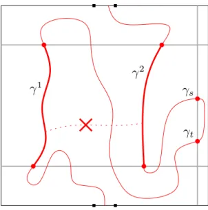
Figure 3: The path γ under the assumption thatE(k),F(k), G(k) andG˜(k) do not occur in Rj. The endpoints are contained in segments of length 6uk around the centres of the top and
bottom sides. A first crossing of the stripS((1−11u)k)occurs betweenγ0 andγt, and a second
between γs and γ1. The two crossings γ1, γ2 need to be separated to ensure that F(k), G(k)
and G˜(k)do not occur.
will not use this fact here) separated crossings ofS((1−11u)k). We recommend that the reader
takes a look at Figure 3 first.
Since none of the rectangles[juk,(2+(j+1)u)k]×[−k, k]is crossed horizontally,γis contained
in one of the rectangles Rj. Fix the corresponding index j. Parametrize γ by [0,1], with γ0
being the lower endpoint.
SinceE(k)does not occur inRj,γ0andγ1, are contained in[(1+ (j−2)u)k,(1+ (j+4)u)k] × {−k} and [(1+ (j−2)u)k,(1+ (j+4)u)k] × {k}, respectively. Moreover, since F(k) does not
occur in Rj, γ crosses the vertical line {(2+ (j−1)u)k} × [−k, k]. Let t and s be the first and
last times that γ intersects this vertical line.
Since G(k) does not occur in Rj,γ intersects the line [0,2n] × {(1−11u)k} before time t.
Likewise, since G˜(k) does not occur, γ intersects the line [0,2n] × {−(1−11u)k} after time s.
This implies that γ contains at least two disjoint crossings of S((1−11u)k). Call γ1 the first
one (in the order given by γ) and γ2 the last one.
The above holds for any vertical crossing γ of S(k), hence the crossings γ1 and γ2 are
necessarily separated inS((1−11u)k). Indeed, if they were connected insideS((1−11u)k), then
F(k) would occur.
◇
Remark 4.5. It is actually possible to prove that, in the situation described above, γ contains
at least three separated vertical crossings of S((1−11u)k). We do not detail this as it is not
essential for our proof, but the situation will be depicted in the relevant figures.
Getting back to the proof of the lemma. Let ki = ⌊(1−22vi)n/2⌋ for 0 ≤ i≤ I. We will
investigate vertical crossings of the nested strips S(ki) = [0,2n] × [−ki, ki]. Note that S(k0) is
contained in a translation of the rectangle[0,2n] × [0, n], and thatS(kI)contains a translation
of the rectangle[0,2n] × [0, n/2].
Fix a sequence (ui)i, with ui ∈ [v,2v] and kiui ∈Z for 0≤i<I. The existence ofui is due
to the fact that v ≥ 4
n (since I ≤n/400). Define the events H(ki) of Claim 4 for these values
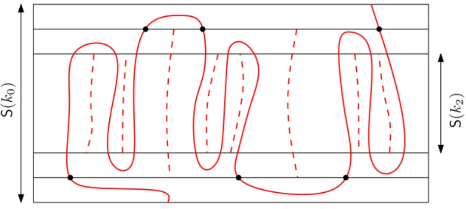
S ( k0 ) S ( k2 )
Figure 4: Under (∪Ii=0−1H(ki))c, one vertical crossing ofS(k0) contains two (in fact even three)
separated crossings of S(k1) (with marked endpoints). Each such crossing contains in turn
two (in fact even three) separated crossings of S(k2). This generates four (in fact even nine)
separated crossings inS(k2), and thus three (in fact even eight) dual crossings between them.
crossings of S(kI) which are separated in S(kI). Indeed, by Claim 4, every crossing of S(ki)
contains two separate crossings of S(ki+1) ⊂S((1−11ui)ki). See Figure 4. By the union bound
and Claim 4, φp( I−1 ⋃ i=0 H(ki)) ≤ 100 √ α u I ≤10 000 √ αI2≤ φp(Cv(2n, n)) 2 ,
where the second inequality is due to the choice ofI and the fact that we may assumec0≤ 1 20 000
(see (4.2) and (4.7)). But S(k0) is crossed vertically with probability at least φp(Cv(2n, n)).
Thus, with probability at leastφp(Cv(2n, n))/2,S(kI) contains 2I separated vertical crossings.
The claim follows from the fact thatS(kI) contains a translate of [2n, n/2]. ◻
5
Proof of Theorem 1.1
The following coupling argument may be used in conjunction with Theorem 2.2 of Graham and Grimmett to obtain sharp threshold results, as in [12, Lem. 6.3]. In our case the desired result is stated subsequently as a corollary. For an edgeeand a configuration ω, write Ce(ω) for the
open cluster ofeinω, i.e. for the union of the open clusters of the endpoints ofe.
Proposition 5.1. LetGbe a finite graph,e∈EGbe an edge and ξ be a boundary condition. For q≥1andp∈ (0,1) there exists a measure ΦonΩ×Ωsuch that, if (π, ω)is distributed according
to Φ,
• π is distributed according to φξp,q,G(.∣π(e) =0),
• ω is distributed according to φξp,q,G(.∣ω(e) =1),
• Φ-almost surelyπ≤ω andπ(f) =ω(f) for edges f ∉Ce(ω).
Corollary 5.2. For any0<p0<p1<1, there exists c=c(p0) >0 such that, for n≥1, φp0(Ch(2n, n))(1−φp1(Ch(2n, n))) ≤ (φp1(0↔∂Λn))
c(p1−p0)
. (5.1)
The proposition may be proved by an exploration argument as sketched in [12] (see also references therein). For completeness we provide a proof, then we prove the corollary.
Proof of Proposition 5.1 FixG, e, ξ, p andq as in the proposition. We follow the coupling
between measures presented in the proof of [14, Proposition 3.28].
Forf ∈EG andω∈Ωletωf andωf be the configurations equal toω on edges different from f, and equal to 1 and 0, respectively, on f. Also define Df(ω) to be the indicator function of
the event that the endpoints off are not connected inωξ∖ {f
}.
Define a continuous time Markov chain on
S∶= {(π, ω) ∈Ω×Ω∶π(e) =0, ω(e) =1, π≤ω andπ(f) =ω(f) for allf ∉Ce(ω)}
with generatorJ given by
J(πf, ω;πf, ωf) =1, J(π, ωf;πf, ωf) = 1−p p q Df(ω) , J(πf, ωf;πf, ωf) = 1 −p p (q Df(π) −qDf(ω)),
for all f ∈EG∖ {e}. All other non-diagonal elements of J are0 and the diagonal ones are such
that ∑ (π′,ω′)∈S J(π, ω;π′ , ω′ ) =0.
It is easy to check that the formula above ensures that, for any (ω, π) ∈ S, J(ω, π;π′, ω′) ≠ 0
only if(ω′, π′
) ∈S. Hence the Markov chain is indeed defined onS. It is proved in [14] that this
Markov chain has a unique invariant measure which is the desired couplingΦ. ◻
Proof of Corollary 5.2 Fix 0<p0 <p1 <1 and suppose that there exists a unique
infinite-volume measure for each edge-weight p0, p1. We prove the statement for such values of p0, p1;
it extends to all other values by monotonicity.
Let n ≥1 and p ∈ [p0, p1]. Fix a finite subgraph G of G containing [0,2n] × [0, n] and let e= (u, v)be an edge of G. Consider the couplingΦofφ0p,q,G(.∣ω(e) =0) andφ0p,q,G(.∣ω(e) =1)
given by Proposition 5.1. Then
φ0p,q,G(Ch(2n, n) ∣ω(e) =1) −φ0p,q,G(Ch(2n, n) ∣ω(e) =0) =Φ(ω∈Ch(2n, n);π∉Ch(2n, n)).
For the event in the right-hand side of the above to occur, Ce(ω) must contain a horizontal
crossing of [0,2n] × [0, n]. For any choice of e, this implies thatCe(ω) has a radius of at least naroundu. In particular φ0p,q,G(Ch(2n, n) ∣ω(e) =1) −φ0p,q,G(Ch(2n, n) ∣ω(e) =0) ≤Φ(u ω,G ←Ð→Λn+u) +Φ(v ω,G ←Ð→Λn+u) ≤c′φ0p,q,G(u↔∂Λn+u).
For the second inequality we have used the finite-energy property of φ0p,q,G. The inequality of
Theorem 2.2 may then be written forp∈ [p0, p1]as d dplog[ φ0p,q,G(Ch(2n, n)) 1−φ0p,q,G(Ch(2n, n)) ] ≥clog[ 1 maxu∈VGφ 0 p,q,G(u↔∂Λn+u) ],
wherec>0 depends on p0 only. Integrating the above between p0 and p1 and keeping in mind
that the right-hand side is decreasing inp, we obtain, after a short computation, φ0p0,q,G(Ch(2n, n))(1−φ0p
1,q,G(Ch(2n, n))) ≤ (maxu ∈VG
φ0p1,q,G(u↔∂Λn+u))
c(p1−p0)
Now asGtends to G, both sides of the above converge and we obtain the desired result. ◻
Proposition 5.3. Letp∈ (0,1)andφp be a random-cluster measure with edge-weightp. Suppose
there exists c=c(p) >0 such that for any u, v∈G∗, φp(u
∗
←→v) ≤exp(−c∣u−v∣). (5.2)
Thenφp(0↔∞) >0 and p≥pc.
Proof of Theorem 1.1 Recall the definition of the following two quantities:
pc=inf{p∈ (0,1) ∶φ0p(0↔ ∞) >0}, ˜ pc=sup{p∈ (0,1) ∶ lim n→∞ −1 nlog[φ 0 p(0←→∂Λn)] >0}.
The claim of the theorem is that pc = p˜c. Obviously, pc ≥ p˜c and we only need to prove the
reverse inequality.
We proceed by contradiction and assume pc >p˜c. Then there exist p˜c <p0 <p1 < p2 <pc.
Corollary 4.2 implies that φp0(Ch(2n, n)) is bounded away from 0, uniformly in n. But since
p1<pc,φp1(0↔∂Λn) →0asn→ ∞, and Corollary 5.2 yields φp1(Ch(2n, n)) ÐnÐÐ→
→∞
1.
In the dual model that translates toφp1(ω ∗
∈Cv(2n, n)) →0. By Proposition 3.1 applied to the
dual random-cluster measure, there exists c>0 such that φp2(u ∗
←→v) ≤exp(−c∣u−v∣) for all u, v∈G∗. By Proposition 5.3 this contradictsp2<pc. ◻
Proof of Proposition 5.3 Letp,φp and c>0be as in the proposition. For v∈G∗, let A(v)
be the event that there exists a dual-open circuit on G∗ (i.e. a path of dual-open edges of G∗
starting and ending at the same vertex of G∗) passing through v and surrounding the origin.
Such a circuit has radius at least ∣v∣ when regarded as part of the dual cluster of v. Thus, if A(v) occurs, there exists a vertex u such that u
∗
←→v and ∣v∣ ≤ ∣u−v∣ ≤ ∣v∣ +1. Since G∗ is
locally-finite and doubly-periodic, there exists a constant C =C(G∗) < ∞ not depending onv
such that the number of possible verticesu is bounded byC∣v∣. A trivial union bound and (5.2)
imply that
φp(A(v)) ≤C∣v∣exp(−c∣v∣).
The Borel-Cantelli lemma implies that there are almost surely only finitely many v such that A(v) holds, and therefore finitely many dual-open circuits in G∗ surrounding the origin. This
implies thatφp(0←→ ∞) >0 and therefore p≥pc. ◻
6
Discussion of a possible extension
The arguments we use in the proof of Theorem 1.1 are based on certain specific properties of the model. In addition to the symmetries mentioned explicitly in Theorem 1.1, these are:
1. positive association (i.e. the FKG inequality), the comparison between boundary condi-tions and the stochastic ordering;
2. the domain Markov property (2.2);
3. the differential inequalities of Theorems 2.2 and 2.3.
One may hope to adapt the result and its proof to other models with these, or similar, properties. We discuss these three conditions next. For illustration consider a family of measuresµpon
con-figurations on edges, indexed by some parameterp∈ [0,1]called the edge-weight (alternatively
The first condition is classical and also paramount for our approach, we could not hope to proceed without it.
The second, also fairly classical, is necessary to prove the existence of infinite-volume random-cluster measures, and hence of a critical point. But in this paper it is essentially only used in the proofs of Lemma 3.3 and Proposition 5.1. One may hope to modify these arguments so as to replace the domain Markov property by alternative properties. We do not have clear candidates. The last condition is more particular and may seem specific to the random-cluster model. Nevertheless, both Theorems 2.2 and 2.3 follow from rather general arguments. A main ingre-dient for such inequalities is the existence of a “Russo-type” formula of the form
d
dpµp(A) ≍µp(1Aη) −µp(A)µp(η)
for any increasing eventA, where η is the number of open edges and ≍means that the ratio of
the two quantities is bounded away from 0 and 1 uniformly inA. As observed in [14], measures
of the form
µp(ω) = 1 Zp
po(ω)
(1−p)c(ω)µ(ω),
with µ a strictly positive measure satisfying the FKG inequality do satisfy the first and third
conditions.
Acknowledgments. The authors are grateful to G. Grimmett for numerous helpful comments
on an earlier version of this paper. We especially thank him for a suggestion that allowed to simplify substantially the third step of the proof of the main theorem.
Both authors were supported by the ERC AG CONFRA, the NCCR SwissMap, as well as by the Swiss FNS.
References
[1] M. Aizenman and D. J. Barsky,Sharpness of the phase transition in percolation models, Comm. Math. Phys., 108 (1987), pp. 489–526.
[2] M. Aizenman, D. J. Barsky, and R. Fernández, The phase transition in a general class of Ising-type models is sharp, J. Statist. Phys., 47 (1987), pp. 343–374.
[3] V. Beffara and H. Duminil-Copin,The self-dual point of the two-dimensional random-cluster model is critical for q≥1, Probab. Theory Related Fields, 153 (2012), pp. 511–542.
[4] B. Bollobás and O. Riordan, The critical probability for random Voronoi percolation in the plane is 1/2, Probab. Theory Related Fields, 136 (2006), pp. 417–468.
[5] D. Chelkak, H. Duminil-Copin, and C. Hongler,Crossing probabilities in topological rectangles for the critical planar FK-Ising model. arXiv:1312.7785, 2013.
[6] D. Chelkak, H. Duminil-Copin, C. Hongler, A. Kemppainen, and S. Smirnov,
Convergence of Ising interfaces to Schramm’s SLE curves, Comptes Rendus Mathematique, 352 (2014), pp. 157–151.
[7] H. Duminil-Copin, Parafermionic observables and their applications to planar statistical physics models, vol. 25 of Ensaios Matematicos, Brazilian Mathematical Society, 2013. [8] H. Duminil-Copin, C. Hongler, and P. Nolin, Connection probabilities and
RSW-type bounds for the two-dimensional FK Ising model, Comm. Pure Appl. Math., 64 (2011), pp. 1165–1198.
[9] H. Duminil-Copin, J. Li, and I. Manolescu,Random-cluster model with critical weights on isoradial graphs. preprint, 2014.
[10] H. Duminil-Copin, V. Sidoravicius, and V. Tassion, Absence of infinite cluster for critical bernoulli percolation on slabs, Preprint, (2014). 17 pages.
[11] , Continuity of the phase transition for planar Potts models with 1 ≤q ≤4, Preprint,
(2014). 50 pages.
[12] B. Graham and G. Grimmett,Sharp thresholds for the random-cluster and Ising models, Ann. Appl. Probab., 21 (2011), pp. 240–265.
[13] G. Grimmett, Percolation, vol. 321 of Grundlehren der Mathematischen Wissenschaften [Fundamental Principles of Mathematical Sciences], Springer-Verlag, Berlin, second ed., 1999.
[14] , The random-cluster model, vol. 333 of Grundlehren der Mathematischen Wis-senschaften [Fundamental Principles of Mathematical Sciences], Springer-Verlag, Berlin, 2006.
[15] G. R. Grimmett and M. Piza,Decay of correlations in random-cluster models, Commu-nications in mathematical physics, 189 (1997), pp. 465–480.
[16] H. Kesten, Percolation theory for mathematicians, vol. 2 of Progress in Probability and Statistics, Birkhäuser Boston, Mass., 1982.
[17] M. V. Menshikov, Coincidence of critical points in percolation problems, Dokl. Akad. Nauk SSSR, 288 (1986), pp. 1308–1311.
[18] L. Russo, A note on percolation, Z. Wahrscheinlichkeitstheorie und Verw. Gebiete, 43 (1978), pp. 39–48.
[19] P. D. Seymour and D. J. A. Welsh,Percolation probabilities on the square lattice, Ann. Discrete Math., 3 (1978), pp. 227–245. Advances in graph theory (Cambridge Combinatorial Conf., Trinity College, Cambridge, 1977).
[20] S. Smirnov,Conformal invariance in random cluster models. I. Holomorphic fermions in the Ising model, Ann. of Math. (2), 172 (2010), pp. 1435–1467.
Université de Genève Genève, Switzerland
![Figure 1: In the black rectangle R(k), a path γ 1 connects [−(1 + u)k, −3uk] × {0} to the top side](https://thumb-us.123doks.com/thumbv2/123dok_us/381609.2542215/16.892.275.612.103.414/figure-black-rectangle-r-path-γ-connects-uk.webp)
![Figure 2: The two possibilities for the path γ. The black rectangle R(k) is depicted for scaling purposes, and the strip R×[0, (2−11u)k] is delimited by the top grey line](https://thumb-us.123doks.com/thumbv2/123dok_us/381609.2542215/17.892.112.790.103.432/figure-possibilities-black-rectangle-depicted-scaling-purposes-delimited.webp)