Systems
Summarization - Compressing Data into
an Informative Representation
Varun Chandola and Vipin Kumar
Department of Computer Science, University of Minnesota, MN, USA
Abstract. In this paper, we formulate the problem of summarization of a dataset
of transactions with categorical attributes as an optimization problem involving two objective functions - compaction gain and information loss. We propose metrics to characterize the output of any summarization algorithm. We investigate two approaches to address this problem. The first approach is an adaptation of clustering and the second approach makes use of frequent itemsets from the association analysis domain. We illustrate one application of summarization in the field of network data where we show how our technique can be effectively used to summarize network traffic into a compact but meaningful representation. Specifically, we evaluate our proposed algorithms on the 1998 DARPA Off-line Intrusion Detection Evaluation data and network data generated by SKAION Corp for the ARDA information assurance program.
Keywords: Summarization; Frequent Itemsets; Categorical Attributes
1. Introduction
Summarization is a key data mining concept which involves techniques for find-ing a compact description of a dataset. Simple summarization methods such as tabulating the mean and standard deviations are often applied for data analy-sis, data visualization and automated report generation. Clustering [13, 23] is another data mining technique that is often used to summarize large datasets. For example, centroids of document clusters derived for a collection of text doc-uments [21] can provide a good indication of the topics being covered in the collection. The clustering based approach is effective in domains where the fea-tures are continuous or asymmetric binary [23, 10], and hence cluster centroids are a meaningful description of the clusters. However, if the data has categorical
Received Nov 30, 2005 Revised Feb 6, 2006 Accepted April 1, 2006
Source IP Categorical 232
Source Port Categorical 216
Destination IP Categorical 232
Destination Port Categorical 216
Protocol Categorical ≤10
Number of Packets Continuous 1 -∞
Number of Bytes Continuous 1 -∞
TCP Flags Categorical ≤10
Table 1.Different features for netflow data
attributes, then the standard methods for computing a cluster centroid are not applicable and hence clustering cannot directly be applied for summarization1.
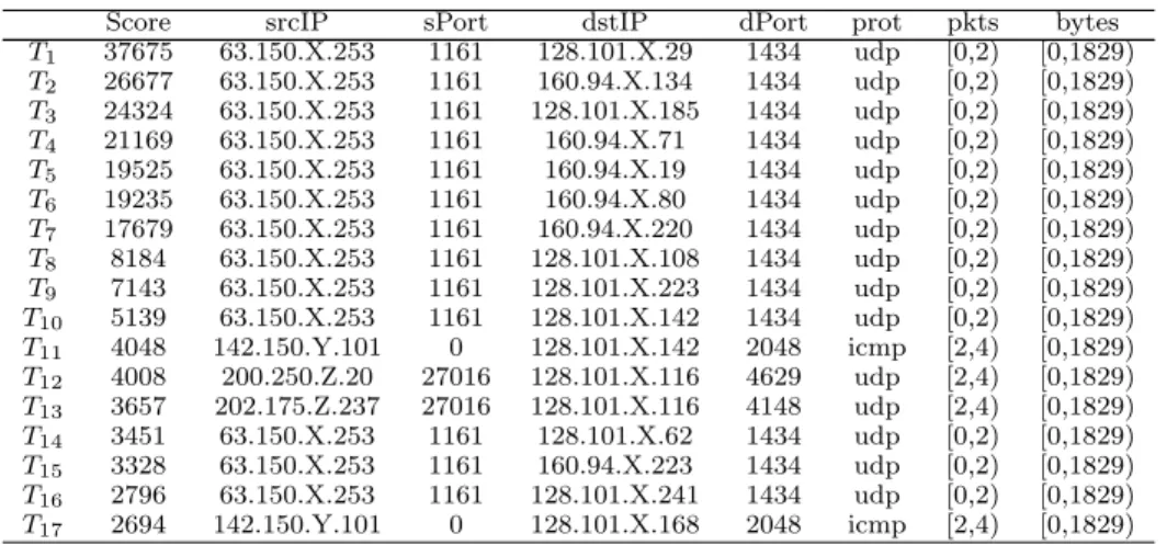
One such application is in the analysis of netflow data to detect cyber attacks. Netflow data is a set of records that describe network traffic, where each record has different features such as the IPs and ports involved, packets and bytes transferred (see Table 1). An important characteristic of netflow data is that it has a mix of categorical and continuous features. The volume of netflow data which a network analyst has to monitor is huge. For example, on a typical day at the University of Minnesota, more than one million flows are collected in every 10 minute window. Manual monitoring of this data is impossible and motivates the need for data mining techniques. Anomaly detection systems [9, 17, 4, 22] can be used to score these flows, and the analyst typically looks at only the most anomalous flows to identify attacks or other undesirable behavior. In a typical window of data being analyzed, there are often several hundreds or thousands of highly ranked flows that require the analyst’s attention. But due to the limited time available, analysts look at only the first few pages of results that cover the top few dozen most anomalous flows. If many of these most anomalous flows can be summarized into a small representation, then the analyst can analyze a much larger set of anomalies than is otherwise possible. For example, Table 2 shows 17 flows which were ranked as most suspicious by the MINDS Anomaly Detection Module [9] for the network traffic analyzed on January 26, 2003 (48 hours after theSlammer Wormhit the Internet) for a 10 minute window that contained 1.8 million flows. These flows are involved in three anomalous activities - slammer worm related traffic on port 1434, flows associated with ahalf-life game server on port 27016 and ping scans of the inside network by an external host on port 2048. If the dataset shown in Table 2 can be automatically summarized into the form shown in Table 3 (the last column has been removed since all the transactions contained the same value for it in Table 2), then the analyst can look at only 3 lines to get a sense of what is happening in 17 flows. Table 3 shows the output summary for this dataset generated by an application of our proposed scheme. We see that every flow is represented in the summary. The first summaryS1represents flows{T1-T10,T14-T16}which correspond to the
slammer worm traffic coming from a single external host and targeting several internal hosts. The second summaryS2represents flows{T12,T13}which are the
1 Traditionally, a centroid is defined as the average of the value of each attribute over all
transactions. If a categorical attribute has different values (say red, blue, green) for three different transactions in the cluster, then it does not make sense to take an average of the values. Although it is possible to replace a categorical attribute with an asymmetric binary attribute for each value taken by the attribute, such methods do not work well when the attribute can take a large number of values, as in the netflow data – see Table 1.
Score srcIP sPort dstIP dPort prot pkts bytes T1 37675 63.150.X.253 1161 128.101.X.29 1434 udp [0,2) [0,1829) T2 26677 63.150.X.253 1161 160.94.X.134 1434 udp [0,2) [0,1829) T3 24324 63.150.X.253 1161 128.101.X.185 1434 udp [0,2) [0,1829) T4 21169 63.150.X.253 1161 160.94.X.71 1434 udp [0,2) [0,1829) T5 19525 63.150.X.253 1161 160.94.X.19 1434 udp [0,2) [0,1829) T6 19235 63.150.X.253 1161 160.94.X.80 1434 udp [0,2) [0,1829) T7 17679 63.150.X.253 1161 160.94.X.220 1434 udp [0,2) [0,1829) T8 8184 63.150.X.253 1161 128.101.X.108 1434 udp [0,2) [0,1829) T9 7143 63.150.X.253 1161 128.101.X.223 1434 udp [0,2) [0,1829) T10 5139 63.150.X.253 1161 128.101.X.142 1434 udp [0,2) [0,1829) T11 4048 142.150.Y.101 0 128.101.X.142 2048 icmp [2,4) [0,1829) T12 4008 200.250.Z.20 27016 128.101.X.116 4629 udp [2,4) [0,1829) T13 3657 202.175.Z.237 27016 128.101.X.116 4148 udp [2,4) [0,1829) T14 3451 63.150.X.253 1161 128.101.X.62 1434 udp [0,2) [0,1829) T15 3328 63.150.X.253 1161 160.94.X.223 1434 udp [0,2) [0,1829) T16 2796 63.150.X.253 1161 128.101.X.241 1434 udp [0,2) [0,1829) T17 2694 142.150.Y.101 0 128.101.X.168 2048 icmp [2,4) [0,1829) Table 2.Top 17 anomalous flows as scored by the anomaly detection module of the MINDS system for the network data collected on January 26, 2003 at the University of Minnesota (48 hours after theSlammer Wormhit the Internet). The third octet of IPs is anonymized for privacy preservation.
Size Score srcIP sPort dstIP dPort prot pkts
S1 13 15102 63.150.X.253 1161 *** 1434 udp [0,2)
S2 2 3833 *** 27016 128.101.X.116 *** udp [2,4)
S3 2 3371 142.150.Y.101 0 *** 2048 icmp [2,4)
Table 3.Summarization output for the dataset in Table 2. The last column has been removed since all the transactions contained the same value for it in the original dataset.
connections made tohalf-lifegame servers made by an internal host. The third summary,S3 represents flows{T11,T17}which correspond to aping scanby the
external host. In general, such summarization has the potential to reduce the size of the data by several orders of magnitude.
In this paper, we address the problem of summarization of data sets that have categorical features. We view summarization as a transformation from a given dataset to a smaller set of individual summaries with an objective of retaining the maximum information content. A fundamental requirement is that every data item should be represented in the summary.
1.1. Contributions
Our contributions in this paper are as follows –
– We formulate the problem of summarization of transactions that contain cate-gorical data, as a dual-optimization problem and characterize a good summary using two metrics – compaction gain and information loss. Compaction gain signifies the amount of reduction done in the transformation from the actual data to a summary. Information loss is defined as the total amount of infor-mation missing over all original data transactions in the summary.
– We investigate two approaches to address this problem. The first approach is an adaptation of clustering and the second approach makes use of frequent itemsets from the association analysis domain [3].
– We present an optimal but computationally infeasible algorithm to generate the best summary for a set of transactions in terms of the proposed metrics.
T1 12.190.84.122 32178 100.10.20.4 80 tcp —APRS- [2,20] [504,1200] T2 88.34.224.2 51989 100.10.20.4 80 tcp —APRS- [2,20] [220,500] T3 12.190.19.23 2234 100.10.20.4 80 tcp —APRS- [2,20] [220,500] T4 98.198.66.23 27643 100.10.20.4 80 tcp —APRS- [2,20] [42,200] T5 192.168.22.4 5002 100.10.20.3 21 tcp —A-RSF [2,20] [42,200] T6 192.168.22.4 5001 100.10.20.3 21 tcp —A-RS- [40,68] [220,500] T7 67.118.25.23 44532 100.10.20.3 21 tcp —A-RSF [40,68] [42,200] T8 192.168.22.4 2765 100.10.20.4 113 tcp —APRS- [2,20] [504,1200] Table 4.A synthetic dataset of network flows.
We also present a computationally feasible heuristic-based algorithm and in-vestigate different heuristics which can be used to generate an approximately good summary for a given set of transactions.
– We illustrate one application of summarization in the field of network data where we show how our technique can be effectively used to summarize network traffic into a compact but meaningful representation. Specifically, we evaluate our proposed algorithms on the 1998 DARPA Off-line Intrusion Detection Evaluation data [15] and network data generated by SKAION Corp for the ARDA information assurance program [1].
2. Characterizing a Summary
Summarization can be viewed as compressing a given set of transactions into a smaller set of patterns while retaining the maximum possible information. A trivial summary for a set of transactions would be itself. The information loss here is zero but there is no compaction. Another trivial summary would be the empty set ², which represents all the transactions. In this case the gain in compaction is maximum but the summary has no information content. A good summary is one which is small but still retains enough information about the data as a whole and also for each transaction.
We are given a set of n categorical features F = {F1, F2, . . . , Fn} and an
associated weight vectorW such that eachWi ∈W represents the weight of the
feature Fi ∈ F. A set of transactions T, such that |T| = m, is defined using
these features, and eachTi ∈ T has a specific value for each of the n features.
Formally, a summary of a set of transactions can be defined as follows:
Definition 1. (Summary) A summary S of a set of transactionsT, is a set of individual summaries{S1, S2, . . . , Sl} such that (i) each Sj represents a subset
ofT and (ii) every transactionTi ∈T is represented by at least oneSj ∈S.
Each individual summarySj essentially covers a set of transactions. In the
sum-maryS, these transactions are replaced by the individual summary that covers them. As we mentioned before, computing the centroid for data with categor-ical attributes is not possible. For such data, a feature-wise intersection of all transactions is a more appropriate description of an individual summary. Hence, from now on, an individual summary will be treated as a feature-wise inter-section of all transactions covered by it, i.e., if Sj covers{T1, T2, . . . , Tk}, then
Sj =
Tk
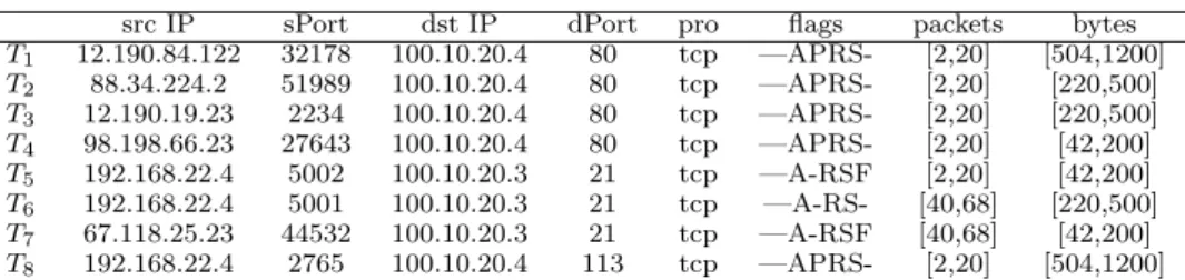
i=1Ti. For the sake of illustration let us consider the sample netflow
data given in Table 4. The dataset shown is a set of 8 transactions that are described by 6 categorical features and 2 continuous features (see Table 1). Let
src IP sPort dst IP dPort pro flags packets bytes
S1 *.*.*.* *** 100.10.20.4 *** tcp —APRS- [2,20] ***
S2 *.*.*.* *** 100.10.20.3 21 tcp *** *** ***
S3 192.168.22.4 2765 100.10.20.4 113 tcp —APRS- [2,20] [504,1200] Table 5.A possible summary for the dataset shown above.
Compaction Gain Information Loss 1 m 0 Optimal Algorithm Algorithm 1 Algorithm 2
Fig. 1.ICC Curve for summarization algorithms
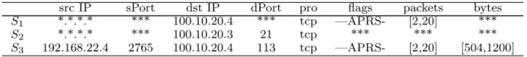
all the features have equal weight of 18. One summary for this dataset is shown in Table 5 as a set of 3 individual summaries. The individual summaryS1covers
transactions {T1,T2,T3,T4,T8}, S2 covers transactions {T5,T6,T7} and S3 covers
only one transaction,T8.
To assess the quality of a summary S of a set of transactions T, we define following metrics
-Definition 2. (Compaction Gain for a Summary) Compaction Gain = m l.
(Recall thatm=|T|andl =|S|.)
For the dataset in Table 4 and the summary in Table 5,Compaction Gain forS = 8
3.
Definition 3. (Information Loss for a transaction represented by an individual summary) For a given transaction Ti ∈T and an individual
sum-marySj ∈ S that coversTi, lossij =
Pn
q=1Wq∗bq, where, bq = 1 if Tiq 6∈Sj
and 0 otherwise.
The loss incurred if a transaction is represented by an individual summary will be the weighted sum of all features that are absent in the individual summary. Definition 4. (Best Individual Summary for a transaction) For a given transactionTi∈T, a best individual summarySj∈Sis the one for whichlossij
is minimum.
The total information loss for a summary is the aggregate of the information lost for every transaction with respect to its best individual summary.
For the dataset in Table 4 and its summary shown in Table 5, transactions T1-T4 are best covered by individual summary S1 and each has an information
loss of 4
8. Transactions T5-T7 are best covered by individual summary S2 and
each has an information loss of 5
8. T8 is represented by S1 andS3. For T8 and S1, information loss = 4×18 = 12, since there are 4 features absent inS1. ForT8
andS3, information loss = 0 since there are no features absent inS3. Hence the
best individual summary forT8 will beS3. Thus, we get that Information Loss
forS = 4
Clustering-based Algorithm Input:T: a transaction data set.
W: a set of weights for the features.
l: size of final summary
Output: S: the final summary.
Variables:C: clusters ofT.
Method:
1. InitializeS={}
2. Run clusteringT to obtain a set oflclusters, ¯C. 3. foreach ¯Ci∈C¯ 4. Si= Tm j=1Cij 5. endfor 6. End
Fig. 2.The Clustering-based Algorithm
It is to be noted that the characteristics, compaction gainand information loss, follow an optimality tradeoff curve as shown in Figure 1 such that increasing the compaction results in increase of information loss. We denote this curve as ICC (Information-loss Compression-gain Characteristic) curve.
The ICC curve is a good indicator of the performance of a summarization algorithm. The beginning and the end of the curve are fixed by the two trivial solutions discussed earlier. For any summarization algorithm, it is desirable that the area under its ICC curve be minimal. It can be observed that getting an optimal curve as shown in Figure 1 involves searching for a solution in exponential space and hence not feasible. But a good algorithm should be close enough to the optimal curve like 1 and not like 2 in the figure shown.
As the ICC curve indicates, there is no global maxima for this dual-optimization problem since it involves two orthogonal objective functions. So a typical objec-tive of a summarization algorithm would be -for a given level of compaction find a summary with the lowest possible information loss.
3. Summarization Using Clustering
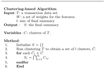
In this section, we present a direct application of clustering to obtain a summary for a given set of transactions with categorical attributes. This simple algorithm involves clustering of the data using any standard clustering algorithm and then replacing each cluster with a representation as described earlier using feature-wise intersection of all transactions in that cluster. The weightsW are used to calculate the distance between two data transactions in the clustering algorithm. Thus, if ¯Cis a set of clusters obtained from a set of transactionsT by clustering, then each cluster produces an individual summary which is essentially the set of feature-value pairs which are present in all transactions in that cluster. The number of clusters here determine the compaction gain for the summary.
Figure 2 gives the clustering based algorithm. Step 2 generates l clusters, while step 3 and 4 generate the summary description for each of the
individ-src IP sPort dst IP dPort protocol flags packets bytes
C1 *.*.*.* *** 100.10.20.4 *** tcp —APRS- [2,20] ***
C2 *.*.*.* *** 100.10.20.3 21 tcp *** *** ***
Table 6.A summary obtained for the dataset in Table 4 using the clustering based algorithm
src IP sPort dst IP dPort protocol flags packets bytes
T9 12.190.84.122 32178 100.10.20.10 53 udp ——– [25,60] [2200,5000] Table 7.An outlying transactionT9 added to the data set in Table 4
ual clusters. For illustration consider again the sample dataset of 8 transac-tions in Table 4. Let clustering generate two clusters for this dataset – C1 =
{T1,T2,T3,T4,T8} and C2 ={T5,T6,T7}. Table 6 shows a summary obtained
us-ing the clusterus-ing based algorithm.
The clustering based approach works well in representing the frequent modes of behavior in the data because they are captured well by the clusters. However, this approach performs poorly when the data has outliers and less frequent pat-terns. This happens because the outlying transactions are forced to belong to some cluster. If a cluster has even a single transaction which is different from other cluster members, it degrades the description of the cluster in the summary. For example, let us assume that another transaction T9 as shown in Table 7 is
added to the dataset shown in Table 4 and clustering assigns it to clusterC1.
On adding T9 to C1, the summary generated from C1 will be empty. The
presence of this outlying transaction makes the summary description very lossy in terms of information content. Thus this approach represents outliers very poorly, which is not desirable in applications such as network intrusion detection and fraud detection where such outliers can be of special interest.
4. An Optimal Summarization Algorithm
In this section we propose an exhaustive search algorithm (shown in Figure 3) which is guaranteed to generate an optimal summary of given sizel for a given set of transactions, T. The first step of this algorithm involves generating the powerset ofT (= all possible subsets ofT), denoted byC. The size ofC will be 2|T|. The second step involves searching all possible subsets ofC (22|T|
subsets) to select a subset,S which has following properties
Property 1.
(1) |S|=l, the size of this subset is equal to desired compaction level (2) The subsetS covers all transactions inT (a set cover ofT)
(3) The total information loss forS with respect toT is minimum over all other subsets ofT which satisfy the properties 1 and 2
We denote the optimal summary generated by the algorithm in Figure 3 byS. The optimal algorithm follows the optimal ICC curve as shown in Figure 1.
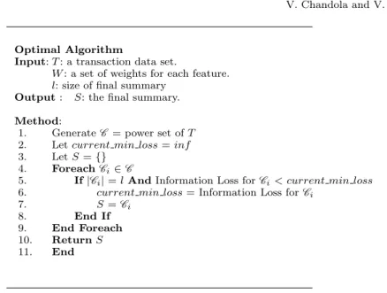
Optimal Algorithm
Input:T: a transaction data set.
W: a set of weights for each feature.
l: size of final summary
Output: S: the final summary.
Method:
1. GenerateC = power set ofT
2. Letcurrent min loss=inf
3. LetS={}
4. ForeachCi∈C
5. If|Ci|=lAndInformation Loss forCi< current min loss
6. current min loss= Information Loss forCi
7. S=Ci
8. End If
9. End Foreach
10. ReturnS
11. End
Fig. 3.The Optimal Algorithm
5. A Two-step Approach to Summarization using
Frequent Itemsets
The optimal algorithm presented in Section 4 requires searching in a 22|T|
space (for 4 transactions it would require searching a set of 65,536 subsets), which makes it computationally infeasible even for very small data sets. In this section we propose a methodology which simplifies each of the two steps of the optimal algorithm to make them computationally more efficient. We first present the fol-lowing lemma.
Lemma 1. Any subset ofT belonging to the optimal summary,S must belong toCc, whereCc denotes a set containing allclosedfrequent itemsets2 generated
with a support threshold of 2 andT itself.
Proof. This can be easily proved by contradiction. Suppose the optimal sum-mary contains a subsetSi ∈C -Cc. Thus there will be a subsetSj ∈Cc which
“closes”Si, which meansSj⊃Siandsupport(Si) =support(Sj). We can replace
Si with Sj in S to obtain another summary,S0 such that all the transactions
represented bySi in S are represented by Sj in S0. SinceSj ⊃Si, the
infor-mation loss for these transactions will be lower inS0. Thus S0 will have lower information loss thanS for the same compaction which is not possible sinceS
is an optimal summary.
We modify the Step 1 of optimal algorithm in Figure 3 and replace C with Cc. The result from Lemma 1 ensures that we can still obtain the optimal
sum-mary from the reduced candidate set. But to obtain an optimal solution we still
2 An itemset X is a closed itemsetif there exists no proper supersetX0 ⊃X such that support(X0) =support(X).
need to search from the powerset ofCc, which is still computationally infeasible.
Higher values of the support threshold can be used to further prune the number of possible candidates, but this can impact the quality of the summaries obtained. We replace the Step 2 of optimal algorithm with agreedy searchwhich avoids the exponential search by greedily searching for a good solution. This does not guarantee the optimal summary but tries to follow the optimal ICC curve (refer to Figure 1). The output (a subset ofCc) of Step 2 of our proposed algorithms
satisfiy Property 1.1 and Property 1.2 mentioned in Section 4 but is not guar-anteed to satisfy Property 1.3.
The selection of a subset of Cc such that its size satisfies the desired
com-paction level while the information loss associated with this subset is approxi-mately minimal can be approached in two ways.
– The first approach works in a top-down fashion where every transaction be-longing to T selects a “best” candidate for itself (based on a heuristic based function which will be described in later in this section ). The union of all such candidates is the summary forT.
– The second approach works in abottom-upfashion by starting with T as the initial summary and choosing a “best” candidate at every step and adding it to the summary. The individual summaries that are covered by the chosen candidates are replaced, thereby causing compaction.
In this paper we will discuss only the bottom-up approach for summarization. An algorithm based on thetop-downapproach is presented in an extended tech-nical report [8]. Both of these approaches build a summary in an iterative and incremental fashion, starting from the original set of transactionsT as the sum-mary. Thus from the ICC curve perspective, they start at the left hand corner (compaction=1,loss=0). At each iteration the compaction gain increases along with the information loss. Each iteration makes the current summary smaller by bringing in one or more candidates into the current summary.
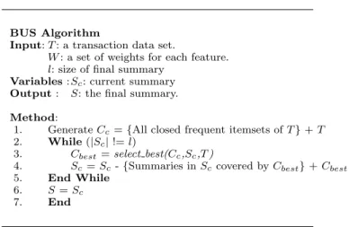
6. A Bottom-up Approach to Summarization - The BUS
Algorithm
The main idea behind the BUS algorithm is to incrementally select best can-didates from the candidate set such that at each step, for a certain gain in compaction, minimum information loss is incurred. The definition of a “best” candidate is based on a heuristic decision and can be defined in several different ways as we will describe later.
Figure 4 presents a generic version of BUS. Line 1 involves generation of all closed frequent itemsets ofT. As mentioned earlier, choosing a support threshold of 2 transactions while generating the frequent itemsets as well as the transac-tions themselves ensures that we capture patterns of every possible size. The rest of the algorithm works in an iterative mode until a summary of desired compaction level l is obtained. In each iteration a candidate from Cc is chosen
using the routine select best. We have investigated several heuristic versions of select bestwhich will be described later. The general underlying principle for de-signing aselect best routine is to ensure that the selected candidate incurs very
BUS Algorithm
Input:T: a transaction data set.
W: a set of weights for each feature.
l: size of final summary
Variables:Sc: current summary Output: S: the final summary.
Method:
1. GenerateCc={All closed frequent itemsets ofT}+T
2. While(|Sc|!=l)
3. Cbest=select best(Cc,Sc,T)
4. Sc=Sc-{Summaries inSccovered byCbest}+Cbest
5. End While
6. S=Sc
7. End
Fig. 4.The Generic BUS Algorithm
low information loss while reducing the size of summary. After choosing a best candidate, Cbest, all individual summaries in current summary which are
com-pletely covered3 by C
best are removed and Cbest is added to the summary (let
the new summary be denoted byS0
c).
Thus after each iteration, the size of the summary,Scis reduced bysize(Cbest)
- 1, where size(Cbest) denotes the number of individual summaries in Sc
com-pletely covered by Cbest. This is denoted by gain(Ci, Sc) and represents the
compaction gain achieved by choosing candidateCi for a given summarySc.
For computing the loss incurred by addingCbestto the current summary (and
replacing the summaries covered byCbest), we need to consider the transactions
which will considerCbest as theirbest individual summary(refer to Definition 4)
in the new summary. For all such transactions, the difference in the loss when they were represented inScby theirbest individual summariesand the loss when
they are represented byCbest inS0c is the extra loss incurred in choosingCbest.
This is denoted byloss(Ci, Sc).
Next we describe four different ways in which function select best can be designed. Each of these approaches make a greedy choice to choose a candidate from the current candidate setCc which would lead to alocally optimal solution
but does not ensure that the sequence of these choices will lead to a globally optimal solution.
6.1. Method 1
This method (as shown in Figure 5) uses the quantitiesgain(Ci, Sc) andloss(Ci, Sc),
defined above, to score the candidates and choose one to be added to the cur-rent summary, Sc. All candidates withgain(Ci, Sc) equal to or less than 1 are
3 An individual summary is completely covered by a candidate if it is more specific than the
select best - Method 1 Input:T: a transaction data set.
Sc: current summary.
Cc: candidate set. Output: Cbest: best candidate. Method:
1. min-loss= minimum(loss(Ci, Sc),∀Ci∈Cc&gain(Ci, Sc)>1)
2. C0 ={C
i|Ci∈Cc&gain(Ci, Sc)>1 &loss(Ci, Sc) =min-loss}
3. best=argmaxCi∈C0(gain(Ci, Sc)) 4. returnCbest
5. End
Fig. 5.select best- Method 1
ignored (since adding them to the current summary would not result in any com-paction gain in the new summary). The remaining candidates are ordered using loss(Ci, Sc). From among the candidates which have lowest value forloss(Ci, Sc),
the candidate with highestgain(Ci, Sc) is returned as thebest candidate.
Thus this approach tries to maintain a very low information loss at each iteration by bringing in the candidates with lowest information loss.
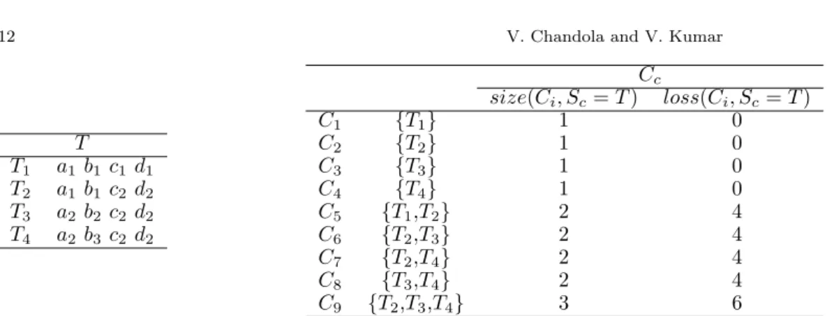
But as mentioned above, the decision to pick up a candidate in this manner might eventually result in a sub-optimal solution. A simple counter-example shown in Figure 6 proves this. Let us consider a simple data set which has four transactions{T1,T2,T3,T4}defined over four attributes{a,b,c,d}(each attribute
has a unit weight). The aim is to obtain a summary of size 2 for this data set using the BUS algorithm. As shown in the figure, the candidate setCc contains
9 possible candidates. The BUS algorithm considers the transaction set, T as the initial summary, Sc. The first iteration uses method 1 and (see Figure 7)
chooses candidateC5as the best candidate, generating a newSc. The candidate
set is rescored as shown in the figure. The next iteration chooses (see Figure 7) C9 as the best candidate and reduces the size of Sc to 2. The right side table
in Figure 7 shows another size 2 summary for the same data set which has a smaller information loss. This shows that this method to score candidates might not result in an optimal solution.
6.2. Method 2
This method (as shown in Figure 9) also uses the quantities gain(Ci, Sc) and
loss(Ci, Sc) as in Method 1, but in a different way. All candidates withgain(Ci, Sc)
equal to or less than 1 are ignored (since adding them to the current summary would not result in any compaction gain in the new summary). The remaining candidates are ordered using gain(Ci, Sc). From among the candidates which
have lowest value for gain(Ci, Sc), the candidate with lowestloss(Ci, Sc) is
re-turned as thebest candidate.
This method is symmetrically opposite to method 1 and makes use of the symmetry betweeninformation loss andcompaction gain. The general idea be-hind method 2 is that at any iteration, the candidates which cover least number of individual summaries in the current summarySc, will also incur the lowest
T T1 a1 b1 c1 d1 T2 a1 b1 c2 d2 T3 a2 b2 c2 d2 T4 a2 b3 c2 d2 Cc size(Ci, Sc=T) loss(Ci, Sc =T) C1 {T1} 1 0 C2 {T2} 1 0 C3 {T3} 1 0 C4 {T4} 1 0 C5 {T1,T2} 2 4 C6 {T2,T3} 2 4 C7 {T2,T4} 2 4 C8 {T3,T4} 2 4 C9 {T2,T3,T4} 3 6
Fig. 6.Left- A simple data set,T with 4 transactions defined over 4 features. Each feature is assumed to have a unit weight.Right- The candidate set,Ccwithgain(Ci, Sc) andloss(Ci, Sc)
defined for current summary,Sc=T.
Sc C5 a1 b1 T3 a2 b2 c2 d2 T4 a2 b3 c2 d2 Cc size(Ci, Sc) loss(Ci, Sc) C8 {T3,T4} 2 4 C9 {T2,T3,T4} 2 4
Fig. 7.Left- Current summary,Sc after first iteration.Right- The candidate set,Cc after
rescoring based onSc(Showing only the candidates withgain(Ci, Sc)>1).
Sc C5 a1 b1 C8 c2d2 S0 c C1 a1 b1 c1 d1 C9 c2 d2
Fig. 8. Left- Current summary,Sc after second iteration (Size = 2, Information Loss = 8). Right- The optimal summaryS0
c(Size = 2, Information Loss = 6).
select best - Method 2 Input:T: a transaction data set.
Sc: current summary.
Cc: candidate set. Output: Cbest: best candidate. Method:
1. min-gain= minimum(gain(Ci, Sc),∀Ci∈Cc&gain(Ci, Sc)>1)
2. C0={C
i|Ci∈Cc&gain(Ci, Sc)>1 &gain(Ci, Sc) =min-gain}
3. best=argminCi∈C0(loss(Ci, Sc)) 4. returnCbest
5. End
Fig. 9.select best- Method 2
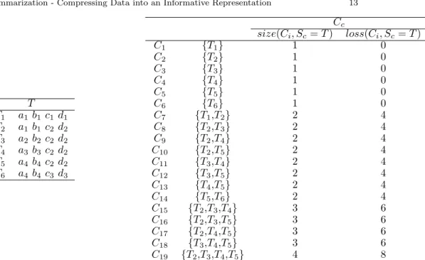
does not guarantee a globally optimal summary. Consider the transaction data set containing 6 transactions as shown in Figure 10. Figures 11-13 show the working of the BUS algorithm using method 2 to obtain a summary of size 3 for this data set. Figure 13(right) shows an alternative summary S0
c, which is of
T T1 a1 b1 c1 d1 T2 a1 b1 c2 d2 T3 a2 b2 c2 d2 T4 a3 b3 c2 d2 T5 a4 b4 c2 d2 T6 a4 b4 c3 d3 Cc size(Ci, Sc=T) loss(Ci, Sc=T) C1 {T1} 1 0 C2 {T2} 1 0 C3 {T3} 1 0 C4 {T4} 1 0 C5 {T5} 1 0 C6 {T6} 1 0 C7 {T1,T2} 2 4 C8 {T2,T3} 2 4 C9 {T2,T4} 2 4 C10 {T2,T5} 2 4 C11 {T3,T4} 2 4 C12 {T3,T5} 2 4 C13 {T4,T5} 2 4 C14 {T5,T6} 2 4 C15 {T2,T3,T4} 3 6 C16 {T2,T3,T5} 3 6 C17 {T2,T4,T5} 3 6 C18 {T3,T4,T5} 3 6 C19 {T2,T3,T4,T5} 4 8
Fig. 10.Left- A simple data set,T with 6 transactions defined over 4 features. Each feature is assumed to have a unit weight.Right- The candidate set,Ccwithgain(Ci, Sc) andloss(Ci, Sc)
defined for current summary,Sc=T.
Sc C7 a1 b1 T3 a2 b2 c2 d2 T4 a3 b3 c2 d2 T5 a4 b4 c2 d2 T6 a4 b4 c3 d3 Cc size(Ci, Sc) loss(Ci, Sc) C11 {T3,T4} 2 4 C12 {T3,T5} 2 4 C13 {T4,T5} 2 4 C14 {T5,T6} 2 4 C15 {T2,T3,T4} 2 4 C16 {T2,T3,T5} 2 4 C17 {T2,T4,T5} 2 4 C18 {T3,T4,T5} 3 6 C19 {T2,T3,T4,T5} 3 6
Fig. 11.Left- Current summary,Scafter first iteration.Right- The candidate set,Ccafter
rescoring based onSc(Showing only the candidates withgain(Ci, Sc)>1).
Sc C7 a1 b1 C11 c2 d2 T5 a4 b4 c2 d2 T6 a4 b4 c3 d3 Cc size(Ci, Sc) loss(Ci, Sc) C14 {T5,T6} 2 4 C18 {T3,T4,T5} 2 2 C19 {T2,T3,T4,T5} 2 2
Fig. 12.Left- Current summary,Scafter second iteration.Right- The candidate set,Ccafter
rescoring based onSc(Showing only the candidates withgain(Ci, Sc)>1).
Sc C7 a1 b1 C18 c2 d2 T6 a4 b4 c3 d3 S0 c T1 a1 b1 c1 d1 C19 c2 d2 T6 a4 b4 c3 d3
Fig. 13.Left- Current summary,Scafter third iteration (Size = 3, Information Loss = 10). Right- The optimal summaryS0
select best - Method 3 Input:T: a transaction data set.
Sc: current summary.
Cc: candidate set.
ks: scoring parameter.
δ: increment parameter forks. Output: Cbest: best candidate. Method:
1. foreachCiinCc
2. score(Ci, Sc) =ks*gain(Ci, Sc) -loss(Ci, Sc)
3. end for
4. max-score= maximum(score(Ci, Sc),∀Ci∈Cc)
5. foreachCiinCc
6. if((score(Ci, Sc) ==max-score) & (gain(Ci, Sc)>1))
7. returnCbest=Ci 8. end if 9. end for 10. ks =ks +δ 11. Goto 1 12. End
Fig. 14.select best- Method 3
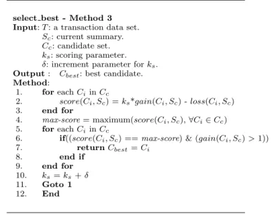
6.3. Method 3
The third method to determine the best candidate makes use of a parameter ks, which combines the two quantitiesgain(Ci, Sc) andloss(Ci, Sc) to obtain a
single value, denoted byscore(Ci, Sc). The method is shown in Figure 14. The
first step calculates the score for each candidate using ks. The candidate with
highest score is chosen as thebestcandidate. Initiallyks is chosen to be 0. This
favors the candidates with very small information loss. If all candidates with the highest score havesize(Ci, Sc) <= 1, then ks is incremented by a small value,
δ. This allows larger candidates to have higher score by offsetting the larger information loss associated with them, and thus be considered for selection into the summary.
The value of ks can be initialized to a value greater than 0, which would
result in selection of larger candidates initially. Using this method again does not guarantee an optimal solution and depends on the initial value ofksandδ.
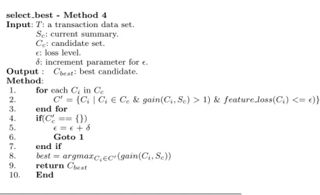
6.4. Method 4
Each of the above three methods require the rescoring ofgain(Ci, Sc) andloss(Ci, Sc)
for each candidate after each iteration. The method 4, shown in Figure 15 does not require these computations but makes use of the quantityf eature loss(Ci)
which refers to the weighted sum of the features missing in a candidate. Note that this quantity does not change over the iterations and hence is computed only once. The method to determine the best candidate uses parameter², which defines a upper threshold onf eature loss(Ci). Only those candidates which have
f eature loss(Ci) less than or equal to this threshold are considered for selection.
select best - Method 4 Input:T: a transaction data set.
Sc: current summary.
Cc: candidate set.
²: loss level.
δ: increment parameter for².
Output: Cbest: best candidate. Method:
1. foreachCiinCc
2. C0={C
i|Ci∈Cc&gain(Ci, Sc)>1) &f eature loss(Ci)<=²)}
3. end for 4. if(C0 c=={}) 5. ²=²+δ 6. Goto 1 7. end if
8. best=argmaxCi∈C0(gain(Ci, Sc)) 9. returnCbest
10. End
Fig. 15.select best- Method 4
the best candidate. Initially² is chosen as 0. Thus only candidates with 0 fea-tures missing are considered. If all candidates which fall under²threshold have gain(Ci, Sc)≤ 1, then ² is incremented by a small value, δ. This allows larger
candidates to be considered for selection into the summary.
6.5. Discussion
All the four methods discussed above select a candidate which they consider is the best with respect to a heuristic. We presented examples for first two methods where this choice might not always lead to aglobally optimal solution. The last two methods make use of a user defined parameter and a wrong choice of this parameter can lead to suboptimal solutions. We have investigated each of these approaches and evaluated them on different network data sets (described in next section) and observed that all of them perform comparably in terms of the ICC curve characteristics with respect to each other.
7. Experimental Evaluation And Results
In this section we present the performance of our proposed algorithms on network data. We compare the performance of BUS with the clustering based approach to show that it performs better in terms of achieving lower information loss for a given degree of compaction. As we had mentioned earlier, the clustering based algorithm captures the clusters in the data and summarizes the transactions belonging to those clusters well. But the presence of infrequent patterns can ruin the cluster descriptions and result in high information loss. The experimental results presented in this section highlight this fact by choosing different data sets which have different characteristics in terms of the natural clustering in the data. We also illustrate the summaries obtained for different algorithms to
AD1 1000 Artificially Generated Contains 5 clusters with 200 identical transactions in each cluster
AD2 1100 Artificially Generated For each cluster in AD1 20 transac-tions different in exactly one feature are added
SKAION 8459 SKAION Data set, Scenario S29 Contains normal traffic belonging to natural clusters mixed with outlying attack traffic
DARPA 2903 DARPA Data set, 6 different attack re-lated traffic from training week 4, day 5 data
Most of the transactions belonged to clusters corresponding to each of the larger attacks while some were outliers
Table 8.Description of the different datasets used for experiments.
make a qualitative comparison between them. The algorithms were implemented in GNU-C++ and were run on the Linux platform on a 4-processor intel-i686 machine.
7.1. Input Data
We ran our experiments on four different artificial datasets as listed in Table 8. The first two data sets,AD1 and AD2 were artificially generated such that they contained 5 clusters such that each cluster contained the same transaction replicated 200 times. AD1 contained only these pure clusters. AD2 contained outliers injected with respect to each of the cluster. The SKAION and DARPA data sets were generated by DARPA [15] and SKAION corporation [1] respec-tively, for the evaluation of intrusion detection systems. The DARPA dataset is publicly available and has been used extensively in the data mining community as it was used in KDD Cup 1999. The SKAION data was developed as a part of the ARDA funded program on information assurance and is available only to the investigators involved in the program. Both these datasets have a mixture of normal and attack traffic. The DARPA data set was a subset of the week 4, Friday, training data containing only attack related traffic corresponding to the following attacks -warezclient, rootkit, ffb, ipsweep, loadmodule andmultihop.
All of these datasets exhibit different characteristics in terms of data distrib-ution. We measure the distribution of the data using thelof(local outlier factor) score (see [6]). The distribution forlofscores forAD1 data set is shown in Figure 16(a). Since all transactions belong to one of the 5 clusters, all transactions have a lof score of 1. Similar plot for data setAD2 in Figure 17(a) shows that some of the transactions have a higherlof score since they are outliers with respect to the clusters. Figure 18(a) gives the distribution of the lof (local outlier fac-tor) score (see [6]) for the transactions in the SKAION dataset. The lof score reflects the outlierness of a transaction with respect to its nearest neighbors. The transactions which belong to tight clusters tend to have lowlofscores while outliers have highlofscores. For the SKAION dataset we observe that there are a lot of transactions which have high outlier scores. Thelof distribution for the DARPA dataset in Figure 18(e) shows that most of the transactions belong to tight clusters, and only a few transactions are outliers.
feature name weight Source IP 3.5 Source Port 0 Destination IP 3.5 Destination Port 2 Protocol 0.1 Time to Live(ttl) 0.1 TCP Flags 0.1 Number of Packets 0.3 Number of Bytes 0.3 Window Size 0.1
Table 9.Different features and their weights used for experiments.
7.2. Comparison of ICC curves for the clustering-based
algorithm and BUS
We ran the clustering based algorithm by first generating clusters of different sizes using theCLUTOhierarchical clustering package [14]. For finding the sim-ilarity between transactions, the features were weighted as per the scheme used for evaluating the information loss incurred by a summary. We then summarized the clusters as explained in Section 3. For BUS, we present the results using frequent itemsets generated by theapriori algorithm with a support threshold of 2 as the candidates. The BUS algorithm was executed using method 1 (see Section 6.1)4. The different features in the data and the weights used are given
in Table 9. These weights reflect the typical relative importance given to the different features by network analysts. The continuous attributes in the data were discretized usingequal depth binning technique with a fixed number of in-tervals (= 75) and then used as categorical attributes. Figures 16(b) and 17(b) show the ICC curves for the clustering-based algorithm and BUS on data sets AD1 and AD2 respectively. Since AD1 contains 5 pure clusters, both schemes show no information loss till the compaction gain is 200 (summary size = 5). For compaction more than 200, the information loss increases sharply, since the 5 clusters were chosen to be distinct from each other. Hence no larger summary could be found which could merge any two clusters efficiently. In the second data setAD2, there are 100 outlying transactions. The figure shows that the perfor-mance of the clustering based approach degrades rapidly as the compaction gain is increased. This happens because some of the outlying transactions are forced to belong to the natural clusters, which makes the cluster description very lossy, and hence incurs a large information loss for all members of that cluster.
Figures 18(b) and 18(f) show the ICC curves for the clustering-based algo-rithm and BUS on the DARPA and SKAION data sets respectively. From the two graphs we can see that BUS performs better than the clustering-based ap-proach. We also observe that the difference in the curves for each case reflects thelofscore distribution for each dataset. In the SKAION dataset there are a lot of outliers which are represented poorly by the clustering-based approach while BUS handles them better. Hence the difference in the information loss is very high. In the DARPA dataset, most of the transactions belong to well-defined clusters which are represented equally well by both the algorithms. Thus, the
4 The results from running BUS with other methods were also comparable with this method
0 200 400 600 800 1000 1 2 3 4 5 6 7 8 9 10 Number of flows lof score Artificial Data Set AD1(Size = 1000)
Number of flows 0 1000 2000 3000 4000 5000 6000 7000 8000 9000 0 50 100 150 200 250 300 350 400 450 500
Total Information Loss
Compaction Artificial Data Set AD1(Size = 1000)
clustering based BUS-itemsets
(a) (b)
Fig. 16.(a). Distribution oflofscores for theAD1 data set. (b). ICC curves using the clustering based algorithm and BUS(method 1) on artificial datasetAD1
0 200 400 600 800 1000 1200 1 2 3 4 5 6 7 8 9 10 Number of flows lof score Artificial Data Set AD2(Size = 1100)
Number of flows 0 1000 2000 3000 4000 5000 6000 7000 8000 9000 10000 0 50 100 150 200 250
Total Information Loss
Compaction Artificial Data Set 2(Size = 1100)
clustering based BUS-itemsets
(a) (b)
Fig. 17.(a). Distribution oflofscores for theAD2 data set. (b). ICC curves using the clustering based algorithm and BUS(method 1) on artificial dataset AD2
difference in information loss for the two algorithms is not very high in this case. To further strengthen our argument that clustering tends to ignore the infre-quent patterns and outliers in the data, we plot the information loss for transac-tions which have lost a lot of information in the summary. Figure 18(c) shows the difference in the ICC curves for the transactions in the DARPA dataset which have lost more than 70% information. The graph shows that for BUS, none of the transactions lose more than 70% information till a compaction gain of about 220, while for the clustering based approach, there are considerable number of transactions which are very poorly represented even for a compaction gain of 50. A similar result for the SKAION dataset in Figure 18(g) shows that BUS generates summaries in which very few transactions have a high loss, which is not true in the case of the clustering based approach.
Figure 18(d) shows the difference in the ICC curves for each algorithm for the transactions which have lost less than 70% of information for the DARPA dataset. This plot illustrates the difference in behavior of the two algorithms in terms of summarizing the transactions which belong to some frequent pattern in the data. The clustering based approach represents these transactions better
0 500 1000 1500 2000 2500 1 2 3 4 5 6 7 8 9 10 Number of flows lof score Distribution of lof scores for flows in DARPA Dataset
DARPA Dataset 0 5000 10000 15000 20000 25000 0 50 100 150 200 250 300 350 Information Loss Compaction Gain DARPA Dataset (size = 2903 flows)
BUS-itemsets clustering based 0 2000 4000 6000 8000 10000 12000 14000 16000 18000 0 50 100 150 200 250 300 350 >70% Information Loss Compaction Gain DARPA Dataset (size = 2903 flows)
BUS-itemsets clustering based 0 2000 4000 6000 8000 10000 12000 14000 16000 18000 20000 0 50 100 150 200 250 300 350 <70% Information Loss Compaction Gain DARPA Dataset (size = 2903 flows)
BUS-itemsets clustering based (a) (b) (c) (d) 0 500 1000 1500 2000 2500 3000 3500 1 2 3 4 5 6 7 8 9 10 Number of flows lof score Distribution of lof scores for flows in SKAION Dataset
SKAION Dataset 0 10000 20000 30000 40000 50000 60000 70000 80000 90000 0 200 400 600 800 1000 1200 1400 1600 1800 Information Loss Compaction Gain SKAION Dataset (size = 8459 flows)
BUS-itemsets clustering based 0 10000 20000 30000 40000 50000 60000 70000 80000 0 200 400 600 800 1000 1200 1400 1600 1800 >70% Information Loss Compaction Gain SKAION Dataset (size = 8459 flows)
BUS-itemsets clustering based 0 5000 10000 15000 20000 25000 30000 35000 40000 0 200 400 600 800 1000 1200 1400 1600 1800 <70% Information Loss Compaction Gain SKAION Dataset (size = 8459 flows)
BUS-itemsets clustering based
(e) (f) (g) (h)
Fig. 18.Figures (a) – (d) present results for the DARPA dataset, Figures (e) – (h) present results for SKAION dataset. (a,e) Distribution oflofscores. (b,f) ICC Curve for the clustering based algorithms and BUS. (c,g) Sum of the Information Loss for transactions that have lost more than 70% of information. (d,h) Sum of the Information Loss for transactions that have lost less than 70% information.
than BUS. A similar result can be seen for the SKAION dataset in Figure 18(h).
7.3. Qualitative Analysis of Summaries
In this section we illustrate the summaries obtained by running the clustering based algorithm (see Table 10), and BUS using frequent itemsets (see Table 11) on the DARPA dataset described above. This dataset is comprised of different attacks launched on the internal network by several external machines. The tables do not contain all the features due to the lack of space. However, the information loss was computed using all the features shown in Table 9.
In the summary obtained from the clustering based approach, we observe that S1 andS3 correspond to the icmpand udptraffic in the data. Summaries S2, S4 andS6represent the ftptraffic on port 20, corresponding to thewarezclient,
loadmoduleandffbattacks which involve illegalftptransfers.S5represents traffic
on port 23 which correspond to therootkitandmultihopattacks. The rest of the summaries,S7-S10, do not have enough information as most of the features are
missing. These cover most of the infrequent patterns and the outliers which were ignored by the clustering algorithm. Thus we see that the clustering based algorithm manages to bring out only the frequent patterns in the data. The summary obtained from BUS gives a much better representation of the data. Almost all the summaries in this case contain one of the IPs (which have high weights), which is not true for the output of the clustering-based algorithm. Summaries S1 andS2 represent theffb and loadmodule attacks since they are
launched by the same source IP. Thewarezclientattack on port 21 is represented byS3. Theipsweepattack, which is essentially a single external machine scanning
a lot of internal machines on different ports, is summarized inS6.S5summarizes
the connections which correspond to internal machines which replied to this scanner. The real advantage of this scheme can be seen if we observe summaryS9
S1 513 *** 0 *** 0 icmp [1,1] [28,28] S2 51 172.16.112.50 20 *** *** tcp *** *** S3 119 *** *** *** *** udp *** *** S4 362 197.218.177.69 20 *** *** tcp [5,5] *** S5 141 *** *** *** 23 tcp *** *** S6 603 172.16.114.148 20 *** *** tcp *** *** S7 507 *** *** *** *** tcp *** *** S8 176 *** *** *** *** tcp *** *** S9 249 *** *** *** *** tcp *** *** S10 182 *** *** *** *** tcp *** ***
Table 10.A size 10 summary obtained for DARPA dataset using the clustering based algo-rithm. Information Loss=23070.5
size src IP sPort dst IP dPort proto packets bytes
S1 279 *** *** 135.13.216.191 *** *** *** *** S2 364 135.13.216.191 *** *** *** *** *** *** S3 138 *** *** *** 21 tcp *** *** S4 76 172.16.112.50 *** *** *** *** *** *** S5 249 *** *** 197.218.177.69 *** *** *** *** S6 1333 197.218.177.69 *** *** *** *** *** *** S7 629 172.16.114.148 *** *** *** tcp *** *** S8 153 *** *** *** 23 tcp *** *** S9 1 172.16.114.50 23 207.230.54.203 1028 tcp [1,1] [41,88] S10 5 *** 0 197.218.177.69 0 icmp [1,1] [28,28]
Table 11.A size 10 summary obtained for DARPA dataset using BUS algorithm. Information Loss=18601.7
which is essentially a single transaction. In the data, this is the only connection between these two machines and corresponds to the rootkit attack. The BUS algorithm preserves this outlier even for such a small summary because there is no other pattern which covers it without losing too much information. Similarly, S10 represents 5 transactions which are icmp replies to an external scanner by
5 internal machines. Note that these replies were not merged with the summary S5but were represented as such. Thus, we see that summaries generated by BUS
algorithm represent the frequent as well as infrequent patterns in the data.
8. Related Work
Compression techniques such aszip, mp3, mpeg etc.also aim at reduction in data size. But compression techniques are motivated by system constraints such as processor speed, bandwidth and disk space. Compression schemes try to reduce the size of the data for efficient storage, processing or data transfer. Summa-rization, on the other hand, aims at providing an overview of the data, thereby allowing an analyst to get an idea about the data without actually having to analyze the entire data.
Many researchers have addressed the issue of finding a compact representa-tion of frequent itemsets [2, 20, 11, 19, 7, 5]. However, their final objective is to approximate a collection of frequent itemsets with a smaller subset, which is different from the problem addressed in this paper, in which we try to represent a collection of transactions with a smaller summary.
commu-nity, and has been addressed mostly as a natural language processing problem which involves semantic knowledge and is different from the problem of rization of transaction data addressed in this paper. Another form of summa-rization is addressed in [12] and [16], where the authors aim at organizing and summarizing individual rules for better visualization while not addressing the issue of summarizing the data.
The closest related work on summarization of categorical data sets is by Wang and Karypis [24]. This paper proposes an algorithm (SUMMARY) to find a set of frequent itemsets (based on a support threshold), which is called a summary-set, for a given set of transactions. The summary-set is found by determining the longest frequent itemset which covers a transaction, for each transaction and then taking union of all such longest frequent itemsets. Thesummary-setis then used to determine clusters for the given data set by treating each member of the summary-set as a cluster such that all transactions which considered that member as their longest representation belong to the same cluster. The authors claim that the summary-set determined using the SUMMARY algorithm is a good summary of the entire data set. Indeed this method can be viewed as one instance of the top-down approach for computing summaries. However there are several shortcomings associated with it as discussed below
– Thesummary-setdoes not guarantee to cover every transaction belonging to the data set. Outlying transactions which do not match with any other trans-action on any feature will not exist in any frequent itemset (even if the support threshold is 2 transactions). Such transactions will not have any representa-tive in the summary-set and will be completely lost. This would be highly undesirable in applications where outliers are of great significance to analysts. As mentioned in the introduction, every transaction has to have some form of representation in the final summary. We must note that the real objective of thesummary-setalgorithm (as stated in the paper) is to find clusters. – This method does not try to explicitly trade-off compaction gain for
infor-mation loss. The compaction gain is very indirectly controlled by the support threshold parameter. Thus to reduce the size of summary-set, the support threshold can be increased. But this would result in more and more infrequent transactions getting completely lost.
9. Concluding Remarks and Future Work
The two schemes presented for summarizing transaction datasets with categor-ical attributes demonstrated their effectiveness in the context of network traffic analysis. A variant of our proposed two-step approach is used routinely at the University of Minnesota as a part of the MINDS system to summarize several thousand anomalous netflows into just a few dozen summaries. This enables the analyst to visualize the suspicious traffic in a concise manner and often leads to the identification of attacks and other undesirable behavior that cannot be captured using widely used intrusion detection tools such as SNORT.
The summarization techniques presented in this paper assume that all trans-actions in the data set are equally important. In several applications, the transac-tions might have different levels of importance. In such cases it will be desirable for higher ranked transactions to incur low information loss while lower ranked transactions can tolerate a little higher information loss.
A typical example can be found in network anomaly detection domain where the network flows are ranked based on their anomaly scores. The main challenge that arises in adapting our proposed summarization techniques to this problem is how to incorporate the knowledge of ranks while scoring the candidates to achieve the above stated objective. We are currently investigating a few possible approaches in this direction.
Acknowledgements
The authors thank Gaurav Pandey and Shyam Boriah for their extensive com-ments on an earlier draft of the paper.
This work was supported by Army High Performance Computing Research Center contract number DAAD19-01-2-0014, by the ARDA Grant AR/F30602-03-C-0243 and by the NSF grant IIS-0308264. The content of this work does not necessarily reflect the position or policy of the government and no official endorsement should be inferred. Access to computing facilities was provided by the AHPCRC and the Minnesota Supercomputing Institute.
References
[1] Skaion corporation. skaion intrusion detection system evaluation data, 2003.
[2] F. Afrati, A. Gionis, and H. Mannila. Approximating a collection of frequent sets. In
Proceedings of the 2004 ACM SIGKDD international conference on Knowledge discovery and data mining, pages 12–19, New York, NY, USA, 2004. ACM Press.
[3] R. Agrawal, T. Imieliski, and A. Swami. Mining association rules between sets of items in large databases. InProceedings of the 1993 ACM SIGMOD international conference on Management of data, pages 207–216. ACM Press, 1993.
[4] D. Barbara, J. Couto, S. Jajodia, and N. Wu. ADAM: A testbed for exploring the use of data mining in intrusion detection.SIGMOD Rec., 30(4):15–24, 2001.
[5] J.-F. Boulicaut, A. Bykowski, and C. Rigotti. Free-sets: A condensed representation of boolean data for the approximation of frequency queries. Data Min. Knowl. Discov., 7(1):5–22, 2003.
[6] M. M. Breunig, H.-P. Kriegel, R. T. Ng, and J. Sander. Lof: Identifying density-based local outliers. In Proceedings of the 2000 ACM SIGMOD international conference on Management of data, pages 93–104, New York, NY, USA, 2000. ACM Press.
[7] T. Calders and B. Goethals. Mining all non-derivable frequent itemsets. InProceedings of the 6th European Conference on Principles of Data Mining and Knowledge Discovery, pages 74–85, London, UK, 2002. Springer-Verlag.
[8] V. Chandola and V. Kumar. Summarization - compressing data into an informative rep-resentation. Technical Report TR 05-024, Dept. of Computer Science, University of Min-nesota, Minneapolis, MN, USA, 2005.
[9] L. Ert¨oz, E. Eilertson, A. Lazarevic, P.-N. Tan, V. Kumar, J. Srivastava, and P. Dokas. MINDS - Minnesota Intrusion Detection System. InData Mining - Next Generation Chal-lenges and Future Directions. MIT Press, 2004.
[10]J. Han and M. Kamber. Data Mining: Concepts and Techniques. Morgan Kaufmann Publishers Inc., San Francisco, CA, USA, 2000.
[11]J. Han, J. Wang, Y. Lu, and P. Tzvetkov. Mining top-k frequent closed patterns without minimum support. InProceedings of the 2002 IEEE International Conference on Data Mining (ICDM’02), page 211, Washington, DC, USA, 2002. IEEE Computer Society. [12]M. Hu and B. Liu. Mining and summarizing customer reviews. InProceedings of the 2004
ACM SIGKDD international conference on Knowledge discovery and data mining, pages 168–177, New York, NY, USA, 2004. ACM Press.
[13]A. K. Jain and R. C. Dubes.Algorithms for Clustering Data. Prentice-Hall, Inc., 1988. [14]G. Karypis. Cluto 2.1.1 software for clustering high-dimensional datasets.
[15]R. P. Lippmann et al. Evaluating intrusion detection systems - the 1998 DARPA off-line intrusion detection evaluation. InDISCEX ’00, volume 2, pages 12–26, 2000.
[16]B. Liu, M. Hu, and W. Hsu. Multi-level organization and summarization of the discovered rules. InProceedings of the sixth ACM SIGKDD international conference on Knowledge discovery and data mining, pages 208–217, New York, NY, USA, 2000. ACM Press. [17]M. V. Mahoney and P. K. Chan. Learning non-stationary models of normal network traffic
for detecting novel attacks. In Proceedings of the eighth ACM SIGKDD international conference on Knowledge discovery and data mining, pages 376–385, New York, NY, USA, 2002. ACM Press.
[18]I. Mani.Advances in Automatic Text Summarization. MIT Press, Cambridge, MA, USA, 1999.
[19]N. Pasquier, Y. Bastide, R. Taouil, and L. Lakhal. Discovering frequent closed itemsets for association rules. InProceeding of the 7th International Conference on Database Theory, pages 398–416, London, UK, 1999. Springer-Verlag.
[20]J. Pei, G. Dong, W. Zou, and J. Han. Mining condensed frequent-pattern bases.Knowledge and Information Systems, 6(5):570–594, 2004.
[21]M. Sayal and P. Scheuermann. Distributed web log mining using maximal large item sets.
Knowledge and Information Systems, 3(4):389–404, 2001.
[22]S. J. Stolfo, W. Lee, P. K. Chan, W. Fan, and E. Eskin. Data mining-based intrusion detectors: An overview of the columbia ids project. SIGMOD Rec., 30(4):5–14, 2001. [23]P.-N. Tan, M. Steinbach, and V. Kumar.Introduction to Data Mining, chapter 8.
Addison-Wesley, April 2005.
[24]J. Wang and G. Karypis. On efficiently summarizing categorical databases. Knowledge and Information Systems, 9(1):19–37, January 2006.
Author Biographies
Vipin Kumaris currently William Norris Professor and Head of the Computer Science and Engineering Department at the University of Minnesota. His research interests include high-performance computing and data mining. He has authored over 200 research articles, and has coedited or coauthored 9 books including the widely used text books
Introduction to Parallel ComputingandIntroduction to Data Mining, both published by Addison Wesley. He has served as chair/co-chair for many conferences/workshops in the area of data mining and paral-lel computing, including the IEEE International Conference on Data Mining (2002) and the 15th International Parallel and Distributed Processing Symposium (2001). He serves as the chair of the steer-ing committee of the SIAM International Conference on Data Minsteer-ing, and is a member of the steering committee of the IEEE International Conference on Data Mining. Dr. Kumar serves or has served on the editorial boards of several journals including Knowledge and Infor-mation Systems,Journal of Parallel and Distributed Computingand
IEEE Transactions of Data and Knowledge Engineering(1993–1997). He is a Fellow of the ACM and IEEE, and a member of SIAM.
Varun Chandola received his BTech degree in Computer Science from the Indian Institute of Technology, Madras, India in 2002. He is currently a PhD student in the Computer Science and Engineer-ing Department at the University of Minnesota. His research interests include data mining, cyber-security and machine learning.
Correspondence and offprint requests to: Varun Chandola, Department of Computer Science, University of Minnesota, Minneapolis, MN 55414, USA. Email: [email protected]