and Resampling
by Tianxi Li
A dissertation submitted in partial fulfillment of the requirements for the degree of
Doctor of Philosophy (Statistics)
in The University of Michigan 2018
Doctoral Committee:
Professor Liza Levina, Co-Chair Professor Ji Zhu, Co-Chair Assistant Professor Danai Koutra Professor Kerby Shedden
ORCID iD: 0000-0003-4595-1777 c
I want to give my biggest thanks to my advisors Prof. Liza Levina and Ji Zhu, for their warm and endless support, for the kindness and wisdom they passed on and for the moments they cheered me up from depression due to academic and personal difficulties. Five years is only a short period compared to the lifetime, but I learned so much from them that I will benefit from for the rest of my life. I am also extremely grateful to my wife, Meng, without whom I might need another three years to finish the work and my two little buddies, Jensen and Arthur, without whom I might finish the work one year earlier. Words can hardly express how happy I am with them and how much I love them. Thanks should also be attributed to my parents for their love and confidence in me. Their support is indispensable for everything that I accomplish. I also want to thank Prof. Kerby Shedden and Danai Koutra for their time to serve on the committee and their useful comments on my research. Finally, I feel very proud to be part of the big family - the Department of Statistics at University of Michigan. The time here is so precious and will be the most memorable period of my life. Go Blue!
ACKNOWLEDGEMENTS . . . ii
LIST OF FIGURES . . . v
LIST OF TABLES . . . vii
LIST OF APPENDICES . . . ix
ABSTRACT . . . x
CHAPTER I. Introduction . . . 1
1.1 Notations . . . 4
1.2 Loss-based prediction models . . . 4
1.3 Random network modeling . . . 6
1.4 Outline of the thesis . . . 9
II. Prediction model on network-linked data . . . 12
2.1 Introduction . . . 12
2.2 Regression with network cohesion . . . 16
2.2.1 Set-up and notation . . . 16
2.2.2 Linear regression with network cohesion . . . 16
2.2.3 Network cohesion for general loss functions . . . 20
2.2.4 A Bayesian interpretation . . . 22
2.2.5 Prediction and choosing the tuning parameter . . . 23
2.2.6 An efficient computation strategy . . . 24
2.2.7 Connection to other models . . . 26
2.3 Theoretical properties of the RNC estimator . . . 30
2.4 Numerical performance evaluation . . . 36
2.5 Analysis of the AddHealth Data . . . 43
2.5.1 Predicting recreational activity in adolescents: a linear model ex-ample . . . 44
2.5.2 Predicting the risk of adolescent marijuana use . . . 49
2.6 Summary and future work . . . 52
III. Network cross-validation by edge-sampling . . . 55
3.1 Introduction . . . 55
3.2 The edge cross-validation (ECV) algorithm . . . 58
3.2.1 Notation and model . . . 58
3.2.2 The ECV procedure . . . 61 iii
3.3 Examples of ECV for model selection . . . 68
3.3.1 Model-free rank estimators . . . 68
3.3.2 Model selection for block models . . . 69
3.3.3 Parameter tuning in regularized spectral clustering . . . 75
3.3.4 Tuning graphon model estimation method . . . 77
3.3.5 Stability selection . . . 78
3.4 Numerical performance evaluation . . . 78
3.4.1 Rank estimation for general directed networks . . . 79
3.4.2 Model selection under block models . . . 80
3.4.3 Tuning regularized spectral clustering . . . 87
3.4.4 Tuning nonparametric graphon estimation . . . 89
3.5 Community detection in a statistics citation network . . . 90
3.6 Summary and future work . . . 93
IV. A new community model for partially observed networks from surveys. . 95
4.1 Introduction . . . 95
4.2 The nomination stochastic block model . . . 98
4.2.1 The directed stochastic block model . . . 98
4.2.2 The nomination stochastic block model . . . 99
4.2.3 Community detection under the NSBM . . . 101
4.2.4 Parameter estimation under the NSBM . . . 102
4.2.5 The conditional NSBM . . . 104
4.3 Consistency under the NSBM . . . 107
4.3.1 Consistency of community detection . . . 107
4.3.2 Parameter estimation consistency . . . 109
4.4 Extension to weighted networks . . . 110
4.5 Simulation studies . . . 110
4.5.1 Community detection under NSBM . . . 111
4.5.2 NSBM as an approximation to the conditional model . . . 113
4.6 Business faculty hiring network analysis . . . 116
4.7 Summary and future work . . . 120
APPENDICES . . . 122
Bibliography . . . 159
Figure
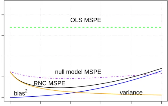
1.1 The friendship network between high school students from AddHealth study, where the edges indicate friend nominations. The nodes are colored according to the race information of students. . . 3 2.1 Mean squared prediction error EkYˆ −EYk2/n and the bias-variance trade-off of
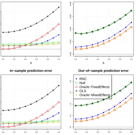
the RNC estimator (based on the upper bound (2.14) in Theorem II.6), in the setting of Example II.10 withσ= 0.5. . . 34 2.2 Linear regression with varying s andpb = 0.02. Performance is evaluated by the
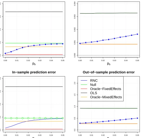
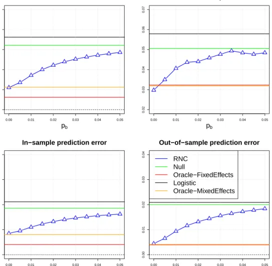
MSEs ofαandβ, and in-sample and out-of-sample mean squared prediction errors. 39 2.3 Linear regression with varying pb and s = 0.1. Performance is evaluated by the
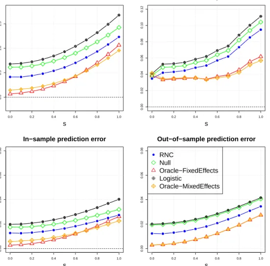
MSEs ofαandβ, and in-sample and out-of-sample mean squared prediction errors. 40 2.4 Performance logistic regression methods when varyingsand fixingpb= 0.02,
mea-sured by the MSE ofα,β, in-sample and out-of-sample mean squared probability estimation errors. . . 41 2.5 Performance of five logistic regression methods when varying pb and fixing s =
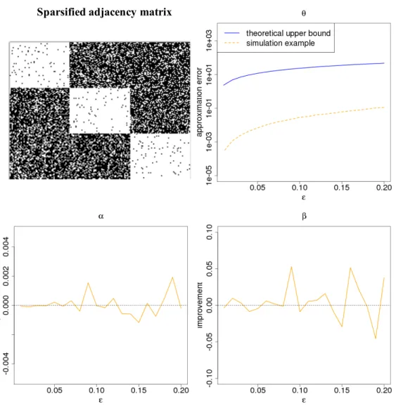
0.1, measured by the MSE of α, β, in-sample and out-of-sample mean squared probability estimation errors. . . 42 2.6 Top left: the adjacency matrix of the sparsified network for= 0.15 (white indicates
a nonzero entry, black is a zero entry); Top right: kθˆ∗−θkˆ 2and the bound (2.22); Bottom left: relative improvement of the sparsified estimatorα∗ over the original estimator ˆα, that is, 1−MSEα∗/MSEαˆ; Bottom right: relative improvement of
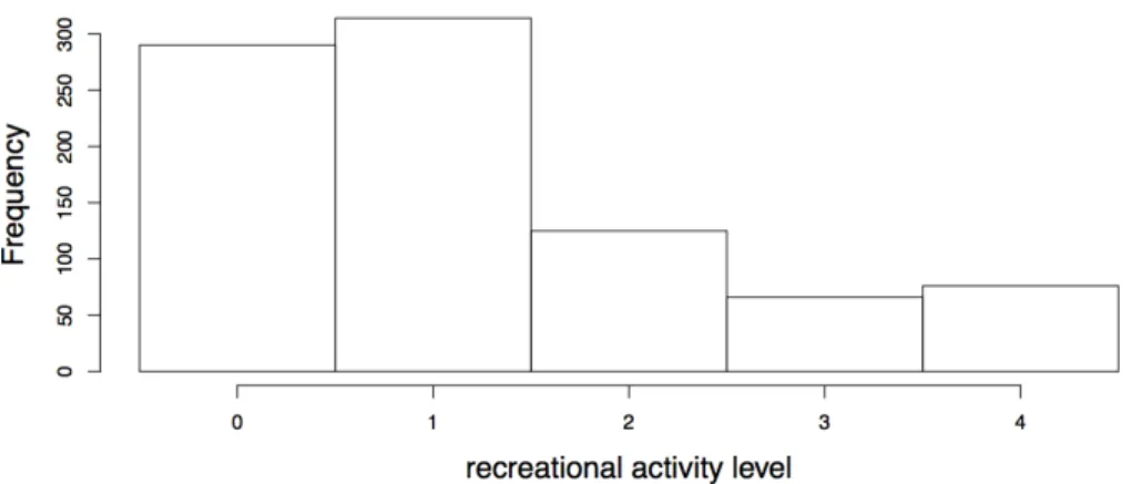
the sparsified estimatorβ∗ over the original estimator ˆβ. . . 44 2.7 Histogram of the response, recreational activity level, from the data set used in the
linear regression example. The mean recreational activity is 1.22, with standard deviation 1.23. . . 46 2.8 Age of first marijuana risk use shown on the friendship network. Node size
repre-sents the individual’s hazard, and node color reprerepre-sents the observed age of first use. . . 54 3.1 The median clustering accuracy for different fixed values of τ and for DKest and
ECV tuning. The true model is DCSBM withn= 600,K= 3, λ= 5,β= 0.2 and
t= 0. . . 88 3.2 Parameter tuning for piecewise constant graphon estimation. . . 89 3.3 The core of statistician citation network. The network has 706 nodes with node
citation count (ignoring directions) ranging from 15 to 703. The nodes sizes and colors indicate the citation counts and the nodes with larger citation counts are larger and darker. . . 91 4.1 The log-log relationship between log(P1·) and log(P1·) under the conditional NSBM.
The figures indicate an approximately linear relationship in the log scale. . . 106 4.2 Community detection accuracy of spectral methods under NSBM as a function of
t, withβ = 0.2. . . 112 4.3 Community detection accuracy of spectral methods under NSBM as a function of
β, witht= 1.5. . . 113
SCBM, as a function ofα0 with fixedβ= 0.35. . . 115 4.5 Community detection accuracy and log relative errors of estimating the probability
matrix under the conditional model, for NSBM, directed SBM, directed DCSBM, and SCBM, as a function ofβ with fixedα0= 1. . . 116 4.6 The hiring network between 87 U.S. business schools. An edge fromitoj indicates
that institution i has hired Ph.D. graduates from institution j. The node size is proportional to the receiver degree. . . 117 B.1 The rate of correctly selecting between the SBM and the DCSBM as a function of
pandN. . . 148 B.2 The rate of correctly selectingK under the true model as a function ofpand N. . 149
Table
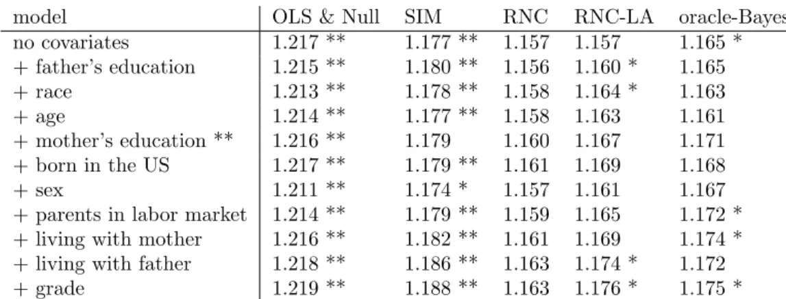
2.1 Root mean squared errors for predicting recreational activity, over 50 independent data splits into test (90 samples) and training sets. All methods are compared to RNC by a paired two-sample t-test, where ** indicatesp≤10−4 and * indicates 10−4< p < 10−2. Each row adds the variable listed to the model in the previous row, in the order determined on a separate set by forward selection with network cohesion effects included. . . 49 2.2 Average integrated AUC (iAUC) for survival prediction ROC curves for age 14-17,
over 50 random splits of the data into training and test sets. All methods are compared with RNC by a paired two-samplet-test. ** indicates p≤10−4 and * indicates 10−4< p <10−2. Each row adds the variable listed to the model in the previous row, in the order determined on a separate set by forward selection with network cohesion effects included. . . 51 2.3 Estimated covariate coefficients from regular Cox’s model and RNC for first age of
marijuana use prediction. . . 52 3.1 Ratio betweenpeand pn forn= 300,N = 3, and differentd, wherepeandpb are
the probabilities that a node withdneighbors becomes isolated in the training set in ECV and NCV, respectively. . . 74 3.2 Frequency of estimated rank values in 200 replications. . . 80 3.3 Overall model selection by ECV and NCV (fraction correct out of 200 replications).
The true model is the DCSBM. . . 82 3.4 Overall model selection by ECV and NCV (fraction correct out of 200 replications).
The true model is the SBM. . . 84 3.5 The rate of correctly estimating the number of communities (out of 200 replications)
when varying the network average degree and fixingt= 0,β = 0.2. The true model is the DCSBM. . . 85 3.6 The rate of correctly estimating the number of communities (out of 200 replications)
when varyingtand fixingλ= 40,β= 0.2. The true model is the DCSBM. . . 86 3.7 The rate of correctly estimating the number of communities (out of 200 replications)
when varyingβ and fixingλ= 40,t= 0. The true model is the DCSBM. . . 86 3.8 The rate of correctly estimating the number of communities (out of 200 replications)
for the best variant of each method. The true model is the DCSBM. . . 87 3.9 The 10 authors with largest total citation numbers (ignoring the direction) within
20 communities, as well as the community interpretations. The communities are ordered by size and authors within a community are ordered by mutual citation count. . . 92 4.1 Communities of business schools found by NSBM and their average and median
rankings from US News 2012 and Clauset et al. [2015]. Up to 15 institutions with the highestπ-ranking are shown for each community. . . 118 4.2 Estimated strengths of connections between communities. . . 119 4.3 Estimatedλi’s for Group 1 institutions. . . 120 4.4 Communities of business school institutions detected by symmetric spectral
clus-tering. . . 121
A.2 Prediction errors of five models with missing data imputation, with varying pro-portion of additional missing values. All other columns are compared with RNC by a paired two-sample t-test. ** indicates ap-value≤10−4and * indicates ap-value
∈(10−4,10−2). . . 135 A.3 Average integrated AUC (iAUC) for survival prediction ROC curves for age 14-17
with artificially increased missing values (by pm). The average is taken over 50 random splits of the data into 60 test samples and 587 training samples. All values are compared with the columns of RNC by a paired two-sample t-test. ** indicates ap-value≤10−4 and * indicates ap-value∈(10−4,10−2). . . 136 B.1 Overall block model selection correct rate of ECV and NCV in 200 replications
when binomial deviance is used as the loss function. The underlying true model is DCSBM. . . 145 B.2 Overall block model selection correct rate of ECV and NCV in 200 replications
when binomial deviance is used as the loss function. The underlying true model is SBM. . . 146 B.3 The correct rate for estimating the number of communities in 200 replications from
the best variant of each method. The underlying true model is SBM. . . 148 C.1 Communities of business school institutions detected by symmetric spectral
clus-tering. . . 159
Appendix
A. Appendix for Chapter II . . . 123
A.1 Proofs . . . 123
A.2 Complexity of solving RNC estimator by block elimination . . . 132
A.3 Coefficients of recreational activity linear models . . . 134
A.4 Sensitivity to missing data . . . 135
B. Appendix for Chapter III . . . 137
B.1 Proofs . . . 137
B.2 Additional simulation results for model selection under the block models . . 144
B.2.1 Using binomial deviance loss function for overall block model se-lection . . . 144
B.2.2 Selecting the number of communities under the SBM . . . 147
B.2.3 The impact of training proportion pand replication number N . . 147
C. Appendix for Chapter IV . . . 150
C.1 Proofs . . . 150 C.2 Community detection of business schools on the undirected hiring network . 158
Advances in data collection and social media have led to more and more network data appearing in diverse areas, such as social sciences, internet, transportation and biology. This thesis develops new principled statistical tools for network analysis, with emphasis on both appealing statistical properties and computational efficiency. Our first project focuses on building prediction models for network-linked data. Prediction algorithms typically assume the training data are independent samples, but in many modern applications samples come from individuals connected by a network. For example, in adolescent health studies of risk-taking behaviors, infor-mation on the subjects’ social network is often available and plays an important role through network cohesion, the empirically observed phenomenon of friends behav-ing similarly. Takbehav-ing cohesion into account in prediction models should allow us to improve their performance. We propose a network-based penalty on individual node effects to encourage similarity between predictions for linked nodes, and show that incorporating it into prediction leads to improvement over traditional models both theoretically and empirically when network cohesion is present. The penalty can be used with many loss-based prediction methods, such as regression, generalized lin-ear models, and Cox’s proportional hazard model. Applications to predicting levels of recreational activity and marijuana usage among teenagers from the AddHealth study based on both demographic covariates and friendship networks are discussed in detail. We show that our approach to taking friendships into account can
covariate effects.
Resampling, data splitting, and cross-validation are powerful general strategies in statistical inference, but resampling from a network remains a challenging problem. Many statistical models and methods for networks need model selection and tuning parameters, which could be done by cross-validation if we had a good method for splitting network data; however, splitting network nodes into groups requires deleting edges and destroys some of the structure. Here we propose a new network cross-validation strategy based on splitting edges rather than nodes, which avoids losing information and is applicable to a wide range of network models. We provide a theoretical justification for our method in a general setting and demonstrate how our method can be used in a number of specific model selection and parameter tuning tasks, with extensive numerical results on simulated networks demonstrating its competitiveness with task-specific methods. We also apply the method to analysis of a citation network of statisticians and obtain meaningful research communities.
Finally, we consider the problem of community detection on partially observed net-works. Communities are one important type of structure in networks and they have been widely studied. However, in practice, network data are often collected through sampling mechanisms, such as survey questionnaires, instead of direct observation. The noise and bias introduced by such sampling mechanisms can obscure the com-munity structure and invalidate the assumptions of standard comcom-munity detection methods. We propose a model to incorporate neighborhood sampling, through a model reflective of survey designs, into community detection for directed networks, since friendship networks obtained from surveys are naturally directed. We model the edge sampling probabilities as a function of both individual preferences and
the method of moments. The algorithm is computationally efficient and comes with a theoretical guarantee of consistency. We evaluate the proposed model in extensive simulation studies and applied it to a faculty hiring dataset, discovering a meaningful hierarchy of communities among US business schools.
Introduction
Advances in data collection and social media have resulted in network data being collected in many applications and at the same time, networks have been widely used to describe relationships between individuals or interactions between units of complex systems in diverse fields, including but not limited to biology, computer science, sociology and economics. There has been significant amount of work in the past two decades on network analysis and modeling which have already provided salient insights about many mechanisms such as gene regulation, friendship formu-lation and eco-system evolution [Newman, 2010]. Some networks can be directly observed, such as the social networks from online social media or road networks to describe transportation systems, while others may be inferred from other analysis, such as the protein-to-protein interaction networks or brain connectomes. Moreo-ever, the network information is sometimes collected along with more traditional covariates on each unit of analysis such as characteristics of each person, gene ex-pressions of each patient etc. [Michell and West, 1996, Pearson and Michell, 2000, Pearson and West, 2003, Harris, 2009, Ji et al., 2016]. One example of such network data is the survey data from the National Longitudinal Study of Adolescent Health (the AddHealth study) [Harris, 2009]. AddHealth was a major national longitudinal
study of students in grades 7-12 during the school year 1994-1995, after which three further follow-ups were conducted in 1996, 2001-2002, and 2007-2008. In the Wave I survey, all students in the sample completed in-school questionnaires, and a subsam-ple comsubsam-pleted a follow-up in-home interview with more detailed questions. There are questions in both the in-school survey and the in-home interview asking students to name their friends (up to 10) so friendship networks connecting students can be constructed based on this information and one can analyze the network structures to obtain insights about the friendship relation between students. In addition to the information about friends, the survey also asked hundreds of questions about various aspects of the students personal and school life, collecting information about age, gender, race, socio-economic status, health, academic achievement, etc. Figure 1.1 shows the friendship network between students in one school from the AddHealth study as well as their race information.
In general, we can represent network data in the following way: given n nodes, indexed by i = 1,2,· · · , n, we have a network connecting the n nodes, represented by an adjacency matrix A∈Rn×n such that
Aii0 =1{there is an edge from ito i0,denoted by i→i0}.
More generally, the network can be weighed, in which case we will define Aas a real matrix instead where each entry represents the edge weight or when the network is undirected, we define A to be a symmetric matrix. In some situations, we may also observe (xi, yi), i = 1,2· · · , n, where xi ∈ Rp is the covariate vector and yi is the
response variable for the node i. We can denote the matrix stacking each xi as the
ith row by X and the corresponding vector stacking all yi’s by Y. When such X
● ● ● ● ● ● ● ● ● ● ● ● ● ● ● ● ● ● ● ● ● ● ● ● ● ● ● ● ● ● ● ● ● ● ● ● ● ● ● ● ● ● ● ● ● ● ● ● ● ●● ● ● ● ● ● ● ● ● ● ● ● ● ● ● ● ● ● ● ● ● ● ● ● ● ● ● ● ● ● ● ● ● ● ● ● ● ● ● ● ● ● ● ● ● ● ● ● ● ● ● ● ● ● ● ● ● ● ● ● ● ● ● ● ● ● ● ● ● ● ● ● ● ● ● ● ● ● ● ● ●● ● ● ● ● ● ● ● ● ● ● ● ● ● ● ● ● ● ● ● ● ● ● ● ● ● ● ● ● ● ● ● ● ● ● ● ● ● ● ● ● ● ● ●● ● ● ● ● ● ● ● ● ● ● ● ● ● ● ● ● ● ● ● ● ● ● ● ● ● ● ● ● ● ● ● ● ● ● ● ● ● ● ● ● ● ● ● ● ● ● ● ● ● ● ● ● ● ● ● ● ● ● ● ● ● ● ● ● ● ● ● ● ● ● ● ● ● ● ● ●● ● ● ● ● ● ● ● ● ● ● ● ● ● ● ● ● ● ● ● ● ● ● ● ● ● ● ● ● ● ● ● ● ● ● ● ● ● ● ● ● ● ● ● ● ● ● ● ● ● ● ● ● ● ● ● ● ● ● ● ● ● ● ● ● ● ● ● ● ● ● ● ● ● ● ● ● ● ● ● ● ● ● ● ● ● ● ● ● ● ● ● ● ● ● ● ● ● ● ● ● ● ● ● ● ● ● ● ● ● ● ● ● ● ● ● ● ● ● ● ● ● ●● ● ● ● ● ● ● ● ● ● ● ● ● ● ● ● ● ● ● ● ● ● ● ● ● ● ● ● ● ● ● ● ● ● ● ● ● ● ● ● ● ● ● ● ● ● ● ● ● ● ● ● ● ● ● ● ● ● ● ● ● ● ● ● ● ● ● ● ● ● ● ● ● ● ● ● ● ● ● ● ● ● ● ● ● ● ● ● ● ● ● ● ● ● ● ● ● ● ● ● ● ● ● ● ● ● ● ● ● ● ● ● ● ● ● ● ● ● ● ● ● ● ● ● ● ● ● ● ● ● ● ● ● ● ● ● ● ● ● ● ● ● ● ● ● ● ● ● ● ● ● ● ● ● ● ● ● ● ● ● ● ● ● ● ● ● ● ● ● ● ● ● ● ● ● ● ● ● ● ● ● ● ● ● ● ● ● ● ● ● ● ● ● ● ● ● ● ● ● ● ● ● ● ● ● ● ● ● ● ●● ● ● ● ● ● ● ● ● ● ● ● ● ● ● ● ● ● ● ● ● ● ● ● ● ● ● ● ● ● ● ● ● ● ● ● ● ● ● ● ● ● ● ● ● ● ● ● ● ● ● ● ● ● ● ● ● ● ● ● ● ● ● ● ● ● ● White Black Native Asian Other
Figure 1.1: The friendship network between high school students from AddHealth study, where the edges indicate friend nominations. The nodes are colored according to the race information of students.
Many questions can be asked about analyzing a network dataset. For example, how can one build a prediction model on a network-linked data set and what are the benefits of the network information added to classical prediction setting? When the target is to understand the network structures, how can we build realistic models as well as make valid inference under a principled statistical framework? In the next a few chapters, some recent work to answer these questions will be introduced. However, we will first give a brief review for the classical setup of both predictive modeling and network analysis.
1.1 Notations
Given a positive integer n, define [n] ={1,2,· · · , n}. We will use the lower-case letters such as xto denote scalars while the bold version such asxto denote vectors, which we will treat as column vectors by default. Matrices are denoted by upper-case letters such as X. The transpose and trace of a matrix X is denoted by XT
and tr(X) respectively. For any matrix X, we use kXk to denote its spectral norm, which is the largest singular value of X and kXkF to denote its Frobenius norm,
defined by kXk2
F =
P
ijX
2
ij. We use 1n to denote the column vector ofn 1’s and In
to denote the n×n identity matrix. When it is clear in context, we may suppress the subscript.
1.2 Loss-based prediction models
Perhaps the most basic prediction model is the linear regression model. Given pairs of (xi, yi), i∈[n], where [n] := {1,2,· · · , n}, we assume
yi =α+xTi β+i.
In the model, β ∈Rp measures covariate effects,α∈
Ris the intercept and i ∈Ris
random noise, typically assumed to be i.i.d in the simple setting. The interpretation of βas covariate effects is one of the most important advantages of the linear model, giving a measure about how much change in the response one would expect due to the change of one of the covariates while fixing the rest. This interpretation admits scientific meanings and is the major target of using the model in many applications. For example, in medical studies, whenx1 is the indicator of a treatment whileyis the
health condition, the covariate effect of x1 measures whether (and to what extent)
effects of other covariates.
In spite of the simplicity, the linear modeling idea is very power in the sense that it can extended to a large class of loss-based prediction models. Given a link function φ, a generalized linear model [Nelder and Baker, 1972] is defined through the relationship
φ(Eyi) = xTi β+α
where is distribution of yi is assumed to from exponential family and the covariate
effects are still assumed in a linear form.
The linear forms are also widely used beyond generalized linear models. For instance, in survival regression problems, the Cox’s proportional hazard model [Cox, 1972] assumes the hazard for ith subject is in the form of
h0(t) exp(xTi β+α)
where h0(t) is some unspecified baseline hazard function at time t. In classification
problems, there is a family of classifiers that are assumed to have the form of
C(xi) = f(xTi β)
for some function f such that we expect to observe
yi = sign(C(xi)).
One popular method in this family of classifiers is the support vector machine (SVM) [Vapnik, 2013], which assumes f to be the identity function in its standard form.
We classify all the above models in the same family called loss-based prediction modelsdue to the common strategy available for model estimation - theM-estimation. In particular, all of the above methods can be estimated by the following problem
minimizeβ∈T L({yi,xTi β+α}ni=1)
where L is some general loss function and T is some parameter domain. For gen-eralized linear models, L is the log likelihood of the observation when one uses the maximum likelihood framework for model estimation. For the Cox’s proportional hazard model [Cox, 1972],L gives the partial likelihood function of the observations, based on which the estimation of β can be obtained. For the SVM, the L function is the hinge loss on all observations while the feasible region T is certain `2 ball of β, such that the estimation is done by
minimizeβ X i [1−yi(xTiβ+α)]+ such that kβk2 2 ≤λ
for some tuning parameter λ, according to the formulation in Hastie et al. [2009].
1.3 Random network modeling
Statistical methods for analyzing networks have received a lot of attention be-cause of its wide-ranging applications in areas such as sociology, physics, biology and medical sciences. Statistical models provide an effective way to extract structural information about the network while filtering out noisy and uninformative details thus become popular in understanding the network structures and formulation. Per-haps the simplest statistical network model is the famous Erd¨os-Renyi model [Erds and R´enyi, 1960], after which a large body of interesting models followed, including the stochastic block model (SBM) [Holland et al., 1983] and its variants such as the degree-corrected stochastic block model (DCSBM) [Karrer and Newman, 2011] or mixed membership block model (MMBM) [Airoldi et al., 2008], and the latent space model [Hoff et al., 2002], just to name a few. In this section, we introduce a
generic probabilistic framework for statistical network models - the random network modeling framework, under which a few standard models will be introduced as well. Let V = [n] denote the node set of a network, and let A be its n×n adjacency matrix. We viewAas a single random realization of independent Bernoulli variables, such that each entry of A is generated independently according to
Aii0 ∼Bernoulli(Pii0)
where P = (Pii0) ∈ [0,1]n×n. For undirected networks, we require both P and A
to be symmetric and only the upper-triangular entries of A are generated from the defined model. In this framework, the model P admits the structural information that one is interested in extracting while A is assumed to be a noisy version of P. The statistical modeling procedure is then estimating (some aspects of) P from the given noisy observation A. Many interesting statistical models have been proposed under the random network modeling framework. Below we introduce a few popular ones.
Erd¨os-Renyi model (ER) The most widely known random network model is the
Erd¨os-Renyi model [Erds and R´enyi, 1960]. Specifically, the model assumes for some
p∈[0,1]
P =p·1n1Tn = (p)n×n.
Essentially, the model assumes all of node pairs are randomly connected in a uniform way. However, the ER model is completely homogeneous and has no interesting structure. In reality, there is seldom any real world networks that can be described well by the ER model.
Stochastic block model One interesting generalization of the ER model for undi-rected networks is the stochastic block model (SBM) [Holland et al., 1983]. In the SBM, we assume each node belongs to one of the K communities. We use
c ={c1,· · · ,cn}to denote the vector of membership for all nodes, such thatci ∈[K].
Then the probability of having an edge between nodes iandj isP(Aii0 = 1) =Bc ici0
for some K×K symmetric probability matrix B. The probability matrixP can be written as P = ZBZT where Z ∈ {0,1}n×K has exactly one “1” in each row, with
Zik = 1 if node i belongs to community k. This model generalizes the ER model by
assuming the nodes are inhomogeneous across groups but remain the same within the groups.
Degree-corrected stochastic block model (DCSBM) One well-known limitation of the SBM lies in it forces equal expected degrees for all the nodes in the same com-munity, therefore ruling out “hubs” - nodes that have abnormally large number of connections compared to the rest in the population. The degree corrected stochastic block model corrects this homogenous degree problem of the SBM by associating each node i with an individual degree parameter θi. Let Θ = diag(θ1,· · · , θn). The
DCSBM then assumes P(Aii0 = 1) = θiθi0Bc
ici0. Equivalently, the P matrix is
as-sumed to be P = ΘZBZTΘ (a constraint is needed on Θ to ensure identifiability, with different authors choosing different versions; here we follow Karrer and Newman [2011] and assume P
V ci=kθi = 1, for each k∈[K]).
Random dot product graph (RDPG) The RDPG [Young and Scheinerman, 2007]
is another generalization of the SBM and one special class of latent space models. In RDPG, each node i is associated with a latent K dimensional vector Zi ∈ RK,
network only depends on K latent factors in a linear way through inner product. It has been shown that RDPG has a very good embedding properties in Euclidean space in various problems [Sussman et al., 2014, Tang et al., 2017] and its limiting behaviors can also be studied [Tang and Priebe, 2016]. More details about the model can be found in the review paper of Athreya et al. [2017].
Graphon model. Observe that random network model framework assumes that
the nodes are exchangeable. According to Aldous [1981], the probability matrix of any exchangeable random graph can be represented by
Pii0 =f(ξi, ξi0)
where function f : [0,1]×[0,1] → [0,1] is symmetric in its two arguments and is called “graphon”, whileξi, i∈[n] are independent uniform random variables on [0,1].
The representation is determined only up to a measure-preserving transformation [Diaconis and Janson, 2007]. There is a substantial literature on estimating the graphon under various assumptions [Wolfe and Olhede, 2013, Choi and Wolfe, 2014, Gao et al., 2015].
Though in this thesis, we embed our discussion of network modeling in the theme of exchangeable random network modeling framework introduced above, which in-cludes most of current random network models in statistics, there are other frame-works available, such as the one discussed by Crane and Dempsey [2015].
1.4 Outline of the thesis
The rest of the thesis is organized as follows:
Chapter II focuses on improving prediction models by incorporating network in-formationA available from the network-linked data. The high-level questions we try
to answer in Chapter II are “what are the reasonable assumptions one should as-sume for prediction models on network-linked data?” and “how can one incorporate network information wit both computationally efficiency and statistical principles?”. Specifically, we reply on one generic assumption called “network cohesion” to build prediction models, an empirically observed phenomenon of friends on social networks behaving similarly. Taking such cohesion into account in prediction models allows us to improve prediction and modeling performance. There we propose a network-based penalty on individual node effects to encourage similarity between predictions for linked nodes, and show that incorporating it into prediction leads to improvement over traditional models both theoretically and empirically when network cohesion is present. The penalty can be used with all the loss-based prediction methods intro-duced in this chapter. Applications to predicting levels of recreational activity and marijuana usage among teenagers from the AddHealth study based on both demo-graphic covariates and friendship networks are discussed in detail and show that our approach to taking friendships into account can significantly improve predictions of behavior while providing interpretable estimates of covariate effects.
Chapter III and IV focus on the problems under the random network modeling framework.
While many statistical models and methods are now available for network analysis, resampling network data remains a challenging problem. Cross-validation is a useful general tool for model selection and parameter tuning, but is not directly applicable to networks since splitting network nodes into groups requires deleting edges and destroys some of the network structure. In Chapter III, we propose a new network resampling strategy based on splitting edges rather than nodes, applicable to both cross-validation and bootstrap for a wide range of network model selection tasks. We
provide a theoretical justification for our method in a general setting and examples of how our method can be used in specific network model selection and parameter tuning tasks. Numerical results on simulated networks and on a citation network of statisticians show that this cross-validation approach works well for model selection. Chapter IV addresses a commonly encountered practical difficulty in community detection for directed networks. Communities are an important type of structure in networks and they have been widely studied. In practice, network data are often collected through sampling mechanisms, such as survey questionnaires, instead of direct observation. The noise and bias introduced by such sampling mechanisms can obscure the community structure and invalidate the assumptions of standard community detection methods. In Chapter IV, we propose a model to incorporate neighborhood sampling, through a model reflective of survey designs, into community detection for directed networks, since friendship networks obtained from surveys are naturally directed. We model the edge sampling probabilities as a function of both individual preferences and community parameters, and fit the model by a combination of spectral clustering and the method of moments. The algorithm is computationally efficient and comes with a theoretical guarantee of consistency. We evaluate the proposed model in extensive simulation studies and applied it to a faculty hiring dataset, discovering a meaningful hierarchy of communities among US business schools.
Prediction model on network-linked data
2.1 Introduction
There is a large body of work extending over decades on predicting a response variable of interest from such covariates, via linear or generalized linear models, survival analysis, classification methods, and the like, which typically assume the training samples are independent and do not extend to situations where the samples are connected by a network. There has not been much focus on developing a general statistical framework for using network data in prediction, although there are meth-ods available for specific applications [Wolf et al., 2009, Asur and Huberman, 2010, Vogelstein et al., 2013].
In the social sciences and especially in economics, on the other hand, there has been a lot of recent interest in causal inference on the relationship between a response variable and both covariates and network influences; see e.g., Shalizi and Thomas [2011] and references therein, and Manski [2013]. While in certain experimental set-tings such inference is possible [Rand et al., 2011, Choi, 2017, Phan and Airoldi, 2015], in most observational studies on networks establishing causality is substan-tially more difficult than in regular observational studies. While network cohesion (a generic term by which in this chapter we mean linked nodes acting similarly) is
a well known phenomenon observed in numerous social behavior studies [Fujimoto and Valente, 2012, Haynie, 2001, Christakis and Fowler, 2007], explaining it causally on the basis of observational data is very challenging. An excellent analysis of this problem can be found in Shalizi and Thomas [2011], showing that it is in general impossible to distinguish network cohesion resulting from homophily (nodes become connected because they act similarly) and cohesion resulting from contagion (behav-ior spreads from node to node through the links), and to separate that from the effect of node covariates themselves. However, making good predictions of node behavior is an easier task than causal inference, and is often all we need for practical purposes. Our goal in this chapter is to take advantage of the network cohesion phenomenon in order to better predict a response variable associated with the network nodes, using both node covariates and network information. While we do not attempt to make causal inferences, we do focus on interpretable models where effects of individual variables can be explicitly estimated.
Using network information in predictive models has not yet been well studied. Most classical predictive models treat the training data as independently sampled from one common population, and, unless explicitly modeled, network cohesion vi-olates virtually all assumptions that provide performance guarantees. More impor-tantly, cohesion is potentially helpful in making predictions, since it suggests pooling information from neighboring nodes. In certain specific contexts, regression with dependent observations has been studied. For example, in econometrics, following the concepts initially discussed by Manski [1993], assuming some type of an auto-regressive model on the response variables is common, such as the basic autoregres-sive model in Bramoull´e et al. [2009] and its variants including group interactions and group fixed effects [Lee, 2007]. Such models assume specific forms of different
types of network effects, namely, endogenous effects, exogenous effects and corre-lated effects, and most of this literature is focused on identifiability of such effects. In Bramoull´e et al. [2009] and Lin [2010], these ideas were applied to the AddHealth data which we discuss in detail in Section 2.5. However, these methods have mainly been used to identify social effects defined within a very specific and difficult to ver-ify model, without a focus on interpretability or good prediction performance. For instance, including neighbors’ responses as covariates in linear regression makes in-terpretation of other covariate effects more difficult, and can make the distributional assumptions difficult to satisfy. This has been done carefully in spatial statistics lit-erature, for example with the conditional autoregressive model (CAR) [Besag, 1974], but fitting these models typically requires MCMC and is very time-consuming. In addition, these methods do not extend easily beyond linear regression (for example, to generalized linear models and Cox’s proportional hazard model).
Our approach is to introduce network cohesion using penalties built using the network information, and framing the problem as loss plus penalty; for simplicity, we will present the method for regression first, and then discuss extensions to gen-eral losses. At a high level, our network penalty parallels the ideas of fusion [Land and Friedman, 1997, Tibshirani et al., 2005]. Fusion penalties generally shrink the difference between either coefficients or predictions that are expected to be similar. Fusion penalties based on a network of variables have been used in variable selection [Li and Li, 2008, 2010, Pan et al., 2010, Kim et al., 2013], but this line of work is not directly relevant here since we are interested in using the network of observa-tions, not variables. However, our approach can be viewed as a regression version of the point estimation problem discussed in Sharpnack et al. [2013] and Wang et al. [2016b]. Alternatively, it can be viewed in a Bayesian framework, as regression with
a Gaussian Markov random field prior over the network.
We show that our method gives consistent estimates of covariate effects and de-rive explicit conditions on when enforcing network cohesion in regression can be expected to perform better than ordinary least squares. In contrast to previous work, we assume no specific form for the cohesion effects and require no information about potential groups. We also derive a computationally efficient algorithm for implementing our approach, which is efficient for both sparse and dense networks, the latter with an extra sparsification step which we prove preserves the relevant network properties. To the best of our knowledge, this is the first proposal of a general prediction framework with network cohesion among the observations that is computationally feasible and can retain covariate interpretations as well as make out-of-sample predictions.
The rest of this chapter is organized as follows. In Section 2.2, we introduce our approach in the setting of linear regression. We frame it as a penalized least squares problem which has a closed-form solution, and derive its Bayesian interpretation and connection to various other models. The idea is then extended to generalized linear models. Empirically, we show that our approach outperforms prediction without networks as well as an earlier modification intended to incorporate information from neighbors. Finite sample and asymptotic properties are discussed in Section 2.3. Brief simulation results demonstrating the theoretical bounds and comparisons to benchmarks are presented in Section 2.4. A detailed analysis and discussion of cohe-sion in the AddHealth data is presented in Section 2.5, where we apply our method to predict recreational activity and marijuana usage among teenagers. All algorithms in this chapter are implemented in the R package netcoh[Li et al., 2016a], available on CRAN.
2.2 Regression with network cohesion
2.2.1 Set-up and notation
We start from reviewing the setting up of the network-linked data and notations. The data consist of n observations (x1, y1),(x2, y2),· · · ,(xn, yn), where yi ∈ R is
the response variable and xi ∈ Rp is the vector of covariates for observation i.
We write Y = (y1, y2,· · · , yn)T for the response vector, and X = (x1,x2,· · · ,xn)T
for the n × p design matrix. We treat X as fixed and assume its columns have been standardized to have mean 0 and variance 1. We also observe the network connecting the observations, G = (V, E), whereV = [n] is the node set of the graph, and E ⊂ V ×V is the edge set. We represent the graph by its adjacency matrix
A ∈ {0,1}n×n. We assume there are no loops so A
vv = 0 for all v ∈ V, and we
assume the network is undirected, i.e., Aii0 =Ai0i. The (unnormalized) Laplacian of G is given by L=D−A, whereD= diag(d1, d2,· · · , dn) is the degree matrix, with
node degree di defined bydi =
P
i0∈V Aii0. 2.2.2 Linear regression with network cohesion
Cohesion is a vague term that can be interpreted in several ways depending on whether it refers to the network itself or both the network and additional covari-ates. Cohesion defined on the network alone can be reflected in various properties, such as local density, connectivity and community structure; we refer the readers to Chapter 4 of Kolaczyk [2009] for details. In the context of prediction on networks, which is our focus, two types of cohesion are commonly discussed: homophily (also known as assortative mixing) and contagion. Homophily means nodes similar in their characteristics tend to connect, with the implication of a causal direction from sharing individual characteristics to forming a connection. In contrast, contagion
means that nodes tend to behave similarly to their neighbors, with a casual direction from having a connection to exhibiting similar characteristics. Distinguishing these two phenomena in an observational study without additional strong assumptions is not possible [Shalizi and Thomas, 2011]. Nonetheless, both of these indicate a correlation between network connections and node similarities, observed empirically by many social behavior studies [Haynie, 2001, Pearson and West, 2003, Fujimoto and Valente, 2012], and that is all we need and assume in this chapter. We use the generic term “cohesion” in order to cover both possibilities of homophily and contagion, which we do not need to distinguish.
The general cohesion penalty idea is simplest to present in the context of linear regression, so we start from this setting. Assume that
(2.1) Y =α+Xβ+
where α = (α1, α2,· · · , αn)T ∈ Rn is the vector of individual node effects, and
β = (β1, β2,· · · , βp)T ∈Rp is the vector of regression coefficients. At this stage, no
assumption on the distribution of the error is needed, but we assume E=0 and Var() = σ2I
n. For simplicity, we further assume thatn > p and XTX is invertible.
If p > nand this is not the case, the usual penalties on β, such as a lasso and ridge,
can be applied; our focus here, however, is on regularizing the individual effects, and so we will not focus on additional regularization on β that may be necessary.
Including the individual node effects α instead of a common shared intercept turns out to be key to incorporating network cohesion. In general α and β, which add up to n +p unknown parameters, cannot be estimated from n observations without additional assumptions. One well-known example of such assumptions is the simple fixed effects model (see e.g. Searle et al. [2009]), when n samples come from K known groups (typically K n), and within each group individuals share
a common intercept. Here, we regularize the problem through a network cohesion penalty on αinstead of making explicit assumptions about any structure in α.
The regression with network cohesion (RNC) estimator we propose is defined as the minimizer of the objective function
(2.2) L(α,β) = kY −Xβ−αk2+λαTLα,
where k · k is the L2 vector norm and λ > 0 is a tuning parameter. An equivalent
and more intuitive form of the penalty, which follows from a simple property of the graph Laplacian, is
(2.3) αTLα= X
(i,i0)∈E
(αi−αi0)2.
Thus, we penalize differences between individual effects of nodes connected by an edge in the network. We call this term the cohesion penalty on α. We assume that the effect of covariates X is the same across the network; as with any linear regression, two nodes with similar covariates will have similar values of xTβ, and the cohesion penalty ensures the neighboring nodes have similar individual effects α. Note that this is different from imposing network homophily (which would require nodes with similar covariates to be more likely to be connected).
The minimizer of (2.2) can be computed explicitly (if it exists) as
(2.4) θˆ = ( ˆα,βˆ) = ( ˜XTX˜ +λM)−1X˜TY. Here, X˜ = (In, X) and M = L 0n×p 0p×n 0p×p
invertible. Note that (2.5) X˜TX˜ +λM = In+λL X XT XTX ,
so it is positive definite if and only if the Schur complementIn+λL−X(XTX)−1XT =
PX⊥+λL is positive definite. From (2.3), we can see thatLis positive semi-definite
but singular since L1n = 0 and thus in principle the estimator may not be
com-putable. In Section 2.3, we will give an interpretable theoretical condition for the estimator to exist. In practice, a natural solution is to ensure numerical stability by replacing L with the regularized Laplacian L+γI, where γ is a small positive constant. Then the estimator always exists, and in fact the regularized Laplacian may better represent certain network properties, as discussed by Chaudhuri et al. [2012], Amini et al. [2013], Le et al. [2017] and others. The resulting penalty is
(2.6) X (i,i0)∈E (αi−αi0)2+γ X i α2i,
which one can also interpret as adding a small ridge penalty on α for numerical stability.
Remark II.1. The penalty (2.6) suggests a natural baseline comparison for our model which can be used to assess whether cohesion is in fact present in the data. If the graph has no edges. i.e., no information about network connections is available, the penalty (with γ = 1) reduces to a ridge penalty on the individual effects α. The parameter estimates are then obtained by minimizing
(2.7) Ln(α,β) =kY −Xβ−αk2+λkαk2 .
We call this thenull modelfor RNC, as it still incorporates individual node effects which in themselves can improve performance compared to OLS with a common
intercept. As discussed later in Section 2.2.4 and 2.2.7, this null model can also be viewed as a random effects model with i.i.d Gaussian intercepts. Comparing the fit of the null model to that of RNC can in fact provide qualitative evidence of cohesion. For linear regression, the null model can improve the fit to training data, but it gives exactly the same estimate of β as the OLS (Lemma A.3 in Appendix A), and thus cannot improve predictions on test data, since without network information individual effects on test data cannot be estimated; see more on this in Section 2.4.
Remark II.2. A possible alternative to our cohesion penalty is the network lasso penalty, P
(i,i0)∈E|αi −αi0| [Hallac et al., 2015]. However, this penalty introduces
piecewise constants on the network, a rather stronger assumption than we make about cohesion which may not be always realistic. It is also much more computa-tionally demanding, requiring a sophisticated algorithm and implementation even for moderate size networks.
Remark II.3. It is also possible to assume different but cohesive covariate effects
β for each individual, which can be implemented in exactly the same way as our idea of the individual intercepts α. As usual, there is a trade-off between including more parameters for better fit and parsimony of the model. We set β to be shared among all individual to represent the universal treatment effect, which seems to be reasonable and easy to interpret in many situations.
2.2.3 Network cohesion for general loss functions
The RNC methodology extends naturally to generalized linear models and many other regression or classification models, such as Cox’s proportional hazard model [Cox, 1972] for survival analysis, and support vector machines [Vapnik, 2013] for classification using the formulation of Wahba et al. [1999]. Here we will explicitly
write out two extensions, to generalized linear models (GLMs) and Cox’s model. For any GLM with a link function φ(EY) =Xβ+α, where α∈ Rn are the individual
effects, suppose the log-likelihood (or partial log-likelihood) function is`(α,β;X, Y). Then if the observations are linked by a network, to induce network cohesion one can fit the model by maximizing the penalized likelihood
(2.8) `(α+Xβ;Y)−λαT(L+γI)α.
When ` is concave in α and β, which is the case for exponential families, the op-timization problem can be solved via Newton-Raphson or another appropriate con-vex optimization algorithm. Note that the quadratic approximation to (2.8) is the quadratic approximation to the log-likelihood plus the penalty, and thus the problem can be efficiently solved by iteratively reweighed linear regression with network co-hesion, just like the GLM is fitted by iteratively reweighed least squares. The ridge penalty termγI helps with numerical stability and for logistic regression avoids fitted probabilities of 0 and 1 for isolated nodes, which may cause the iterative algorithm to diverge; as discussed in the previous section, adding this term to the Laplacian also improves its representation of the underlying network structure.
RNC can be similarly generalized to Cox’s proportional hazard model [Cox, 1972]. In this setting, we observe times until some event occurs, called survival times, which may be censored (unobserved) if the event has not occurred for a particular node. Cox’s model assumes the hazard function hv(y) for each individual v is
hi(y) = h0(y) exp(xTi β), i∈V,
where y is the survival time, xv is the vector of p observed covariates for individual
i, β ∈Rp is the coefficient vector and h
0 is an unspecified baseline hazard function.
effects and then encourage network cohesion. Thus we will assume the hazard for each node v is given by
(2.9) hi(y) = h0(y) exp(xTi β+αi), i∈V,
where αi is the individual effect of nodei. The appropriate loss function in terms of
the parameters θ = (α,β) is the partial log-likelihood
(2.10) `(θ;i) = X i δi xTi β+αi−log X u:yi0≥yi exp(xTi0β+αi0)
where yi is the observed survival time for node i, and δi is the censoring indicator,
which is 0 if the observation is right-censored and 1 otherwise. Note that the partial log-likelihood is invariant under a shift inαsince such a shift can always be absorbed into h0. Thus for identifiability, we require Pαi = 0. For fixed covariates xi, αi is
the individual deviation from the population average log-hazard. The sum-to-zero constraint can be automatically enforced by replacing the network Laplacian L in the network cohesion penalty with its regularized version L+γI, or equivalently adding a ridge penalty on α’s. Thus we maximize the following objective function, adding a regularized cohesion penalty to the partial log-likelihood:
`(θ)−λαT(L+γI)α.
2.2.4 A Bayesian interpretation
The RNC estimator can also be framed as a Bayesian regression model. Consider the model
Y|α,β∼ N(α+Xβ, σ2I), β ∼πβ(φ), α∼πα(Φ),
where πβ(φ) is the prior for β with hyperparameter φ, πα(Φ) is the prior for α with hyperparameter Φ, and σ2 is assumed to be known. Suppose we take π
to be the non-informative Jeffrey’s prior, reflecting lack of prior knowledge about the coefficients, and set πβ(φ) ∝1. Forα, assume a Gaussian Markov random field (GMRF) prior πα = NG(0,Φ), where Φ = Ω−1 = ζ2(L+γI)−1. Note that when
γ = 0, Ω is not invertible, and πα is an improper prior called intrinsic GMRF [Rue and Held, 2005].
If the posterior modes are used as the estimators forαandβ, then this is equiva-lent to (2.2) withλ=σ2/ζ2 and the Laplacian replaced by the regularized Laplacian
L+γI. Thus the estimator of (2.2) is the Bayes estimator with the improper intrinsic GMRF prior over the network on α. Note that this Bayesian interpretation is also valid for the generalized linear models.
2.2.5 Prediction and choosing the tuning parameter
To compute fitted values on the training data (in-sample prediction), we simply use ˆα+Xβˆ. The out-of-sample prediction task in this setting is to make predictions on a group of new subjects whose covariates as well as network connections (but not responses) become available after the model is fitted on training data. Since we have a different αv for each node v, predicted individual effects are needed for new
samples. Suppose we have a total ofntraining samples andn0 test samples, resulting in a new network with n+n0 nodes where the first n nodes are from training and the last n0 are the test nodes. Write the associated Laplacian as
L0 = L11 L12 L21 L22 ,
where L11 corresponds to the original n training samples and L22 corresponds to
the n0 test samples. Similarly write the individual effect vector as (α1,α2), where α1 = ˆαis estimated from training data, and α2 needs to be predicted.
To take advantage of cohesion, we predictα2 by minimizing the overall cohesion penalty, letting ˆ α2 = arg min α2 ( ˆα,α2)TL0( ˆα,α2) . This gives ˆ α2 =−L−221L21αˆ.
This corresponds to a supervised prediction setting, our focus in this chapter, which assumes only the training data are available at the time of fitting. Our method can also be used in a semi-supervised setting, where the entire network is available at the time of training. In this case, the cohesion penalty at the fitting stage can include all the individual effects for all data points and the entire network so α1 and α2 are jointly optimized simultaneously.
The tuning parameter λ can be selected by cross-validation. Randomly splitting or sampling from a network is not straightforward; however, we found that the usual “naive” cross-validation finds very good tuning parameters for our method, perhaps because it is fundamentally a regression problem and we are not attempting to make any inferences about the structure of the network. We tune using regular 10-fold cross-validation, randomly splitting the samples into 10 folds, leaving each fold out in turn, and training the model using the remaining nine folds and the corresponding induced subnetwork. The cross-validation error is computed as the average of the prediction errors on the fold that was left out, and the tuning parameter is picked to minimize the cross-validation error.
2.2.6 An efficient computation strategy
Computing the estimator (2.4) involves solving a (n+p)×(n+p) linear system so a naive implementation would require O((n+p)3) operations. For GLMs, such
a system has to be solved in each Newton step. This computational burden can be reduced significantly by taking advantage of the fact that most networks in practice have sparse adjacency matrices as well as sparse Laplacians, which allows for using block elimination. A general description of this strategy can be found in many standard texts (see e.g. Boyd and Vandenberghe [2004], Ch. 4). Here we give the details in our setting.
The linear system we need to solve is
( ˜XTX˜ +λM)a =b.
From (2.5), we can rewrite this system with the following block structure:
I+λL X XT XTX a1 a2 = b1 b2 .
The top row gives
(I+λL)a1 = (b1−Xa2)
and substituting this into the bottom row, we have
(XTX−XT(I+λL)−1X)a2 =b2−XT(I+λL)−1b1.
Note that I +λL is a symmetric diagonal dominant (SDD) matrix, and is sparse most of the time in practice, so (I +λL)−1b
1 and (I +λL)−1X can be efficiently
computed [Koutis et al., 2010, Cohen et al., 2014]. The cost of this step is roughly
O(p(n+ 2|E|)(logn)1/2), where |E| is the number of edges in the network and c is
some absolute constant. The cost of the remaining computations is dominated by the cost of inverting the p×pmatrix XTX−XT(I+λL)−1X, which is of the same
order as the cost of solving a standard least squares problem.
When A and L are dense matrices, with|E|=O(n2), the strategy above has the
we do not gain anything from block elimination unlessL is sparse. However, we can first apply a graph sparsification algorithm to A and use the sparsified A∗ as input for RNC. For instance, the algorithm of Spielman and Teng [2011] can find A∗ with
O(−2nlogn) edges at the cost of O(|E|log2n) operations such that its sparsified Laplacian L∗ satisfies
(1−)LL∗ (1 +)L,
for a given constant > 0. After this sparsification step, the complexity of solving the linear system reduces to toO(pnlogcn) forc≤3. In Section 2.3, we will provide theoretical guarantees for the accuracy of the RNC estimator based on L∗ compared to that based on L.
When the number of edges is on the order of O(n2), the sparsification step itself
has complexity of O(n2logcn), which is not necessarily cheaper than directly solving
the original dense linear system using the SDD property. However, the advantage of sparsification becomes obvious when one has to iteratively solve the linear system for the GLM or Cox’s model, and/or compute a solution path for a sequence of λ
values. In such situations, sparsificaiton only has to be done once and the average complexity of solving the linear system can be close to O(nlogcn) for the whole estimation procedure. Details of complexity calculations for the RNC are given in Appendix A.2; a more comprehensive discussion of the computational trade-off of sparsification can be found in Sadhanala et al. [2016].
2.2.7 Connection to other models
Fixed group effects models The fixed effects regression model with subjects divided into groups is a special case of RNC. If the graph G represents the groups as cliques (everyone within the same group is connected), there are no connections between
groups, and we letλ→ ∞, then all nodes in one group will share a common intercept.
Mixed effects models. A mixed model, like ours, has individual effects viewed as random (α) and fixed covariate effects (β), but no network effects. Our null model is a standard mixed model. The Bayesian interpretation of our method suggests we are inducing correlations between the random effects, α∼ NG(0,Φ). The estimator (2.4) is then the mixed model equation in Henderson [1953] for estimating fixed effects and predicting random effects simultaneously (see Searle et al. [2009]). However, the framework of mixed models requires stronger assumptions on the form of variance components. Moreover, (generalized) mixed models are not designed for predictions conceptually, and we will show in the simulation study as well as theoretically in Lemma A.3 in Appendix A that the null model is not able to improve on out-of-sample predictions.
Spatial models In spatial statistics, data points are typically indexed by their locations. A weight matrix A can be computed as a function of distance between locations and can be used as a weighted analogue of our network adjacency ma-trix. This leads to natural connections between RNC and methods used in spatial statistics. In particular, ignoring the covariates X, RNC reduces to the Laplacian smoothing point estimation procedure in Sharpnack et al. [2013] and Wang et al. [2016b], which is equivalent to krigging in spatial statistics [Cressie, 1990]. It has been shown that a class of semi-supervised learning methods based on Laplacian smoothing can be viewed as “graph krigging” [Xu et al., 2010] . From this perspec-tive, RNC can be viewed as a generalization of graph krigging of Xu et al. [2010] to incorporate covariates and general loss functions. With covariates X included, the Bayesian interpretation of RNC assumes the same Gaussian Markov random
field distribution for α as the conditional autoregressive model (CAR) [Besag, 1974] and its GLM generalization (Chapter 9 of Waller and Gotway [2004]) assume for errors in spatial regression. However, ζ2 and σ2 in our Bayesian interpretation are treated as parameters in the CAR, while λ=σ2/ζ2 is treated as a tuning parameter in RNC. Further, the CAR model is fitted either by maximum likelihood involving computationally expensive integration steps, or by posterior inference via Markov chain Monte Carlo after assuming a full Bayesian model with additional priors on β
and ζ2, etc. Both ways require much heavier computations than RNC, especially for GLM where the Gaussian Markov random field is no longer the conjugate prior. More importantly, CAR models cannot be applied to general loss functions that are not a well-defined likelihood, for example, for Cox’s model and SVM. Also, CAR models suffer from conceptual difficulties in making out-of-sample predictions [Waller and Gotway, 2004]. In contrast, RNC provides a universal strategy under general loss functions and comes with a natural out-of-sample predictor, discussed in Section 2.2.5.
Manifold embeddings Our Laplacian-based penalty has connections to the large literature on manifold embeddings and semi-supervised learning. The general task of manifold embeddings is to embed data points, typically observed in some high-dimensional space equipped with a potentially non-Euclidean similarity measure, into a low-dimensional Euclidean space, while preserving dissimilarity between the points as much as possible. Finding the “right” embedding space is expected to help with downstream analysis tasks, such as visualization [Tenenbaum et al., 2000] or clustering [Shi and Malik, 2000]. Perhaps the algorithm most closely related to ours is Laplacian Eigenmaps [Belkin and Niyogi, 2003], which proposed using k
eigenvec-tors of the constructed graph Laplacian L corresponding to the smallest eigenvalues as the Euclidean embedding of the graph in order to obtain a low-dimensional rep-resentation of the data, and its kernel version with a regularization penalty [Belkin et al., 2006]. There are multiple semi-supervised learning approaches to prediction on manifolds, where it is assumed that all the similarities (corresponding to the network in our case) are observed but only some of the data points are labelled [Zhou et al., 2004, 2005]. Later out-of-sample extensions [Bengio et al., 2004, Cai et al., 2007, Vural and Guillemot, 2016] were developed by assuming the embedding coordinates take certain specific forms as functions of the original data points, and in general the manifold literature relies on an underlying Euclidean space where distance and smoothness are well defined, an assumption we do not make.
Supervised manifold embeddings have also been proposed when class labels are available in training data, including for the Laplacian Eigenmaps [Yang et al., 2011, Raducanu and Dornaika, 2012, Vural and Guillemot, 2016]. The basic idea is to learn a low-dimensional embedding of the data that also corresponds to a good separation of classes, and then use the coordinates in this embedding as predictors instead of the original variables. For general response variables instead of class labels, there is no supervised variant of Laplacian Eigenmaps as far as we are aware. More importantly, the embedding coordinates are typically complicated implicit functions of all the variables, and their coefficients cannot be interpreted in any meaningful way. Our method, on the other hand, has the original variables as predictors in the model (and nothing else), and thus their regression coefficients are readily interpretable.
2.3 Theoretical properties of the RNC estimator
Recall the RNC estimator is given by
(2.11) θˆ = ( ˜XTX˜ +λM)−1X˜TY, where M = L 0 0 0 .
We continue to assume that X has centered columns and full column rank. Intu-itively, we expect the network cohesion effect to improve prediction only when the network provides “new” information that is not already contained in the predictors
X. We formalize this intuition in the following assumption:
Assumption II.4. For any u6= 0 in the column space of X, uTLu>0.
This natural and fairly mild assumption is enough to ensure the existence of the RNC estimator. Write col(X) for the linear space spanned by columns of X and col(X)⊥ for its orthogonal complement. Then the projection matrix onto col(X)⊥ is PX⊥ = In−PX, where PX = X(XTX)−1XT. Write λmin(M) for the minimum
eigenvalue of any matrix M. Then we have the following lemma:
Proposition II.5. Whenever λ >0, we have 0≤ ν =λmin(PX⊥ +λL)≤1. Under
Assumption II.4 the RNC estimator (2.11) exists.
Lemma II.5 in the Appendix shows that when the network is connected and X is centered, the RNC estimator always exists since in a connected graph, L has rank
n−1, and an eigenvector 1.
(2.11) satisfies MSE( ˆα) ≤ λ 2 ν2kLαk 2 +n νσ 2 , (2.12) MSE( ˆβ) ≤ λ 2 ν2µkLαk 2+σ2(1 ν + 1)tr((X TX)−1), (2.13) EkYˆ −EYk2 ≤ λ 2 ν kLαk 2 +σ2kS λk2F, (2.14)
where the minimum eigenvalue of XTX is denoted by µ and kS
λkF is the Frobenius norm of the shrinkage matrixSλ = ˜X( ˜XTX˜+λL)−1X˜T. In particular, whenkLαk=
0, and therefore α is constant over each connected component of the network, RNC is unbiased.
The proof is given in the Appendix where the expressions for exact errors are also available. Theorem II.6 applies to any fixed n. The asymptotic results as the size of the network n grows are presented next in Theorem II.7. We add the subscriptn to previously defined quantities to emphasize the asymptotic nature of this result.
Theorem II.7. If Assumption II.4 holds, µn = O(n), kLnαnk2 = o(nc) for some constant c < 1, and there exists a sequence of λn and a constant ρ > 0 such that
lim infnνn > ρ, then
MSE( ˆβ)≤O(λ2nn−(1−c)) +O(n−1).
Therefore if λ2n=o(n1−c), βˆ is anL2-consistent estimator of β.
Remark II.8. Note that the quantityLαappearing in the assumptions is the gradient of the cohesion penalty with respect toα,∇ααTLα= 2Lα. We callLαthe cohesion gradient. In physics, cohesion gradient is used to measure heat diffusion on graphs when α is a heat function:
(Lα)i =|ne(i)| αi− P i0∈ne(i)αi0 |ne(i)| ! .
where ne(i) is the set of neighbors of i defined by the graph. Thus kLαk represents the difference between nodes’ individual effects and the average of their neighbors’ effects. The condition of Theorem II.7 requires that the norm of the vectorLα∈Rn
grows slower thanO(√n). This condition is satisfied by a large set of n−dimensional vectors defined on many networks; the following proposition gives an example.
Proposition II.9. Assume the network is a √n ×√n lattice. Then kLαk2 ≤ nc as long as α is in the subspace spanned by k smallest eigenvalues of L for some
k ≤Cn1+c2 , where C and c are some constants and c <1.
It is instructive to compare the MSE of our estimator with the MSE of the ordinary least squares (OLS) estimator, as well as the null model (which is what our estimator gives when the network has no edges). For OLS, we have
ˆ
βOLS = (XTX)−1XTY, αˆOLS = ¯y1,
wher