Transcoding Live Adaptive Video Streams
at a Massive Scale in the Cloud
Ramon Aparicio-Pardo
Telecom Bretagne, France
Karine Pires
Telecom Bretagne, France
Alberto Blanc
Telecom Bretagne, France Telecom Bretagne, France
Gwendal Simon
ABSTRACT
More and more users are watching online videos produced by non-professional sources (e.g., gamers, teachers of online courses, witnesses of public events) by using an increasingly diverse set of devices to access the videos (e.g., smartphones, tablets, HDTV). Live streaming service providerscan combine adaptive streaming technologies and cloud computing to satisfy this demand. In this paper, we study the problem of preparing live video streams for delivery using cloud computing infrastructure, e.g., how many representations to use and the corresponding parameters (resolution and bit-rate). We present an integer linear program (ILP) to maximize the average user quality of experience (QoE) and a heuristic algorithm that can scale to large number of videos and users. We also introduce two new datasets: one characterizing a popular live streaming provider (Twitch) and another characterizing the computing resources needed to transcode a video. They are used to set up realistic test scenarios. We compare the performance of the optimal ILP solution with current industry standards, showing that the latter are sub-optimal. The solution of the ILP also shows the importance of the type of video on the optimal streaming preparation. By taking advantage of this, the proposed heuristic can efficiently satisfy a time varying demand with an almost constant amount of computing resources.
Categories and Subject Descriptors
H.5.1 [Information Interfaces and Presentation]: Multimedia Information Systems—Video
General Terms
Algorithm, Design, Measurement
Keywords
Live streaming, cloud-computing, video encoding
Permission to make digital or hard copies of all or part of this work for personal or classroom use is granted without fee provided that copies are not made or distributed for profit or commercial advantage and that copies bear this notice and the full citation on the first page. To copy otherwise, to republish, to post on servers or to redistribute to lists, requires prior specific permission and/or a fee. Request permissions from [email protected].
MMSys ’15,March 18 - 20 2015, Portland, OR, USA Copyright 2015 ACM 978-1-4503-3351-1/15/03 ...$15.00 http://dx.doi.org/10.1145/2713168.2713177
1.
INTRODUCTION
The management of live video services is a complex task due to the demand for specialized resources and to real-time constraints. To guarantee the quality of experience (QoE) for end-users, live streaming service
providers (e.g., TV operators and multimedia
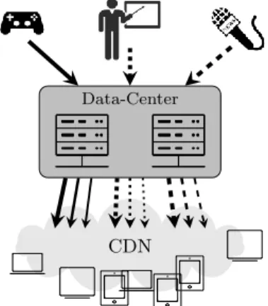
broadcasters) have traditionally relied on private data-centers (with dedicated hardware) and private networks. The widespread availability of cloud computing platforms, with ever decreasing prices, has changed the landscape [17]. Significant economies of scale can be obtained by using standard hardware, Virtual Machine (VM), and shared resources in large data-centers. As illustrated in Figure 1, live streaming providers use these services in combination with widely available content delivery network (CDN) to build an elastic and scalable platform that can adapt itself to the dynamics of viewer demand. The only condition is to be able to use the standardized cloud computing platforms to prepare the video for delivery.
The emergence of cloud computing platforms has enabled some new trends, including: (i) the adoption of adaptive bit-rate (ABR) streaming technologies to address the heterogeneity of end-users. ABR streaming requires encoding multiple video representations, and thus increases the demand for hardware resources. Modern cloud computing platforms can meet this demand. And (ii) the growing diversity of live video streams to deliver. The popularity of services like Twitch [1] illustrates the emergence of new forms of live streaming services, where the video stream to be delivered comes from non-professional sources (e.g., gamers, teachers of online
Data-Center
CDN
courses, witnesses of public events). Instead of a few high-quality well-defined video streams, live streaming providers have now to deal with many low-quality unreliable video streams.
In comparison to the significance of the shift, relatively few academic studies have been published. The scientific literature contains papers related to ABR streaming into CDN (e.g., [2, 14]). However, to the best of our knowledge, the preparation of the streams into data-centers has not been addressed by the scientific community. The preparation of a given video channel includes deciding the number of representations to encode, setting the encoder parameters, allocating the transcoding jobs to machines, and transcoding each raw video stream into multiple video representations.
Existing works address some of these problems individually. For instance, some papers [7, 9, 11–13] present algorithms to schedule transcoding jobs on a group of computers, typically in order to maximize CPU utilization [7, 11] or to minimize the finishing time [12, 13]. Other researchers have analyzed the performance of video encoding and the relationship between power, rate and distortion [8, 21, 25] using analytical models and empirical studies. In each case the encoding parameters (i.e., resolution and rate) are input parameters of these algorithms, and are assumed to be known. Yet, they can have a significant impact on the QoE and on the total bandwidth used, as discussed in [22].
Even though solutions have already been proposed for these subproblems, it is non-trivial to combine them to form a single solution and there is no guarantee that a combination of optimal solutions of each subproblem is an optimal and feasible solution of the global problem. For example, selecting the available representations (resolution and bit-rate) without considering the available computing resources is likely to lead to unfeasible solutions.
In this paper we are interested in maximizing the average user QoE by selecting the optimal encoding parameters under given computing and CDN capacity constraints. More specifically, we make three contributions: 1. We provide three datasets to help the community study the problem of preparing ABR video in data-centers. The first dataset is based on a measurement campaign we have conducted on Twitch between January and April 2014. The second dataset, based on [4], gives bandwidth measurements on real clients downloading ABR streams. The third dataset is the result of a large number of transcoding operations that we have done on a standard server, which is typical of commoditized data-center hardware. Thanks to this dataset, it is possible to determine the computing resources needed to transcode a video and the QoE of the output video. 2. We formulate an optimization problem for the
management of a data-center dealing with a large number of live video streams to prepare for delivery (section 5). Our goal is to maximize the QoE for the end-users subject to the number of available machines in the data-center. With this problem, we highlight the complex interplay between the popularity of channels, the required computing resources for video transcoding, and the QoE of
end-users. We formulate this problem as an integer linear program (ILP). We then use a generic solver to compare the performances of standard stream preparation strategies (where all the channels use the same encoding parameters for the transcoding operation) to the optimal. Our results highlight the gap between the standard preparation strategies and the optimal solution.
3. We propose a heuristic algorithm for the preparation of live ABR video streams (section 6). This algorithm can decide on-the-fly the encoding parameters. Our results (section 6) show that our proposal significantly improves the QoE of the end-users while using almost constant computing resources even in the presence of a time varying demand.
2.
RELATED WORKS
Cloud-based transcoding has been the subject of several papers. Most of these works [7, 9, 11–13] take advantage of the fact that some modern video compression techniques divide the video stream into non-overlapping Group of Pictures (GOPs) that can be treated independently of each other. The encoding time of each GOP depends on its duration and on the complexity of the corresponding scene. The algorithms exploit this fact to increase the utilization of each computing node at the expense of an increased complexity, including the time and resources needed to split the input video into appropriately sized GOP.
One downside of these solutions is that they need to know the transcoding time of each GOP in order to assign it to the most suitable computing node. Some authors [7, 11] propose fairly complicated systems to estimate the encoding time of each GOP based on real-time measurements, while others [9, 12, 13] assume that this information is directly available, for instance [9] by profiling the encoding of a few representative videos of different types, similarly to what we have done (see section 3.2). Another downside of a GOP-based solution is that the encoding of each GOP can be completed out of order and then need to be reordered before being delivered to the users. This out-of-order problem is especially important when dealing with live content that requires real-time constraints. Only Huang et al. [9] explicitly consider real-time constraints in a GOP-based system.
Lao et al. [12] and Lin et al. [13] deal only with batches of videos to transcode and present different scheduling algorithms to minimize the overall encoding time.
Zhi et al. [23] propose to leverage underused CDN computing resources to jointly transcode and deliver videos by having CDN servers transcode and store the most popular video segments. Such a solution can offer significant gains, especially for non-live popular streams, but it requires the cooperation of the CDN, which is not always owned and operated by the cloud provider.
Cheng et al. [6] present a framework for real-time cloud-based video transcoding in the context of mobile video conferencing. Depending on the number of participants and their locations, every video conference corresponds to one or more transcoding jobs, each one located in a potentially different data center. They use a simple linear model to estimate the resources needed by each transcoding job; if the currently running VMs have
enough spare capacity to handle the new job, they use them, otherwise they start new VMs, without a constraint on the total number of VMs used. They assume alinear relationship between the video encoding rate and CPU usage, based on some measurements, for which no details are given. As shown in section 3.2, this is not consistent with our experiments usingffmpegtoencodeH.264 videos. The literature on video encoding is vast. A few papers have studied the relationship between power consumption, rate and distortion (often abbreviated as P-R-D). The first paper to investigate the P-R-D model by He et al. [8] contains a detailed analysis and corresponding model of the video encoding process. The authors use this model to define an algorithm that, given rate and power constraints, minimizes the distortion of the compressed video. Su et al. [21] use a different definition for the distortion and propose a different algorithm to solve the same optimization problem. These works deal witha single video flow and take the rate as an input parameter, they do not address how to chose its value.
Yang et al. [25] present the results of an empirical study based on the H.264 Scalable Video Coding (SVC) reference software JSVM-9.19 [18]. While non-SVC H.264 can be considered as a special case consisting of only one layer, the authors emphasize the results related to the SVC part. Since the raw data is not publicly available, and since the figures in the paper do not correspond to the inputs we need, we run similar experiments leading to the dataset presented in section 3.2.
3.
PROBLEM DEFINITION BY DATASETS
In this Section, we present the three datasets used throughout the paper. They will help us to introduce the parameters influencing the stream preparation. The three datasets cover the chain of involved (directly or indirectly) actors: broadcasters, live service provider, and viewers.
3.1
The Broadcasters
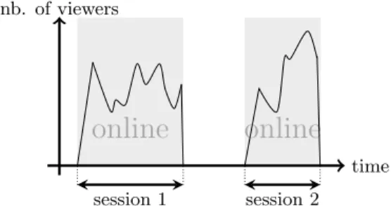
We will interchangeably use the terms channel and broadcaster to indicate the people using the live streaming system to deliver a video. At any given time, a channel can be either online, when the broadcaster emits the video stream, or offline when the broadcaster is disconnected. Each online period is called asession. During a session, a broadcaster captures a video, encodes it, and uploads it to the service provider. We say that this video stream is the source or the raw video stream. The service provider is then in charge of transcoding this video into one or multiple video representations, and of delivering these representations to the viewers, or end-users. The number of viewers watching a session can change over time. Figure 2 shows the evolution of the popularity of a given channel over time, this channel containing two sessions.
Today’s channels in cloud-based live streaming services are mostly “non-professional.” We focus here on the thousands of broadcasters who use live streaming services such as ustream,1 livestream,2 twitch,3 and dailymotion4 to broadcast live an event that they are capturing from 1http://www.ustream.tv/ 2 http://new.livestream.com/ 3http://www.twitch.tv/ 4 https://www.dmcloud.net/features/live-streaming
online
online
nb. of viewers time session 1 session 2Figure 2: A life in a channel
their connected video device (e.g., camera, smartphone, and game console). As opposed to the traditional TV providers and the content owners from the entertainment industry, these broadcasters usually do not emit ultra-HD video streams (2160p also known as4k) and they tolerate a short lag in the delivery. However, these broadcasters are less reliable. First, a channel can switch from offline to online and vice versa at any time. Second, the emitted streams have various bit-rates and resolutions, as well as various encoding parameters. Third, the broadcasters do not give much information about their video streams.
In this paper, we use a dataset based on Twitch, a popular live streaming systems. Twitch provides an Application Programming Interface (API) that allows anybody to fetch information. We used a set of synchronized computers to obtain a global state every five minutes (in compliance with API restrictions) between January, 6th and April, 6th 2014. We fetched information about the total number of viewers, the total number of concurrent online channels, the number of viewers per session, and some channel metadata. We then filtered the broadcasters having abnormal behavior (no viewer or online for less than five minutes during the last three months). The dataset is publicly available.5 We summarize the main statistics in Table 1.
Data Statistics
total nb. of channels 1,536,492
total nb. of sessions 6,242,609
“online less than 5 min. overall” channels 25%
“no viewer” channels 11%
filtered nb. of channels 1,068,138 (69%) filtered nb. of sessions 5,221,208 (83%)
Table 1: The Twitch dataset
Figure 3 shows the average number of concurrent online channels, which is a useful metric to estimate the computing power needed and thus the data-center dimensions. Between 4,000 and 8,000 concurrent sessions always require data-center processing.
To illustrate the diversity of the raw videos, Figure 4 shows the cumulative density function (CDF) of the bit-rates of sessions for the three most popular resolutions. The key observation is the wide range of the bit-rates, even for a given resolution. For example, the bit-rates of 360p sources range from 200 kbps to more than 3 Mbps.
5
0 10 20 30 40 50 60 70 80 90 0 2 000 4 000 6 000 8 000 10 000 Days N b. of o nline chan
nels max min
Figure 3: Number of concurrent sessions in Twitch (min and max per day)
100 1 000 10 000 0 0.2 0.4 0.6 0.8 1 Video bit-rate (kbps) CD F of the session s 1080p 720p 360p
Figure 4: CDF of the session source bit-rates
3.2
The Live Streaming Service Provider
One of the missions of the live streaming service is to transform the raw video into a multimedia object that can be delivered to a large number of users. We call preparationthis phase. In this paper, we focus on the task of transcoding the raw video stream into a set of ABR video streams for delivery, and we neglect other tasks such as content sanity check and the implementation of the digital right management policy. For each session, our goal is twofold: (i) to define the set of video representations to be transcoded, which supposes to decide the number of representations, and, for each representation, the bit-rate and the resolution; and, (ii) to assign the transcodingjobs to the data-center machines.A key information for our study is the amount of central processing unit (CPU) cycles that are required to transcode one raw video into a video stream in a different format. This quantity depends on various parameters, but mostly on (i) the bit-rate and the resolution of the source, (ii) the type of the source, and (iii) the bit-rate and the resolution of the target video stream. To obtain a realistic estimate, we have performed a set of transcoding operations from multiple types of sources encoded at different resolutions and rates to a wide range of target resolutions and rates. For each one of the transcoding operations, we have estimated the QoE of the transcoded video, and measured the CPU cycles required to perform it. This dataset as well is publicly available.6
Source Types. We consider four types of video content, corresponding to four test sequences available at [24]. Each of these four test sequences corresponds to a representative video type as given in Table 2.
6
http://dash.ipv6.enstb.fr/dataset/transcoding/
Video Type Video Name
Documentary Aspen, Snow Mountain
Sport Touchdown Pass, Rush Field Cuts Cartoon Big Buck Bunny, Sintel Trailer Video Old Town Cross
Table 2: Test videos and corresponding type.
Source Encoding. In current live streaming systems, the encoding of the source is done at the broadcaster side. As shown in Figure 4, the raw video that is emitted by the broadcaster can be encoded with different parameters. Based on our analysis of the Twitch dataset, we consider only four resolutions, from 224p to 1080p, and we let the analysis of 4kraw videos for future works. We also restrict the video bit-rates to be in ranges covering 90% of the sources that we observe in the Twitch dataset. See Table 6 in the Appendix for more details.
Target Videos. The format of the target videos depends on the source video. For each input video we consider all the resolutions that are smaller than or equal to the input video and for each resolution we consider all the rates that are smaller or equal to the rate of the input video (see Table 6 in the Appendix for more details).
Transcoding. We perform the transcoding on a standard server, similar to what can be found in most public data-centers. The debate about whether graphics processing unit (GPU) can be used in a public cloud is still acute today. Those who do not believe in a wide availability of GPU in the cloud emphasize the poor performance of standard virtualization tools on GPU [19] and the preferences of the main cloud providers for low-end servers (the so-called wimpy servers) in data-centers [3]. On the other hand, new middleware have been developed to improve GPU sharing and VM-GPU matching in data-centers [16], so it may be possible to envision a wider deployment of GPU in a near future. Nevertheless, in this paper, we stick to a conservative position, which is the one adopted by today’s live streaming service providers, and we consider only the availability of CPU in the servers.
As for the physical aspect of the CPU cycles measurements, we consider that the virtualization has no impact on the performances,i.e. a transcoder running in a VM on a shared physical machine is as fast as if it ran directly on the physical machine. The server that we used is an Intel Xeon CPU E5640 at 2.67GHz with 24 GB of RAM using Linux 3.2 with Ubuntu 12.04.
Figure 5 shows the experimental results for all the target videos generated from a source of type “movie,” 1080p resolution and encoded at 2,750 kbps. The empirical CPU cycles measurements are depicted as marks. Section A.2 in the Appendix, gives more details on how these curves have been generated. Overall, 588 curves similar to these ones were prepared to cover the 12,168 transcoding operations. For the sake of brevity, we show only these four. The interested reader can consult the full set of curves in the publicly available dataset, as mentioned above.
Estimating QoE. We evaluate the QoE by means of the Peak Signal to Noise Ratio (PSNR) score [20], which is a full-reference metric commonly used due to its simplicity. We
apply the PSNR filter7 provided byffmpegin two different cases illustrated in Figure 7.
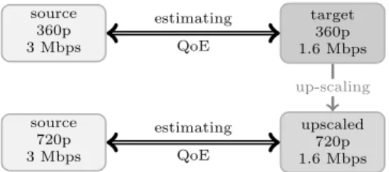
The first case, depicted on top of Figure 7, corresponds to the scenario where a target (transcoded) video at a given spatial resolution is watched on a display of the same size. The PSNR filter compares the target video against a reference video. The reference is the source encoded at the same resolution as the target but with the largest encoding bit-rate considered in this study (3,000 kbps). We repeat this measurement as many times as target videos, i.e., 12,168 times. As in the case of the live-transcoding CPU curves, we only depict in Figure 6 the PSNR curves corresponding to one example. We provide the remaining set of curves in the public site hosting the dataset.
The second scenario, shown on bottom of the Figure 7, refers to the situation when a target (transcoded) video at a given resolution need to be upscaled to be watched on a display with a higher size. This up-scaling introduces a penalty on the final QoE for the viewer. To estimate these penalties, we carry out a new battery of transcoding operations, using the sameffmpegcommand as before, but the input and output video are the target and the upscaled video, respectively. The upscaled video is compared against a reference with an encoding rate of 3,000 kbps but with the same resolution as the upscaled target. The penalty, using the example of up-scaling from 360p to 720p in Figure 7, can simply be computed by subtracting from the PSNR measure on top of the Figure the PSNR measurement on the bottom. In Figure 8, we depict the up-scaling penalties for a 224p source of type movie.
500 1000 1500 2000 2500 0.6 0.8 1 1.2 1.4 1.6
Target rate (in kbps)
CP U (i n GH z ) 224p 360p 720p 1080p
Figure 5: Transcoding CPU curves. Source: 1080p, 2,750 kbps, typemovie. Target resolutions in the legend.
500 1000 1500 2000 2500 30 32 34 36 38 40
Target rate (in kbps)
PS N R (i n d B ) 1080p 720p 360p 224p
Figure 6: Transcoding QoE curves. Source: 1080p, 2,750 kbps, typemovie. Target resolutions in the legend.
7 https://www.ffmpeg.org/ffmpeg-filters.html#psnr source 360p 3 Mbps source 720p 3 Mbps target 360p 1.6 Mbps upscaled 720p 1.6 Mbps estimating QoE estimating QoE up-scaling
Figure 7: Estimating the QoE for a target video. On top, a video at 360p and 1.6 Mbps. On the bottom, the same video upscaled to be watched on a 720p display.
500 1000 1500 2000 2500 3000 −12 −10 −8 −6 −4 −2 Rate (in kbps) PS N R (i n d B ) 360p 720p 1080p
Figure 8: Up-scaling penalties curves. Sources: rate in x-axis, 224p, type movie. Target resolutions in the legend. Target rates equal to source rates
3.3
The Viewers
Finally, we need a dataset that captures the characteristics of a real population of viewers, and in particular its heterogeneity.
This dataset comes from [4]. Since the Twitch API does not provide any information about the viewers (neither their geographic positions, nor the devices and the network connections), we need real data to set the download rates for the population of viewers. The dataset presented in [4] gives multiple measurements over a large number of 30s-long DASH sessions from thousands of geographically distributed IP addresses. From their measurements, we infer the download rate of each IP address for every chunk of the session and thus obtain 500,000 samples of realistic download rates. After filtering this set to remove outliers, we randomly associate one download rate to one of the viewers watching a channel from the Twitch dataset snapshot.
4.
CURRENT INDUSTRIAL STRATEGIES
Today’s live service provider have to implement a strategy for stream preparation. To the best of our knowledge, no provider has yet implemented an optimal strategy. Typically one of the following two options is implemented. In the first one, used by Twitch, ABR streaming is only offered to some premium broadcasters. That is, only a small subset of channels is transcoded into multiple representations. For the other broadcasters, the raw video is forwarded to the viewers without transcoding. The problem of this solution is that many viewers of standard broadcasters cannot watch the stream because their downloading rate is too low. This problem has been recently discussed in [15].
The second option consists in delivering all channels with ABR streaming. This is the option we study in the paper. To the best of our knowledge, the live streaming providers apply the same transcoder settings for all channels although it has been shown in [22] that such a strategy is sub-optimal. In this paper, we consider two possible strategies.
Full-Cover Strategy. This corresponds to a strategy with one representation for each resolution smaller than or equal to the source resolution. The bit-rate is chosen such as to be the lowest possible for the former resolution (100 kbps for low resolutions and 1000 kbps for the high ones). With this strategy, viewers with low bandwidth connections and display sizes smaller than or equal to the source resolution are guaranteed to find one representation. Moreover, since the CPU requirements are low for low bit-rates, this strategy is the least CPU-hungry possible strategy (among the strategies with at least one representation per resolution).
Zencoder Strategy. We follow here the recommendations of one of the main cloud transcoding providers, namely Zencoder. The recommendations are given on their public website.8 We give in Table 3 the characteristics of the set of representations. Again, only representations with a bit-rate and a resolution smaller than or equal to the video source are produced.
Video Resolution Bit-rates (in kbps)
224p 200, 400, 600 360p 1000, 1500
720p 2000
1080p 2750
Table 3: Zencoder encoding recommendations for live streaming (adapted to our bit-rate ranges).
5.
OPTIMIZING STREAM PREPARATION
We first address the problem of live video stream preparation with an optimization approach. As previously said, the preparation includes both the decision about the encoding parameters of the video representations and the assignment of transcoding jobs to the machines. Our goal is to maximize the QoE of viewers subject to the availability of hardware resources. In the following we first provide a formal formulation of the problem, and then we present the ILP model that we use to solve the optimization problem. Finally, we compare the performance of the industry-standard strategies with the optimal.
5.1
Notations
Let I be the set of raw video streams encoded at the broadcaster side. Each video streami∈ Iis characterized by a type of video content vi ∈ V, an encoding bit-rate
ri ∈ Rand a spatial resolutionsi∈ S, whereV,Rand S
are the sets of video types, the set of encoding bit-rates (in kbps) and the set of spatial resolutions, respectively. We have shown in Section 3.1 the diversity of raw videos.
LetObe the set of the possible video representations that are generated from the source by transcoding jobs. Each 8
http://zencoder.com/en/hls-guide
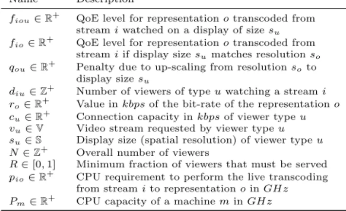
Name Description
fiou∈R+ QoE level for representationotranscoded from streamiwatched on a display of sizesu
fio∈R+ QoE level for representationotranscoded from streamiif display sizesumatches resolutionso
qou∈R+ Penalty due to up-scaling from resolutionsoto display sizesu
diu∈Z+ Number of viewers of typeuwatching a streami ro∈R+ Value inkbpsof the bit-rate of the representationo cu∈R+ Connection capacity inkbpsof viewer typeu vu∈V Video stream requested by viewer typeu su∈S Display size (spatial resolution) of viewer typeu N∈Z+ Overall number of viewers
R∈[0,1] Minimum fraction of viewers that must be served
pio∈R+ CPU requirement to perform the live transcoding from streamito representationoinGHz Pm∈R+ CPU capacity of a machineminGHz
Table 4: ILP notation.
representation o ∈ O corresponds to a triple (vo, ro, so),
that is, to a video representation of type of contentvo ∈ V
encoded at the resolutionso∈ S and at the bit-ratero∈ R.
Let M be the set of physical machines where the transcoding tasks should be performed. Each machine m ∈ M can accommodate transcoding jobs up to a maximum CPU load ofPm GHz.
To reduce the size of the problem, and make it more tractable, we introduce the notion ofviewer type. LetU be the set of viewers types. All viewers in a given viewer type u ∈ U have the same display resolution (i.e., the spatial resolution at which the video is displayed on the device) su ∈ S, request the same video type vu ∈ V, and use an
Internet connection with the same bandwidth of cu kbps.
However, viewers of the same type u watch different channels. We denote bydiu the number of viewers of type
uwatching a given channeli. Note that a viewer of a given typeucan play segments encoded at resolutions lower than its display sizesuby performing spatial up-sampling before
rendering.
A viewer from viewer type u watching a video representation otranscoded from a stream iexperiences a QoE level of fiou, which is an increasing function of the
bit-rate ro. Based on the dataset presented in Section 3.2,
we know that the QoE function depends on the video content type vo, the resolution so and the original raw
video streami. As previously said, the QoE levelfiou also
depends on whether the video should be up-scaled or not, since up-scaling introduces a penalty on the final QoE value. We incorporate this up-scaling penalty into the QoE computation by the following definition offiou:
fiou=
fio, ifso=su
fio−qou, ifso< su i∈ I, o∈ O, u∈ U (1)
where fio is the QoE level when the display resolution and
the target video resolution match, andqou is the penalty of
the up-scaling process from resolution so to the viewer
display size su. Table 4 summarizes the notation used
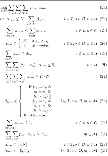
Integer Linear Programming formulation max {ααα,βββ} X i∈I X o∈O X u∈U
fiou·αiou (2a)
s.t. αiou≤N· X m∈M βiom, i∈ I, o∈ O, u∈ U (2b) X m∈M βiom≤ X u∈U αiou, i∈ I, o∈ O (2c) αiou≤ N, ifsu≥so 0, otherwise i∈ I, o∈ O, u∈ U (2d) X o∈O αiou≤diu, i∈ I, u∈ U (2e) X i∈I X o∈O ro−cu ·αiou≤0, u∈ U (2f) X i∈I X o∈O X u∈U αiou≥R·N, (2g) βiom≤ 1,if (vi=vo & si=so & bi> bo)k (vi=vo & si> so & bi≥bo) 0,otherwise i∈ I, o∈ O, m∈ M (2h) X m∈M βiom≤1, i∈ I, o∈ O (2i) X i∈I X o∈O pio·βiom≤Pm, m∈ M (2j) αiou∈[0, N], i∈ I, o∈ O, u∈ U (2k) βiom∈ {0,1}, i∈ I, o∈ O, m∈ M (2l)
5.2
ILP Model
We now describe the ILP. The decision variables in the model are:
αiou ∈ Z≥0 : Number of viewers of type u watching a representationotranscoded from a streami.
βiom=
1, if machinemtranscodes streamiinto representationo
0, otherwise.
With these definitions, the optimization problem can be formulated as shown in (2).
The objective function (2a) maximizes the average viewer QoE. The constraints (2b) and (2c) set up a consistent relation between the decision variablesαandβ. The constraint (2d) establishes that a viewer of typeucan play only the transcoded representations o with spatial resolutions equal or smaller than the viewer display sizesu,
that is, those susceptible to experience an up-sampling operations at the rendering. The constraints (2e) ensures that the sum of all the viewers of type u watching any representationotranscoded from a given streamidoes not exceed the number of viewers of typeuoriginally watching the stream i. The constraint (2f) limits the viewer link capacity. The constraint (2g) force us to serve at least a certain fraction R of viewers. The constraint (2h) forces that only transcoding operations defined over the same video content type are allowed and it forbids senseless transcoding operations, like transcoding to higher bit-rates
or higher resolutions or transcoding to the same rate-resolution pair. The constraint (2i) guarantees that a given transcoding task (i, o) is performed in one unique machine m. Finally, (2j) sets the CPU capacity of each machinem.
5.3
Settings for Performance Evaluation
To find the exact solution of the optimal problem, we use the generic solver IBM ILOG CPLEX [10] on a set of instances. Unfortunately, this approach does not allow solving instances as large as the ones that live service providers face today. Thus, we have built problem instances based on the datasets introduced in Section 3 but of a smaller size.Incoming Videos from Broadcasters. We restrict the size of the set of sources by picking only the 50 most popular channels from the Twitch dataset (see Section 3.1). More precisely, we take 66 snapshots from the dataset, corresponding to those ones extracted every 4 hours along 11 days since April, 10th 2014 at 00:00. For each snapshot, we use the channel information (bit-rate and resolution), which we modify slightly to match the spatial resolutions and bit-rates from Table 6. Each channel is randomly assigned to one of the four video types given in Table 2.
QoE for Target Videos. We use the dataset presented in Section 3.2 to obtain the QoE (estimated as a PSNR score) fioof a target videooobtained from transcoding a sourcei.
The up-scaling penaltiesqouare fixed using PSNR measures
from the situation shown on bottom of the Figure 7 (target resolution lower than display one).
CPU for the Transcoding Tasks. Still to reduce the size of the instances, and thus the complexity of the problem, we fit an exponential function to the set of CPU measurements:
p=a·rb (3)
where p is the number of GHz required to transcode a source into a target,aandbare the parameters used in the curve fitting and the parameterris the bit-rate in Mbps of the target video. The values of the parameters a and b depend on (i) the source video (content type, bit-rate and resolution), and (ii) the resolution of the target video. The fitting curves are identified by continuous lines in Figure 5. Table 5 gives the parameters a and b used in the curves shown in Figure 5. Target Resol a b 224p 0.673091 0.024642 360p 0.827912 0.033306 720p 1.341512 0.060222 1080p 1.547002 0.080571
Table 5: Parameters of the fitting model of the transcoding CPU curves. Source stream: 1080p, 2,750 kbps, movie
Viewers. The viewers set U is based on the dataset [4] presented in Section 3.3. However, the number of viewers is too large and we implement the concept of user type. To build the types, we divide the range of bandwidth into bins, whose limits are selected so that each bin contains an equal number of viewers. A viewer type corresponds to a bin, with a display spatial resolution set according to the lower bandwidth in the bin, and the downloading rate of
the viewer type is equal to the lower bandwidth in the bin. The number of viewers diu watching a raw video i is
proportionally set up according to the popularity of the channel in the Twitch dataset.
5.4
Numerical Results
We now show the results of our analysis. We use the previous settings and we also fix the CPU capacityPm of
all the machines to 2.8 GHz, the speed clock of the physical processors used by the amazon cloud computing C3 instances9. Our motivation is to determine how far from the optimal are current industry-standard strategies. In Figure 9, we represent the average QoE, expressed as the PSNR in dB, as a function of the number of machines. The line represents the results obtained from solving the optimization problem with CPLEX. We show with grey pins the results for both industry-standard strategies. The results are the average over all the snapshots we took from the Twitch datasets.
We first emphasize that the amount of hardware resources in the data-center has a significant impact on the QoE for the viewers. The difference of PSNR reaches 4 dB between 10 and 100 machines. This remark matters because it highlights the need of being able to reserve the right amount of resources in the data-center. However, the ability to forecast the load and to reserve the resources is not trivial for elastic live streaming services such as Twitch.
Our second main observation is that, on our datasets, the Full-Cover strategy is more efficient than the Zencoder one in terms of trade-off QoE-CPU. The Full-Cover strategy is close to the optimal, and thus represents an efficient implementation with respect to its simplicity. Note however that Full-Cover needs 48 machines, while there exists a solution with the same QoE but with only 35 machines. Therefore, a significant reduction of resources to reserve can be obtained. The Zencoder strategy is outperformed by the Full-cover one, as it consumes nearly twice the CPU cycles for a tiny increase of the QoE. For a similar amount of CPU, the QoE gap between the Zencoder strategy and the optimal is more than 0.9 dB, which is significant. 20 40 60 80 100 29 30 31 32 33 Full-Cover Zencoder number of machines A vg . PS N R (in d B )
Figure 9: Optimal average QoE for the viewers vs. the number of machines that are used in the data-centers. The 50 most popular channels from several snapshots of the Twitch datasets are transcoded.
9
http://aws.amazon.com/ec2/instance-types/
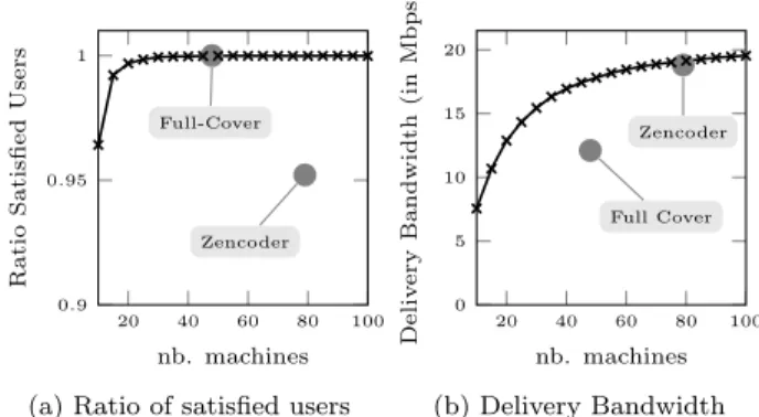
To complete this study, we provide another view of the choices to be taken in Figure 10. Here, we show the ratio of served users and the amount of delivery bandwidth required to serve the users. In our ILP, we optimize the average QoE so the solutions found by CPLEX are not optimal on other aspects. In Figure 10b, we see that the delivery bandwidth of the optimal solution is significantly higher than the Full-Cover, which may annihilate the gains obtained by using fewer machines. Please note that both parameters of Figure 10 can also be the objective of the ILP. In the same vein, the ILP can also be re-written so that the parameter to be optimized is the amount of CPU needed, subject to a given QoE value.
20 40 60 80 100 0.9 0.95 1 Full-Cover Zencoder nb. machines Ra ti o S a ti sfi e d Us e rs
(a) Ratio of satisfied users
20 40 60 80 100 0 5 10 15 20 Full Cover Zencoder nb. machines De li v e ry Ba n d wi d th (i n M b p s) (b) Delivery Bandwidth Figure 10: Other views on the optimal solution of Figure 9
6.
A HEURISTIC ALGORITHM
We now present and evaluate an algorithm for massive live streaming preparation. Our goal is to design a fast, light, adaptive algorithm, which can be implemented in production environments. This algorithm should in particular be able toabsorb the variations of the streaming service demand while using a fixed data-center infrastructure.
6.1
Algorithm Description
The purpose of the algorithm is to update the set of transcoded representations with respect to the characteristics and the popularity of the incoming raw videos. The algorithm is executed on a regular basis (for example every five minutes to stick to the Twitch API) by the live streaming service provider in charge of the data-center. You can find in Appendix B the pseudo-code of the algorithms and some additional details.
Algorithm in a Nutshell. We process each channel iteratively in a decreasing order of their popularity. For a given channel, the algorithm has two phases: First, we decide a CPU budget for this channel. Second, we determine a set of representations with respect to the CPU budget computed during the first phase.
Set a CPU Budget Per Channel. We base our algorithm on the observations of the optimal solutions found by CPLEX. Four main observations are illustrated in Figure 14 in the Appendix: (i) the ratio of the overall CPU budget of a given channel is roughly proportional to the ratio of viewers watching this channel; (ii) the CPU budget per channel is less than 10 GHz; (iii) some video types
(e.g., sport) require more CPU budget than others (e.g., cartoon); and (iv) the higher is the resolution of the source, the bigger the CPU budget.
We derive from these four observations the algorithm shown in Algorithm 1. We start with the most popular channel. We first set anominal CPU budget according to the ratio of viewers and the maximal allowable budget. Then we adjust this nominal budget based on avideo type weight and aresolution weight (interested readers can find in the Appendix details about the values we chose for these weights, based on observations from the optimal solutions). We obtain a CPU budget for this channel.
Decide the Representations for a Given CPU Budget. The pseudo-code is detailed in Algorithm 2. This algorithm builds the set of representations by iteratively adding the best representation. At each step, the needed CPU budget to transcode the chosen representation should not exhaust the remaining channel budget. To decide among the possible representations, we need to estimate the QoE gain that every possible representation can provide if it is chosen. To do so, we estimate the assignment between the representations and the viewers in Algorithm 3. In short, this algorithm requires a basic knowledge on the distribution of downloading rates in the population of viewers, which is usually the case for service providers. (In this work, we study the worst case scenario where service providers do not have this information and they assume a uniform distribution in the range between 100 kbps and 3,000 kbps). The idea is then to assign subsets of the population to representations and to evaluate the overall QoE. Details are given in the Appendix.
6.2
Simulation Settings
Our simulator is based on the datasets presented in Section 3 and the extra settings given in Section 5.3. However, in contrast to the ILP, our heuristic is expected to scale. Therefore we evaluate the heuristic and the aforementioned industry-standard strategies on the complete dataset containing all online broadcasters at each snapshot. Regarding the viewers, we consider now each viewer, to which we randomly assign a bandwidth value as presented in Section 3.3 and a display resolution accordingly. We use the actual number of viewers watching channels according to the Twitch dataset.
Please note also that we focus here on the decision about the representations (number of representations and transcoding parameters), and we neglect the assignment of transcoding jobs to machines. This does not impact the evaluation since all tested strategies (our heuristic and both industry-standard strategies) can be evaluated without regard to this assignment. We let for future works the integration of the VM assignment policy into middleware such as OpenStack.10
6.3
Performance Evaluations
In the following, we present the same set of results from two different perspectives; first, we show how the performances evolve throughout the eleven days we consider. Then, we present the results in order to highlight the main features of the algorithms.
10
http://www.openstack.org/
In Figure 11 we show the three main metrics during our 11-days dataset. The combination of the three figures reveals the main characteristics of the strategies. The main point we would like to highlight is that our heuristic keeps a relatively constant, low CPU consumption without regard to the traffic load in input. Our heuristic also succeeds in maintaining a high QoE. To achieve this excellent trade-off, our heuristic adjusts with the ratio of served viewers. Yet, this ratio maintains a high value since it is always greater than 95%. Our heuristic thus demonstrates the benefits from having different representation sets for the different channels according to their popularity. The industry-standard strategies are less capable of absorbing the changing demand. In particular, the CPU needs of the Zencoder strategy ranges from 1,000 GHz to 18,000 GHz while the average QoE is always lower than for our heuristic.
To highlight the relationship between CPU needs and QoE for the population, we represent in Figure 12 a cloud of points for each snapshot. The Full-Cover has most points in the southwest area of the Figure, which corresponds to a low CPU utilization but also a low QoE. We also note that the distance between two points can be high, which emphasizes an inability to absorb load variations. This inability is even stronger for the Zencoder strategy, for which the points are far from each other, covering all areas of the Figure. On the contrary, our heuristic absorbs well elastic services, with points that are concentrated in the northwest part of the Figure, which means low CPU and high QoE.
7.
CONCLUSIONS
This paper studies the management of new live adaptive streaming services in the cloud from the point of view of streaming providers using cloud computing platforms. All the simulations conducted in the paper make use of real data from three datasets covering all the actors in the system. The study is focused on the interactions between the optimal video encoding parameters, the available CPU resources and the QoE perceived by the end-viewers. We use an ILP to model this system and we compare its optimal solution to current industry-standard solutions, highlighting the gap between the two. Due to the ILP computational limitations, we propose a practical algorithm to solve problems of real size, thanks to key insights gathered from the optimal solution. This algorithm finds representations beating the industry-standard approaches in terms of the trade-off between viewers QoE and CPU resources needed. Furthermore, it uses an almost-constant amount of computing resources even in the presence of a time varying demand.
8.
REFERENCES
[1] Twitch.tv: 2013 retrospective, Jan. 2014. http://twitch.tv/year/2013.
[2] M. Adler, R. K. Sitaraman, and H. Venkataramani. Algorithms for optimizing the bandwidth cost of content delivery.Computer Networks,
55(18):4007–4020, 2011.
[3] L. A. Barroso, J. Clidaras, and U. H¨olzle.The Datacenter as a Computer: An Introduction to the Design of Warehouse-Scale Machines. Morgan & Claypool, 2013. Second Edition.
Full-Cover Zencoder Heuristic 1 2 3 4 5 6 7 8 9 10 11 31.5 32 32.5 33 Days A vg . V iew er PSN R ( DB )
(a) Average Viewer PSNR
1 2 3 4 5 6 7 8 9 10 11 0.9 0.95 1 Days R at io Sa t is fi ed V iew er s
(b) Ratio of satisfied viewers
1 2 3 4 5 6 7 8 9 10 11 0 5 000 10 000 15 000 20 000 Days T o t al CPU ( GH z)
(c) Total CPU needs
Figure 11: Different metric results over time for the distinct solutions: Full-Cover strategy, Zencoder encoding recommendations and our Heuristic.
Satisfied Viewers Ratio: 95-96% 97-98% 99-100%
0 5 000 10 000 15 000 20 000 31 31.5 32 32.5 33 Total CPU (GHz) A vg . PSN R (dB ) (a) Full-Cover 0 5 000 10 000 15 000 20 000 31 31.5 32 32.5 33 Total CPU (GHz) (b) Heuristic 0 5 000 10 000 15 000 20 000 31 31.5 32 32.5 33 Total CPU (GHz) (c) Zencoder
Figure 12: Total required CPU (in GHz) by the perceived QoE for strategies Full-Cover, Zencoder encoding recommendations and Heuristic. The markes shape indicates the percentage of satisfied viewers. Each point corresponds to one of the 66 snapshots.
[4] S. Basso, A. Servetti, E. Masala, and J. C. D. Martin. Measuring DASH streaming performance from the end users perspective using neubot. InACM MMSys, 2014. [5] N. Bouzakaria, C. Concolato, and J. L. Feuvre.
Overhead and performance of low latency live streaming using MPEG-DASH. InIEEE IISA, 2014. [6] R. Cheng, W. Wu, Y. Lou, and Y. Chen. A
cloud-based transcoding framework for real-time mobile video conferencing system. InIEEE MobileCloud, 2014.
[7] J. Guo and L. Bhuyan. Load balancing in a
cluster-based web server for multimedia applications. IEEE Transactions on Parallel and Distributed Systems, 17(11):1321–1334, Nov. 2006.
[8] Z. He, Y. Liang, L. Chen, I. Ahmad, and D. Wu. Power-rate-distortion analysis for wireless video communication under energy constraints.IEEE Transactions on Circuits and Systems for Video Technology, 15(5):645–658, 2005.
[9] Z. Huang, C. Mei, L. Li, and T. Woo. CloudStream: Delivering high-quality streaming videos through a cloud-based SVC proxy. InIEEE INFOCOM, 2011. [10] IBM. Ilog cplex optimization studio.
http://is.gd/3GGOFp.
[11] F. Jokhio, A. Ashraf, S. Lafond, I. Porres, and
J. Lilius. Prediction-based dynamic resource allocation for video transcoding in cloud computing. In
Euromicro PDP, 2013.
[12] F. Lao, X. Zhang, and Z. Guo. Parallelizing video transcoding using map-reduce-based cloud computing. InIEEE ISCAS, 2012.
[13] S. Lin, X. Zhang, Q. Yu, H. Qi, and S. Ma.
Parallelizing video transcoding with load balancing on cloud computing. InIEEE ISCAS, 2013.
[14] J. Liu, G. Simon, C. Rosenberg, and G. Texier. Optimal delivery of rate-adaptive streams in
underprovisioned networks.IEEE Journal on Selected Areas in Communications, 2014.
[15] K. Pires and G. Simon. DASH in Twitch: Adaptive Bitrate Streaming in Live Game Streaming Platforms. InACM VideoNext Conext Workshop, 2014.
[16] C. Rea˜no Gonzalez. CU2rCU: A CUDA-to-rCUDA Converter. Master’s thesis, Universitat Politecnica de Valencia, 2013.
[17] H. Reddy. Adapt Or Die: Why Pay-TV Operators Must Evolve Their Video Architectures, July 2014. Videonet white paper.
[18] J. Reichel, H. Schwarz, and M. Wien. Joint scalable video model 11 (jsvm 11).Joint Video Team, Doc. JVT-X202, 2007.
[19] R. Shea and J. Liu. On GPU pass-through performance for cloud gaming: Experiments and analysis. InACM Netgames, 2013.
[20] H. Sohn, H. Yoo, W. De Neve, C. S. Kim, and Y.-M. Ro. Full-reference video quality metric for fully scalable and mobile svc content.IEEE Transactions on Broadcasting, 56(3):269–280, Sept 2010.
[21] L. Su, Y. Lu, F. Wu, S. Li, and W. Gao.
Complexity-constrained h.264 video encoding.IEEE Transactions on Circuits and Systems for Video Technology, 19(4):477–490, Apr. 2009.
[22] L. Toni, R. Aparicio-Pardo, G. Simon, A. Blanc, and P. Frossard. Optimal set of video representations in adaptive streaming. InACM MMSys, 2014.
[23] Z. Wang, L. Sun, C. Wu, W. Zhu, and S. Yang. Joint online transcoding and geo-distributed delivery for dynamic adaptive streaming. InIEEE INFOCOM, 2014.
[24] XIPH. :xiph.org video test media. [25] M. Yang, J. Cai, Y. Wen, and C. H. Foh.
Complexity-rate-distortion evaluation of video encoding for cloud media computing. InIEEE ICON, 2011.
APPENDIX
A.
TRANSCODING CPU USAGE
In this Appendix we give more details about the experiments that we have used to estimate the CPU usage of different transcoding operations.
A.1
Input and Output Rates
As discussed in Section 3.2, we consider only the rates covering 90% of the sources that we observe in the Twitch dataset, as detailed in Table 6. For low resolutions (224p and 360p), the set of bit-rates ranges from 100 kbps up to 3000 kbps with steps of 100 kbps, while for high resolutions (720p and 1080p), the set of bit-rates ranges from 1000 kbps up to 3000 kbps with steps of 250 kbps. Thus, each video sequence from Table 2 can be encoded into 78 different combinations of rates and resolutions. To obtain these 78 sources, we took the original full-quality decoded videos from Table 2 and we encoded them into each of the 78 videos that we consider as possible raw videos.
Resol. WidthxHeight Min–Max Rates Rate Steps
224p 400 x 224 100–3000 kbps 100 kbps 360p 640 x 360 100–3000 kbps 100 kbps 720p 1280 x 720 1000–3000 kbps 250 kbps 1080p 1920 x 1080 1000–3000 kbps 250 kbps
Table 6: Resolutions and ranges of rates for the raw videos.
A.2
Transcoding
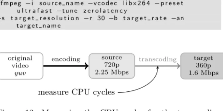
The transcoding operation that we have performed is summarized in Figure 13. This operation has been done 12,168 times in total. This corresponds to 4 (the number of video types) multiplied by 78 (the number of possible sources) multiplied by 39 (the average number of possible target videos). Recall that, for each input video, we produced only videos with resolutions and bit-rates lower than or equal to those of the input. That is, only a subset
of the 78 possible representations are created from a given raw video.
We have usedffmpegfor the transcoding with the same parameters as in [5], which is a study conducted by the leading developers of the popular GPAC video encoder. The command is f f m p e g −i s o u r c e n a m e −v c o d e c l i b x 2 6 4 −p r e s e t u l t r a f a s t −t u n e z e r o l a t e n c y −s t a r g e t r e s o l u t i o n −r 30 −b t a r g e t r a t e −an t a r g e t n a m e original video yuv source 720p 2.25 Mbps target 360p 1.6 Mbps encoding transcoding
measure CPU cycles
Figure 13: Measuring the CPU cycles for the transcoding of any source to any target video. Here an example with a source at 720p and 2.25 Mbps and a target video at 360p and 1.6 Mbps.
Measuring CPU cycles. As discussed above and in Section 3.2, we have run many transcoding operations using an Intel Xeon CPU E5640 at 2.67GHz with 24 GB of RAM using Linux 3.2 with Ubuntu 12.04. To measure the number of used CPU cycles, we use the perf tool11, a profiler for Linux 2.6+ based systems, with the next command:
p e r f s t a t −x −e CYCLES
This command provides access to the counter collecting the number of CPU cycles at the Performance Monitoring Unit (PMU) of the processor. Then, this number is divided by the duration in s of the video sequences to obtain the frequency of CPU (in GHz) required to perform the transcoding during a running time equal to the play time of the video, that is, the frequency of CPU required to do a live transcoding.
B.
HEURISTIC
B.1
Settings
CPU Budget Per Channel. The values we used for both video type weight and resolution weight are given in Tables 7. These values correspond the average of the curves plotted in Figure 14, which we obtain from the optimal solutions computed by CPLEX on the 50 most popular channels and 100 machines. Thex-axis is the rank of the channels according to their popularity. On the top we show the average distribution of CPU budget per channel. On the bottom, we show the average difference between the average CPU budget when a channel from a given type (respectively resolution) is at a given rank and the average CPU budget for channels at this rank. This difference allows us to compute the adjustment of CPU budget according to the video type and the resolution. 11
Video Type Weight Cartoon -0.176 Documentary 0.072 Sport 0.190 Video -0.076 Resolution Weight 224p -0.917 360p -0.657 720p -0.108 1080p 0.432
Table 7: Video type and resolution weights
0.02 0.04 CPU % −0.4 −0.2 0 0.2 0.4 CPU Di ff .
Cartoon Documentary Sport Video
0 10 20 30 40 50
−1
−0.5 0 0.5
Channel Rank Position by its Popularity
CPU
Di
ff
.
224p 360p 720p 1080p
Figure 14: CPU information for a given channel popularity rank. Data comes from the average optimal solution with 100 machines. From the average total CPU % according to the rank (top figure), we derive the difference between distinct video types (middle figure) and between distinct channel input resolutions (bottom figure).
Estimation Viewers QoE. To estimate the QoE gain when choosing one representation, we need to consider all the assignments representations-viewers. In Algorithm 3, we evaluate the representations in the set in descending order of their bit-rates. At each iteration, we identify the fraction of viewers whose bandwidth is between the rate of the considered representation and the closest representation with superior bit-rate. Then, we also have to take into account the display sizes of the viewers (it also depends on the knowledge of the service provider; we again considered it a minimal knowledge of the population). Therefore, this fraction of viewers is again split into one or more sub-fractions corresponding to their display resolutions. A different value of PSNR is then computed for each sub-fraction. This value is multiplied by the ratio of viewers belonging to the sub-fraction. When all the representations have been assessed, the sum of the PSNR contributions of all the sub-fractions of viewers is returned as the estimated QoE of the set.
B.2
Algorithms in Pseudo-code
This section includes the pseudo-codes of the heuristic described in Section 6.
Algorithm 1:Main routine
Data: channelsSet: Channels metadata (e.g. number of viewers, id) sorted by decreasing channel popularity.
Data: totalCPU: total CPU Budget in GHz.
1 representations←emptySet() 2 foreachchannel∈channelsSetdo
3 cpu←channel.viewersRatio∗totalCP U 4 cpu←min(cpu, M AX CP U)
5 w video←getV ideoT ypeW eight(channel.video) 6 w resol←getResolutionW eight(channel.resolution) 7 cpu←max(cpu∗(1 +w video+w resol),0) 8 representations.append(findReps(channel, cpu)) 9 returnrepresentations
Algorithm 2: findRepsFind the channels representations set meeting a budget
Data: channel: Channel metadata (e.g. number of viewers, id).
Data: CPU: calculated channel CPU Budget in GHz.
1 representations←emptySet() 2 f reeCP U←CP U
3 repeat
4 newRep←f alse
5 foreach
resolution≤channel.resolution∈resolutionsSetdo 6 foreachbitRate∈bitRatesSet[resolution]do 7 thisRep←(resolution, bitRate)
8 ifbitRate≤channel.bitRateand
thisRep /∈representationsthen
9 thisRep.cpu←getCP U(thisRep, channel)
10 ifthisRep.cpu≤f reeCP Uthen 11 reps←representations+thisRep
12 thisRep.qoe←getQoE(reps, channel)
13 ifnotnewRepor
newRep.qoe < thisRep.qoethen
14 newRep←thisRep
15 ifnewRepthen
16 representations.append(newRep) 17 f reeCP U−=newRep.cpu 18 untilnotnewRep
19 returnrepresentations
Algorithm 3: getQoEObtain an estimation of PSNR for a given representation set of one channel
Data: channel: Channel metadata (e.g. number of viewers, id).
Data: repSet: Set of representations for a given channel.
1 totalP SN R←0 2 foreachrep∈repSetdo
3 ranges←getResolutionsRanges(rep)
4 foreachviewersRange∈rangesdo
5 v ratio←getV iewersRatio(viewersRange) 6 v resol←getV iewersResolution(viewersRange) 7 partialP SN R←calcP SN R(rep, channel, v resol) 8 totalP SN R+ =v ratio∗partialP SN R