C-Cell: An Efficient and Scalable Network
Structure for Data Centers
Hui Cai
Logistical Engineering University of P.L.A, Chongqing, China Email: caihui_cool@126.com
ShengLin Li
Logistical Engineering University of P.L.A, Chongqing, China Email: 492739390@qq.com
Wei Wei
Logistical Engineering University of P.L.A, Chongqing, China Email: vivianww@yeah.net
Abstract—Data centers play a crucial role in current
Internet architecture supporting content-centric networking. How to efficiently interconnect an exponentially increasing number of servers is a fundamental challenge in data centers networking. This paper presents C-Cell, a new network architecture which is designed on the basis of recursive structure. A high-level C-Cell is constructed by low-level C-Cell. And this structure not only has a low-ratio in switch/server, but also provides multiple parallel short paths between any pair of servers. On the premise of low proportion of switches and servers, C-Cell can efficiently achieve routing mechanisms in shorter mean path lengths with less network cost.
Index Terms— Data center, network, routing, protocol
I. INTRODUCTION
In recent years, data center networking (DCN) has been attracting much attention of researchers, which designs both the network structure and associated protocols that interconnect thousands of servers at a data center. But the development of DCN not only leads to great challenges to the high and balanced network capacity, and robustness to link/server faults, but also results in high hardware infrastructure cost and power cost. Therefore, fault-tolerance, scalability, and power consumption of the distributed storage for a data center become key parts in order to ensure the data availability and reliability.
In this paper, the authors focus on a simple technical problem. Can we build a fault-tolerance, scalability and low-cost networking infrastructure for data centers, using only commodity server with 3 ports and commodity switch? There are many potential benefits to solve this problem. Firstly, we do not use the high-end and expensive switch which is widely used today. And commodity server can also be available. Secondly, the wiring becomes easier if only 3 ports server is used for interconnection. There is no need to add additional
hardware or wire on a server. Thirdly, more academic research into data centers can be spawned. New problems in data center networking can be found and assessed through some easy-build tests in institution.
But recent proposals and current practice cannot solve those problems. The tree-based structure needs expensive and high-end switch as the core switch at the top level of the tree. And the core switch failure may tear down thousands of servers. The Fat-Tree solution needs more switches, and the number of ports at a switch limits the scale of the Fat-Tree[1]. DCell[2] and BCube[3] also require more ports in a server (typically four), to establish a large server population. The fundamental problem is that, we need to design a new data center networking structure that works for servers with node degree of only 3 in order to scale.
We propose C-Cell, an Efficient and Scalable network structure for a data center. C-Cell defines a recursive structure to interconnect servers. A high-level C-Cell is constructed by low-level C-Cell. And this structure not only has a low-ratio in switch/server, but also provides multiple parallel short paths between any pair of servers. Therefore, C-Cell has fault tolerance and load balance.
The rest of the paper is organized as follow. Section 2 discusses the background. Section 3 describes the C-Cell structure and its properties. Section 4 presents the C-Cell routing and section 5 discusses the solution to incremental expansion. Section 6 uses both simulations and experiments to evaluate the C-Cell. Section 7 concludes the paper.
II. BACKGROUND
In this section, we firstly explain the traditional hierarchy data center, and then discuss the insufficiency. Secondly, we introduce the current data center and analyze their features.
Traditional data center uses the hierarchy structure. As shown in Fig 1, a layer of servers at the bottom is connected to a Top of Rack (ToR) switch. ToR is
connected to two L2 switches for redundancy. L2 switches further connect to L3 routers. At the top of this structure, core routers are very important because they manage the traffic into and out of the data center and carry all traffic between L3 routers. But there are some fundamental limitations to this conventional design[4-6].
CR CR AR AR AR AR AS AS S S S S TOR SERVERS TOR SERVERS TOR SERVERS TOR SERVERS INTERNET Data Center Layer 3 Layer 2 ... ... ... ... Key CR=L3 Core Router AR=L3 Access Router AS=L2 Aggr Switch S=L2 Switch TOR=Top-of-Rack Switch
Figure 1. A network architecture for tradition data centers Limited scale: Servers which are connected in the same access router constitute a single layer-2. Because of the conventional design, the scale of a single layer-2 only has 4 thousand servers. It means that traditional data center cannot afford ascale of millions of servers.
Limited server-to-server: If we go up the hierarchy, the traffic moving up the different layer-2 needs to go through layer-3. And the link between layer-2 to layer-3 is oversubscription. So, the bandwidth in layer-2 is limited by the oversubscription ratio. For example, the uplinks from layer-2 are 1:20 oversubscribed, and paths through layer-3 can be 1:240 oversubscribed. This large oversubscription factor fragments the server pool by preventing idle servers from being assigned to overloaded services, and it severely limits the entire data center’s performance.
Fragmentation of resources: As the cost and performance of communication depends on distance in the hierarchy, the conventional design encourages service planners to cluster servers nearby the hierarchy. Moreover, spreading a service outside a single layer-2 domain frequently requires the onerous task of reconfiguring IP addresses and VLAN trunks, since the IP addresses used by servers are topologically determined by the access routers above them. Collectively, this contributes to the squandering of computing resources across the data center. The consequences are egregious. Even if there is plentiful spare capacity throughout the data center, it is often effectively reserved by a single service (and not shared), so that this service can scale out to nearby servers to respond rapidly to demand spikes or to failures. In fact, the growing resource need one service to have forced data center operations so as to evict other services in the same layer-2 domain, incurring significant cost and disruption.
Poor reliability and utilization: Above the ToR, the basic resilience model is 1:1. For example, if an aggregation switch or access router fails, there must be
sufficient remaining idle capacity on the counterpart device to carry the load. This forces each device and link to run up to at most 50% of its maximum utilization. Inside a layer-2 domain, the use of the Spanning Tree Protocol means that even when multiple paths between switches exist, only a single one is used. In the layer-3 portion, Equal Cost Multipath (ECMP) is typically used: when multiple paths of the same length are available to a destination, each router uses a hash function to spread flows evenly across the next available hops. However, the conventional topology offers at most two paths.
High cost of hardware: core-switches and core-routers which are used in traditional data center network are expensive. And the load balancer in layer-2 must be used in pairs.
There are some requirements and features in the new data center[7-8]:
• The data center infrastructure must be scalable to a large number of servers and allow for incremental expansion.
• The data center must be fault tolerant against various types of server failures, link outages, or server-rack failures.
• The data center must be able to provide high network capacity to better support bandwidth-hungry services.
• The data center must support virtualization which is the biggest difference between traditional data center and new data center.
Currently, data centers use commodity-class computers and switches instead of specially designed high-end servers and interconnect for better price-performance ratio. There are some representative data centers liking Fat-tree[1,12], DCell[2], BCube[3] and VL2[11].
The Fat-tree is a layered network topology with equal link capacity at every tier and is commonly implemented by building a tree with multiple roots. The structure of Fat-tree has k pods, and each pod has k/2 switches which have k ports. The k/2 ports connect k/2 servers, and another k/2 ports connect core-switches. The core layer has k core-switches which have k ports. The Fat-tree has several parallel paths between nodes, and removes the constraints about upper link throughput. But the Scalability of Fat-tree is limited by the number of port of core-switch, and Fat-tree is very sensitive to the fault of low-layer switch.
DCell uses a recursively-defined structure to interconnect servers. Each server connects different levels of DCells via multiple links. We build high-level DCells recursively from many low-level ones, in a way that the low-level DCells form a fully-connected graph. Usually, the number of servers in DCell0 is 3 to 8. When a DCell0
has 6 servers, the number of servers in a DCell3 is
3.26-million. But there are some defects in DCell. The fully-connected graph used in DCell is too complex to manage and maintain. And the flow of DCell at different level is uneven.
BCube is the modular version of DCell. A BCube0 is
simply n servers connecting to an n-port switch. A BCube1 is constructed from n BCube0s and n n-port
switches. Generically, a BCubek (k≥1) is constructed
from n BCubek-1s and nk n-port switches. Each server in a
BCubek has k+1 ports, which are numbered from level-0
to level-k. BCube can significantly accelerate one-to-x traffic patterns and provides high network capacity for all-to-all traffic. The BCube Source Routing (BSR) further enables graceful performance degradation. But the weakness of BCube is a relatively poor scalability. When k=3and n=8 (k is the degree of BCube, n is the number of servers in a BCube0), BCube3 only has 4096 servers.
VL2 is a scalable and flexible data center network. VL2 uses flat addressing to allow service instances to be placed anywhere in the network, Valiant Load Balancing to spread traffic uniformly across network paths, and end system-based address resolution to scale to large server pools without introducing complexity to the network control plane.
III. THE C-CELL NETWORK STRUCTURE
In this section, we firstly present the C-Cell structure and then analyze its efficiency and some properties. Sections 3-5 describe these components in detail.
A. Cell Physical Structure and the Way to Build C-Cell
There are two types of devices in C-Cell: Servers with multiple ports, and switches that connect a constant number of servers. We know that DCell and BCube are a recursively defined structure. In C-Cell, we also use a recursive way to define its structure. The C-Celln is
constructed by a C-Celln-1 and several C-Cell0s. This
structure has some advantages. Firstly, the modularized and recursive structure is good for connection. Secondly, it is easy to expand C-Celln+1 when C-Celln is incomplete.
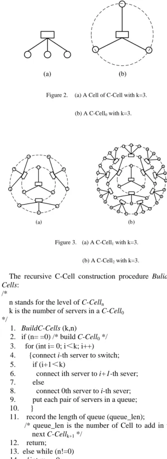
A C-Cell0 which is the building block to construct
larger C-Cell is simply k servers connecting to a m-port (m>k) switch. The following example in Fig 2(a) illustrates a C-Cell0 (k=3). 3 servers are connected to a
switch. We then equally adjust each server to the circle0
which has the switch as the center, and an arc of the circle0 between every two servers bridges the connection
of two servers, as illustrated in Fig 2(b). In order to distinguish the difference between Fig 2(a) and Fig 2(b), the structure of Fig 1(b) we called C-Cell0 (k=3), and the
structure of Fig 1(a) we called Cell. On the basis, a C-Cell1 is structured from a C-Cell0 and k Cells. The
method is to break k arcs which connect two adjacent servers and adding a Cell. A C-Cell1 (k=3) is illustrated in
Fig 3(a). More generically, a C-Celln (n≥ 1) is
constructed from a C-Celln-1 and kn+1 Cell. In our design,
each server in a C-Celln has 3 ports and the number of
max-port in each switch is k+2. Fig 3(b) illustrated a C-Cell2 (k=3).
The construction of a C-Celln is as follows. Firstly, we
break kn-1 arcs which connect adjacent two servers on the circlen-1. Secondly, we add a Cell in each broken arc. This
means that the two adjacent servers of C-Celln-1 on the
circlen-1 are connected by a Cell. Thirdly, we equally
adjust each newly-joined server to the circlen and connect
the newly-joined servers which are adjacent on the circlen.
Figure 2. (a) A Cell of C-Cell with k=3. (b) A C-Cell0 with k=3.
Figure 3. (a) A C-Cell1 with k=3.
(b) A C-Cell2 with k=3.
The recursive C-Cell construction procedure BulidC-Cells:
/*
n stands for the level of C-Celln
k is the number of servers in a C-Cell0
*/
1. BuildC-Cells (k,n)
2. if (n= =0) /* build C-Cell0 */
3. for (int i= 0; i<k; i++) 4. {connect i-th server to switch; 5. if (i+1<k)
6. connect ith server to i+1-th sever; 7. else
8. connect 0th server to i-th sever; 9. put each pair of servers in a queue; 10. }
11. record the length of queue (queue_len);
/* queue_len is the number of Cell to add in the next C-Cellk+1 */
12. return;
13. else while (n!=0) 14. {int m= =0;
15. while (queue_len!=0)
16. {take a pair of servers from queue, break they connection and add a Cell;
17. m=m+3; /* record the new-servers */ 18. queue_len--;
20. for (int i= 0; i<m; i++) 21. {if (i+1<m)
22. connect i-th new-server to i+1-th new-server; 23. else
24. connect 0-th new-server to i-th new-sever; 25. put each pair of new-servers in a queue; 26. }
27. record the length of queue (queue_new_len); 28. queue_len=queue_new_len;
29. n--; /* when n=0, finish */ 30. }
Figure 4. The procedure to build a C-Celln network.
B. Properties of the C-Cell
The following theorem describes and bounds the properties of C-Cell.
The number of the servers in a C-Celln is Vn and the
number of the switches in a C-Celln is Sn .
Theorem 1. n n
V
=
S
×
k
(1) 1 0 i n n iV
k
+ ==
∑
(2)for n≥0, where k is the number of servers in C-Cell0
and Cell.
Proof of Theorem 1.
A C-Celln is structured by adding Cells in a C-Celln-1.
So, the first equation can directly derive from the definitions.
Then, we use mathematical induction to prove Theorem 1. (2). When n=0, Vn=k, 1 0 i n i
k
+ =∑
=k, Vn= 1 0 i n ik
+ =∑
. When n=1, Vn=k+k×k, 1 0 i n ik
+ =∑
=k1+k2, Vn= 1 0 i n ik
+ =∑
. If n=m, 1 0 i m m iV
k
+ ==
∑
.When n=m+1, Vm+1= Vm+k×(the number of servers in
circlem ).
The number of servers in circlem=
V
m−
V
m−1= 1 1 1 0 0 i i m m i i
k
+k
+ − = =−
∑
∑
=km+1. So Vm+1= Vm+k×km+1= 1 0 i m ik
+ =∑
+km+2= 1 1 0 i m ik
+ + =∑
. The conclusion 1 0 i n n iV
k
+ ==
∑
.Theorem 1 shows that, the number of servers in a C-Cell rapidly scales as the circle degree increases. A larger network size can be lead by a small circle degree. For example, when k=6 and n=4, a C-Cell can have as many
as 9330 servers, and only 1555 switches. A ratio of switch/server is 0.167. Compare with BCube, the number of servers is 7776 when k=6 and n=4, and the number of switches is 2850. A ratio of switch/server is 0.367. Through above comparison, we can draw a conclusion that the C-Cell has more servers and lower ratio of switch/server than the BCube in the same scale. When k=3 and n=4, the ratio of switch/server in a BCube is 1.667. This condition is disadvantageous because the cost of refrigeration facilities and switches is expensive in a large data center. But when k=3(n≥0), the ratio of switch/server in a C-Cell is also 0.333.
C. Bottleneck link of the C-Cell
The bottleneck link of C-Cell can be divided into 2 aspects, node-bottleneck and path-bottleneck.
The node-bottleneck means that a node can’t afford when its data flow is too large. In a C-Cell, the lower circle a node (server/switch) is on, the more probability it becomes the node-bottleneck. So we use high-end switch instead of the node (server/switch) on low circle. This way can reduce data transmission pressure. In section 5, this question will be discuss in detail.
There is only one path to connect A subnet and B subnet. When this path is broken, the connection between A and B is lost. This path can be called path-bottleneck. But in a C-Celln, we consider that two arbitrary servers
have several parallel paths (this can be proof in theorem 5). So, a conclusion can be drawn that C-Cell does not have path-bottleneck in theory.
IV. ROUTINGIN AC-CELL
Our goal is to interconnect up to millions of servers in a C-Cell. When k=8 and n=6, 2 millions of servers are connected in a C-Cell6. The routing in a C-Cell should be
able to fully utilize the high capacity and automatically load-balance the traffic in our design. So, existing routing protocol such as OSPF is not suitable since it needs a backbone area to interconnect all the other areas. Bandwidth bottleneck and single point failure are OSPF’s biggest defect.
In this section, we firstly introduce the routing without failure in C-Cell. Secondly, we propose the routing protocol of C-Cell called C-CellRouting. Finally,an example is used to illustrate C-CellRouting.
A. Routing without Failure
We assume two servers src and des. Theorem 2.
The hamming distance of two random servers in a C-Cell0 is one.
In a C-Cell0, each server is connected to the same
switch in Fig 1(b). So theorem 2 is easy to be proved. Theorem 3.
When k=3, the shortest distance of two random servers in a C-Cell1 is at most 2. And when k>3, the shortest
distance of two random servers in a C-Cell1 is at most 3.
Proof of Theorem 3.
When k=3, there are 5 cases in a C-Cell1 ( Fig 2(a)). ①{server in C-Cell0, server in C-Cell1 }, 1.
② {server in C-Cell1, server in C-Cell0 }, 1.
③{server in C-Cell0, server in C-Cell0 }, {server in
C-Cell0, server in C-Cell1 }, 2.
④{server in C-Cell1, server in C-Cell0 }, {server in
C-Cell0, server in C-Cell1 }, 2.
⑤{server in C-Cell1, server in C-Cell0 }, {server in
C-Cell0, server in C-Cell0 }, 2.
The hamming distance of two random servers in a C-Cell0 is one (shown in theorem 2). So, when k>3, there
is another case in a C-Cell1.
{server in C-Cell1, server in C-Cell0 }, {server in
C-Cell0, server in C-Cell0 }, {server in C-Cell0, server in
C-Cell1 }, 3.
Therefore, theorem 3 is proved. Theorem 4.
In a C-Celln, the longest shortest distance of two
random servers is at most 2n+1. Proof of Theorem 4.
If src is a server on circlyi (i≤n) in a C-Celln, des is a
server on circlyj (j≤n) in a C-Celln. According to
theorem 2 and 3, we know that there are i steps when src jump to a server on circly0 (on circlyi-1, circlyi-2 ...,
circly0). In the same way, there are j steps when des jump
to a server on circly0. And the distance of two random
servers in a C-Cell0 is one (theorem 2). So, the longest
shortest distance from src to des is i+j+1 (i≤n, j≤n). When i=j=n, the longest shortest distance from src to des is 2n+1. Therefore, we can draw the conclusion that the longest shortest distance of two random servers is at most 2n+1 in a C-Celln.
Theorem 5.
The parallel paths of two random servers in a C-Celln
are at least 3, and at most 32n. Proof of theorem 5.
From the Physical Structure of C-Cell in section 3.1, it can be seen that each server is connected by 3 nodes (server/switch). So, it is easy to prove that the parallel paths of two random servers in a C-Celln are at least 3.
And in theorem 4, we know that there are i steps when src jump to a server on circly0. It means that there are at
most 3i parallel paths from src to a server on circly0.
Therefore, there are at most 3i+j parallel paths from src to des (i≤n, j≤n). When i=j=n, there are at most 32n parallel paths from src to des. Consequently, the parallel paths of two random servers in a C-Celln are at least 3,
and at most 32n. B. Protocol
•Naming rule
In a C-Celln (k is the number of servers in a Cell), we
denote a server using the 3-tuples which is [i, j, p] (circle, number, angle). i means that a server is in circlei (0≤i≤
n). j means that a server is the j-th server in circlei (0≤j ≤ki+1-1). p means the angle of a server in circlei (00≤p ≤3600).This naming rule not only unique identify a server, but also mark the position of a server by using angle. Likewise, we denote a switch using the form [ i, j, p, S ]. The letter S means the node is a switch, not a
server. There is a special switch which is located in the center of a C-Celln. We denote it using [0, S].
A C-Cell0 when k=3 is structured in section 3.1 (Fig
2(b)). Now, we use the naming rule to denote each server and switch in Fig 5(a). We rule the node O[0,S] and A[0,0,0]. According to clockwise direction, we node the server-B[0,1,120] and server-C[0,2,240]. Fig 5(b) illustrated the naming rule in a C-Cell1 (k=3).
Figure 5. (a) The naming rule in a C-Cell0 with k=3.
(b) The naming rule in a C-Cell1 with k=3.
•C-CellRouting
C-CellRouting uses an efficient and simple single-path routing algorithm for unicast by exploiting the recursive structure of C-Cell, is shown in Fig 5. We follow a (recursive method) divide and conquer approach to design the C-CellRouting. We assume two servers src[si,
sj, sp] and des[di, dj, dp] that are in different circle (Is≠Id).
When computing the path from src to des in a C-Celln,
we first calculate the server midk[mi, mj, mp] which must
satisfy the following conditions: ①mi= di -1.②mp<dp<
mp´,( mid´ [mi, mj +1, mp´]). The conditions mean that
mid and des are connected by the same switch. Routing is then change how to computing the path from src to mid. Following the recursive method, we can calculate the mid0 on circle0 after di steps. The final path of
C-CellRouting is the combination of path(src, mid0)+path(mid0, mid1)+ path(mid1, mid2)+…+ path(mid k-1, midk)+path(midk, des).
/* src=[si, sj, sp]
des=[di, dj, dp]*/
1. C-CellRouting (src, des ) 2. for (int k= di; k≥0; k--)
3. {calculate a server midk.
/* midk and des are connected in the same
switch.*/
4. record the path(midk, des)
5. des= midk
6. if (k= =0)
7. record the path(src, midk)
8. }
9. return path= path(src, mid0)+path(mid0, mid1) +…+
path(midk-1, midk)+path(midk, des)
•Traffic Distribution in C-CellRouting
In this section, we discuss the one-to-many and all-to-all communication model in C-CellRouting. Under the communication models, high bandwidth can be achieved. So C-Cell can provide the high bandwidth for servers such as GFS and MapReduce.
One-to-many means one server transfer the same data to several servers. It is useful for servers such as GFS. And the benefit of this is to improve reliability of the system. When a new data is written in the system, it needs to be simultaneously replicated to the several servers (typically three). We know that each server has 3 ports in a C-Cell. So, a C-Cell server can utilize its multiple links to achieve high throughput.
All-to-all means every server transmits data to all the other servers. MapReduce is the representative example of all-to-all traffic. In all-to-all communication model, every server establishes a flow with all other servers. We assume that there is one flow between any two servers. So, the total number of flows are tn(tn+1),tn is the number
of servers in C-Cell. From the structure of C-Cell (Fig 2), link at different circle carry a different number of flows. Link at circle0 carry more number of flows than link at
other circle. We can draw the conclusion that the bottleneck link is at the lowest-circle links rather than at the highest-circle links.
V. INCREMENTAL EXPANSION
With the expansion of the scale, a C-Cell has more and more servers and link on circle must carry more and more number of flows. So, there are two questions we should discuss.
Firstly, we denote a server using the 3-tuples which is [i, j, p] (circle, number, angle) in section 4.2.1. But when servers become huge in a C-Cell, the servers on the highest-circle are too many to mark these angles. Therefore, if several servers on the highest-circle are connected in the same switch, we mark the angle of these servers to use the angle of the switch. Fig 7 shows the improved naming rule in a C-Cell2 with k=3.
Figure 7. The improved naming rule in a C-Cell1 with k=3.
Secondly, we know that link at circle0 carry more
number of flows than link at other circle in section 4.3.2. If the scale of C-Cell is too large, the link at circle0 may
become bottleneck link. So, we modify the structure of C-Cell by using switches instead of the servers which are on circle0. Fig 8 shows the improved C-Cell structure.
Thirdly, we know the C-Celln is constructed by a
C-Celln-1 and several C-Cell0s in section 3. If the switch of
newly added C-Cell0 is broken, the servers which are
connected by this switch cannot work. So, to avoid this situation, we rule the new adding servers send a message to the switch every 30s. When the servers cannot connect, it means that the switch doesn’t work properly. We must check the switch.
Figure 8. The improved C-Cell
VI. SIMULATION AND IMPLEMENTATION
In this section, we use simulations to evaluate the performance of C-Cell by java language and NetBeans development tools.
A. Node without Failure
In table 1, we can see the average shortest distance when there is not node failure (k=3). Because of node without failure, the inaccessible node is 0. And when n=4, the average shortest distance is in 3 steps. The conclusion is consistent with the theorem 4.
TABLE 1.
THE AVERAGE SHORTEST DISTANCE WHEN THERE IS NOT NODE FAILURE
B. Node Failure
In our simulation, node failure means server failure. Firstly, we set the node failure ratio. And with the node failure ratio increase, we test the average path length changes in C-Cell4 (k=3).
In Fig 9, when the node failure ratio is from 0.06 to 0.16, the fluctuation of average path length is small, and in 2.7~2.8.
Figure 9. The fluctuation of average path length when the node failure ratio increases.
Then we study the path failure ratio for the found path with the node failure. In this section, we vary the node failure ratio from 2%~20% and the networks are a C-Cell4 with k=3. Finally, we compare the test results with DCell4 (k=3). Fig 10 shows the path failure ratio of both C-Cell4 and DCell4 versus the path failure ratio under node failures increasing. We observe that, the path failure ratio of C-Cell fluctuates with DCell changes,and C-Cell results are very close to DC-Cell results.
Figure 10. The path failure ratio of DCell and C-Cell when the node failure ratio increases.
C. Link Failure
Link failure means the path break between server and switch or switch failure. So, we have studied the effect of link failure. Fig 11 shows that, the average path length is in 2.6~2.9 when the link failure ratio is lower than 0.2.
Figure 11. The fluctuation of average path length when the link failure ratio increases.
Therefore, next we study the path failure ratio for the found path with the link failure. We vary the link failure ratio from 2%~20% and the networks are a C-Cell4 with
k=3. And we compare the test results with DCell4 (k=3).
In fig 12, the path failure ratio of C-Cell4 is more stable
than the path failure ratio of DCell4 and also in 0.01~0.05.
Figure 12. The fluctuation of average path length when the link failure ratio increases.
D. Fault-tolerance
The experiment is composed by a C-Cell1 with over 12
server nodes. Each C-Cell0 has 3 servers (see Fig 5(b) for
the topology). Each server is a desktop with Inter 3.3GHz dual-core CPU, 4GB DRAM, and 500GB hard disk. The Ethernet switches used to form the C-Cell0s are D-Link
8-port Gigabit switches DGS-1008A.
In this experiment, we set up a TCP connection between servers [1,0,20] and [1,5,220]. The path between the two servers is [1,0,20], [0,0,0], [0,1,120], [1,5,220]. To study the performance under link failure, we manually unplugged the link ([0,0,0], [0,1,120]) at time 30s and re-plugged it at time 40s. Then, we shutdown the server [0,1,120] at time 70s to estimate the impact of node failure. After the failures, the new path is changed to [1,0,20], [0,0,0], [0,2,240], [1,5,220]. After re-plugging, the path returns to the original one.
Figure 13. TCP throughput with link and node failure. There are two conclusions from the experiment in Fig 13. Firstly, the TCP throughput of C-Cell is quickly recovered to its best value from both failures after a few seconds. Secondly, the resilience speed of link failure is faster than node failure. The link failure occurs, the TCP throughput takes only 1-second to recover, while the node failure occurs, the TCP throughput takes 4-second to recover.
E. Network Capacity
In this experiment, we compare the total throughput of C-Cell and the tree structure. Each server established a TCP connection to all other 11 servers. Each server sends 10GB data and therefore each TCP connection sends 833MB. This is to emulate the reduce-phase operations in MapReduce. In the reduce phase, each Reduce worker fetches data from all other workers, resulting in an all-to-all traffic pattern.
Figure 14. Total throughput under C-Cell and Tree Fig 14 plots both the total throughput of C-Cell and the tree structure. The data transfer completes at times 167 and 337 seconds for C-Cell and the tree structure, respectively. C-Cell is about 2 times faster than the tree structure. The per-server throughput in C-Cell is 517Mb/s, but it was only 256Mb/s. The initial throughput of the tree is due to the TCP connections among the servers connecting to the same switches. After the connection terminate, all the connections have to go through the root switch. So, the total throughput decreases. But there are no such bottleneck links in C-Cell.
VII. CONCLUSION
In this paper, we firstly analyze the insufficiency of traditional hierarchy data center, and propose some features of new data center. Secondly, we present the design, analysis and implementation of C-Cell which is a new data center network. Finally, through the simulation test, on the premise of low proportion of switches and servers, C-Cell can efficiently achieve routing mechanisms in shorter mean path lengths with less network cost.
ACKNOWLEDGMENT
Fund project: the army logistics key scientific research program funded projects of PLA (BS211R099).
REFERENCES
[1] Leiserson C E. Fat-trees: Universal networks for
hardware-efficient supercomputing. IEEE Transactions on Computers. 1985. C34(10): 892-901
[2] Chuanxiong Guo. DCell: A scalable and fault-tolerant
network structure for data centers//Proceedings of the SIG-COMM 2008. Seattle. WA, USA. 2008: 75-86
[3] Chuanxiong Guo. BCube: A high performance,
server-centric network architecture for modular data center//Proceedings of the SIGCOMM 2009. Barcelona. Spain, 2009: 63-74
[4] Dan Li. ESM: Efficient and Scalable Data Center
Multicast Routing. IEEE/ACM Transactions on Networking, Vol. 20, No. 3, June 2012: 944-955
[5] A. Shieh, S. Kandula, A. Greenberg, and C. Kim. Seawall: Performance Isolation for Cloud Datacenter Networks. In HotCloud, 2010
[6] Greenberg A, Hamilton J, Mahz D A, Patel P. Cost of
cloud. ACM SIGCOMM Computer Communication Review, 2009. 39(1)
[7] D. Li, J. Yu, J. Yu, and J. Wu, Exploring efficient and scalable multicast routing in future data center networks, in Proc. IEEE INFOCOM, Apr. 2011, pp. 1368–1376
[8] Kai Chen. DAC: Generic and Automatic Address
Configuration for Data Center Networks. IEEE/ACM Transactions on Networking, Vol. 20, No. 1, FEBRUARY 2012:84-99
[9] Xindong You. ARAS-M: Automatic Resource Allocation
Strategy based on Market Mechanism in Cloud Computing. Journal of Computers, Vol. 6, No. 7, 2011:1287-1296
[10] Tong Yang. Mass Data Analysis and Forecasting Based
on Cloud Computing. Journal of Software, Vol. 7, No. 10, 2012:2189-2195
[11] Albert Greenberg. VL2: A scalable and flexible data
center network//Proceedings of the SIGCOMM 2008. Seattle, WA. USA. 2008: 51-62
[12] B. Bogdanski. sFtree: A Fully Connected and Deadlock-Free Switch-to-Switch Routing Algorithm for Fat-Trees. ACM Transactions on Architecture and Code Optimization, Vol. 8, No. 4, Article 55, January 2012
CAI Hui, born in 1983, Ph.D. His research orientations are cloud and P2P computing.
LI Shenlin, born in 1964, professor, Ph.D. His research interests include Logistic Informationization and cloud computing.
WEI Wei, born in 1977, Ph.D. Her research direction includes cloud and grid computing.