OpenBU http://open.bu.edu
Theses & Dissertations Boston University Theses & Dissertations
2013
Econometric methods related to
parameter instability, long memory
and forecasting
https://hdl.handle.net/2144/14090
GRADUATE SCHOOL OF ARTS AND SCIENCES
Dissertation
ECONOMETRIC METHODS RELATED TO PARAMETER INSTABILITY, LONG MEMORY AND FORECASTING
by
JIAWEN XU
B.A., Shanghai University of Finance and Economics, 2008
Submitted in partial ful…llment of the requirements for the degree of
Doctor of Philosophy 2013
First Reader
Pierre Perron, Ph.D. Professor of Economics
Second Reader
Zhongjun Qu, Ph.D.
Assistant Professor of Economics
Third Reader
Ivan Fernandez, Ph.D.
First, I would like to express my gratitude to my main advisor Pierre Perron. Without his constant guidance and support this would not have been possible. His advice has been invaluable throughtout the entire process, from idea formation to document construction. He always inspires me to new ideas and pushes me to achieve bigger goals. He is always open to new ideas. As my coauthor, we discuss our papers back and forth to make them even better. As my mentor, he guides me to become an independent researcher. I can only hope to someday provide the same quality of mentorship to my own students that you have a¤orded me.
Also, special thanks go to my other advisors Zhongjun Qu, Ivan Fernandez and Hiroaki Kaido for their valuable suggestions during econometrics seminars and helpful advice during the job search. I especially thank Zhongjun Qu, whose previous research inspired some of my current work, and from whom I learned a lot about how to make my research more rigorous. My research interest started in his …nancial econometric course. I was exposed to many interesting topics in modeling and forecasting …nancial markets using econometric methods. I would also like to give my gratitude to Jianjun Miao, Jerome Detemple and Francois Gourio.
I would like to thank my friends and classmates at Boston University who have accom-panied me on this fantastic voyage. I am lucky to have met these talented and passionate people, and to have been inspired by their strong will. We encourage and help each other, walking through this journey together with joys and tears. I want to thank my close friends Ao Li, Ye Li and Yanfei Wang. I also thank Julian Chan, Seongyeon Chang, Mingli Chen, Aparna Dutta, Jie Hou and Wendong Shi for useful comments.
Last but not least, I would like to thank my family. Without their unconditional love and support, I would have not gone so far. I am proud of them and I hope that they feel the same way for me. I dedicate this work to my parents and my husband.
INSTABILITY, LONG MEMORY AND FORECASTING
(Order No. )
JIAWEN XU
Boston University, Graduate School of Arts and Sciences, 2013 Major Professor: Pierre Perron, Professor of Economics
ABSTRACT
The dissertation consists of three chapters on econometric methods related to parameter instability, forecasting and long memory. The …rst chapter introduces a new frequentist-based approach to forecast time series in the presence of in and out-of-sample breaks in the parameters. We model the parameters as random level shift (RLS) processes and introduce two features to make the changes in parameters forecastable. The …rst models the probability of shifts according to some covariates. The second incorporates a built-in mean reversion mechanism to the time path of the parameters. Our model can be cast into a non-linear non-Gaussian state-space framework. We use particle …ltering and Monte Carlo expectation maximization algorithms to construct the estimates. We compare the forecasting performance with several alternative methods for di¤erent series. In all cases, our method allows substantial gains in forecasting accuracy.
The second chapter extends the RLS model of Lu and Perron (2010) for the volatility of asset prices. The extensions are in two directions: a) we specify a time-varying probability of shifts as a function of large negative lagged returns; b) we incorporate a mean reverting mechanism so that the sign and magnitude of the jump component change according to the deviations of past jumps from their long run mean. We estimate the model using daily data on four major stock market indices. Compared to competing models, the modi…ed RLS
The third chapter proposes a method of inference about the mean or slope of a time trend that is robust to the unknown order of fractional integration of the errors. Our tests have the standard asymptotic normal distribution irrespective of the value of the long-memory parameter. Our procedure is based on using quasi-di¤erences of the data and regressors based on a consistent estimate of the long-memory parameter obtained from the residuals of a least-squares regression. We use the exact local-Whittle estimator proposed by Shimotsu (2010). Simulation results show that our procedure delivers tests with good …nite sample size and power, including cases with strong short-term correlations.
1 A new approach to forecasting in the presence of in and out of sample
breaks 1
1.1 Introduction . . . 1
1.2 The basic model . . . 5
1.3 Modi…cations useful for forecasting improvements . . . 7
1.4 Estimation Methodology . . . 9
1.4.1 Particle …ltering . . . 9
1.4.2 Particle Smoothing . . . 13
1.4.3 MCEM algorithm . . . 14
1.4.4 Selection of the initial values and construction of the standard errors 16 1.5 Simulations . . . 17
1.6 Forecasting applications . . . 19
1.6.1 Equity premium . . . 20
1.6.2 In‡ation . . . 23
1.6.3 Exchange rates . . . 26
1.6.4 Interest rate forecasting . . . 29
1.7 Conclusion . . . 30
2 Forecasting Return Volatility: Level Shifts with Varying Jump Probabil-ity and Mean Reversion 45 2.1 Introduction . . . 45
2.2 Data and Summary Statistics . . . 49
2.3 The Basic Random Level Shift Model . . . 49
2.3.1 Fitted Level Shifts and Autocorrelation Functions . . . 51
2.4 Extensions of the Random Level Shift Model . . . 53
2.5 Estimation Methodology . . . 55
2.6 Full Sample Estimation Results . . . 59
2.7 Forecasting . . . 61
2.8 Conclusion . . . 63
3 Robust testing of time trend and mean with unknown integration order errors 76 3.1 Introduction . . . 76
3.2 The model and test statistics . . . 80
3.3 Estimate ofd . . . 82 3.4 Simulation results . . . 84 3.4.1 Empirical Applications . . . 87 3.5 Conclusion . . . 88 3.6 Appendix . . . 102 References 105 Curriculum Vitae 117 viii
1.1 Simulation Results for the Basic and Full Models . . . 32
1.2 Robustness Check. . . 33
1.3.1 Equity Premium Forecasting Comparisons for the Period 1998-2012 . . . . 34
1.3.2 Equity Premium Forecasting Comparisons for the Period 1988-1996 . . . . 35
1.4 In‡ation Forecasting Comparisons. . . 36
1.5.1 Exchange Rate Forecasting Comparisons; Canada . . . 37
1.5.2 Exchange Rate Forecasting Comparisons; Japan . . . 38
1.6 Treasury Bill Rate Forecasting Comparisons . . . 39
2.1 Summary Statistics of the Volatility Series . . . 64
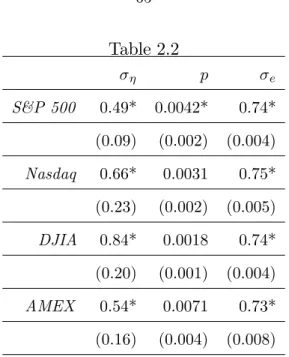
2.2 Maximum Likelihood Estimates of the Basic RLS Model . . . 65
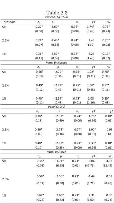
2.3 Maximum Likelihood Estimates of RLS Model with time varying Proba-bility . . . 66
2.4 Maximum Likelihood Estimates of the RLS Model with Mean Reversion 67 2.5 Maximum Likelihood Estimates of RLS Model with a time varying Proba-bility of shifts and Mean Reversion . . . 68
2.6 Out-of-Sample Forecast Compariosn . . . 69
3.1 Finite sample size of the t-statistics for meant^ 1 using ELW . . . 90
3.2.2 Finite sample size of the t-statistics for trend slope t^
2 using ELW . . . 92
3.3 Finite sample size of the t-statistics for mean and trend slope . . . 93
3.4 Finite sample size comparisons . . . 94
3.5 Empirical applications to temperature series . . . 95
1.1 Particle Filtered Estimates and Trues Values of the Parameter Process . 40
1.2 Particle Filtered Estimates and True Values of the Parameter and
Sto-chastic Volatility Processes . . . 41
1.3 Out-of-Sample Forecasts of the Equity Premium . . . 42-43 1.4 Out-of-Sample Forecasts of In‡ation . . . 44
2.1 Full Sample autocorrelations . . . 70
2.2 Fitted level shifts and volatility . . . 71
2.3 Sample autocorrelations of S&P 500 residuals . . . 72
2.4 S&P500 Smoothed …lter of the level shifts for di¤erent thresholds . . . 73
2.5 S&P Smoothed …lter of the level shift components for di¤erent models . 74 2.6 Autocorrelation function of the residual term in RLS with both mean reversion and changing probability . . . 75
3.1 Finite sample power of the t-statistic for mean t^ 1 (T=500) . . . 96
3.2 Finite sample power of the t-statistics for trend slope t^ 2 (T=500) . . . 97
3.3 Finite sample power of the t-statistic for mean t^ 1 (T=1000) . . . 98
3.4 Finite sample power of the t-statistic for trend slopet^ 2 (T=1000) . . . 99
3.6 Temperature series . . . 101
AIC Akaike Information Criterion
AMO Atlantic Multidecanal Oscillation
ARFIMA Autoregressive Fractional Integration Moving Average
DGP Data Generating Process
DJIA Dow Jones Industrial Average
ELW Exact Local Whittle
EM Expectation Maximization
ESS E¤ective Sample Size
GLS Genenralized Least Square
LSV Long Memory Stochastic Volatility
MCEM Monte Carlo Expectation Maximization
MCMC Markov Chain Monte Carlo
MCS Model Con…dence Set
MSFE Mean Square Forecast Error
MU Median Unbiased
RLS Random Level Shift
SIR sampling/importance resampling
SIS sequential importance sampling
SISR sequential importance sampling with resampling
UB Upper Biased
UC-SV Unobserved Component Stochastic Volatility
UIRP Uncovered Interest Rate Parity
Chapter 1
A new approach to forecasting in the presence of
in and out of sample breaks
1.1 Introduction
Forecasting is obviously of paramount importance in time series analyses. The theory of constructing and evaluating forecasting models is well established in the case of stable relationships. However, there is growing evidence that forecasting models are subject to instabilities, leading to imprecise and unreliable forecasts. This is so in a variety of …elds including macroeconomics and …nance. Indeed, Stock and Watson (1996) documented wide-spread prevalence of instabilities in macroeconomic time series relationships. A prominent example is forecasting in‡ation; see, e.g., Stock and Watson (2007). This problem is also prevalent in …nance. Pastor and Stambaugh (2001) document structural breaks in the con-ditional mean of the equity premium using long time return series. Paye and Timmermann (2006) examined model instability in the coe¢ cients of ex post predictable components of stock returns. See also Pesaran and Timmermann (2002), Rapach and Wohar (2006) and Pettenuzzo and Timmermann (2011).
There is a vast literature on testing for and estimating structural changes within a given sample of data; see, e.g., Andrews (1993), Bai and Perron (1998, 2003) and Perron (2006) for a survey. Much of the literature does not model the breaks as being stochastic. Hence, the scope for improving forecasts is limited. There can be improvements by relying on the estimates of the last regime (or at least putting more weights on them) but even then such improvements are possible if there are no sample breaks. In the presence of out-of-sample breaks the limitation imposed by treating the breaks as deterministic mitigates the
forecasting ability of models corrected for in-sample breaks. This renders forecasting in the presence of structural breaks quite a challenge; see, e.g., Clements and Hendry (2006).
Some Bayesian models have been proposed to address this problem; see, e.g., Pesaran et al. (2006), Koop and Porter (2007), Maheu and Gordon (2008), Maheu and McCurdy (2009) and Hauwe et al. (2011). The advantage of the Bayesian approach steams from the fact that it treats the parameters as random and by imposing a prior (or meta-prior) distribution one can model the breaks and allow them to occur out-of-sample with some probability. Such methods can, however, be sensitive to the exact prior distributions used. We propose a frequentist-type approach with a forecasting model in which the changes in the parameters have a probabilistic structure so that the estimates can help forecast future out-of-sample breaks. Our approach is best suited to the case for which breaks occur both in and out-of-sample, which in particular avoids the problematic use of a trimming window assumed to have a stable structure. The method will work best indeed if there are many in-sample breaks, so that a long span of data is bene…cial. This is unavoidable since good out-of-sample forecasts of breaks require in-sample information about the process generating such breaks, the more so the more e¢ cient the forecasts will be. The same applies to previously proposed Bayesian methods, though the use of tight priors can partially substitute for the lack of precise in-sample information. Having said that, our method still yields considerable improvements even if relatively few breaks are present in-sample.
Our approach is similar in spirit to unobserved components models in which the para-meters are modeled as random walk processes. There are, however, important departures. Most importantly, a shift need not occur every period. It does so with some probability dictated by a Bernoulli process for the occurrence of shifts and a normal random variable for its magnitude. This leads to a speci…cation in which the parameters evolve according to a random level shift process. Some or all of the parameters of the model can be allowed to change and the latent variables that dictate the changes can be common or di¤erent for each parameters. Also, the variance of the errors may change in a similar manner.
mean of a time series, whether stationary or long-memory, in particular to try to assess whether a seemingly long-memory model is actually a random level shift process or a genuine long-memory one; see Ray and Tsay (2002), Perron and Qu (2010), Lu and Perron (2010), Qu and Perron (2012), Varneskov and Perron (2012), Li and Perron (2012) and Xu and Perron (2012). It has been shown to provide improved forecasts over commonly used short or long-memory models. Our basic framework is a generalization in which any or all parameters of a forecasting model are modeled as random level shift processes.
To improve the forecasting performance we augment the model in two directions. First, we model the probability of shifts as a function of some covariates which can be forecasted. Second, we allow a mean-reversion mechanism such that the parameters tend to revert back to the pre-forecast average. This last feature is especially in‡uential in providing improvements in forecasting performance at long horizons. Functional forms for these two modi…cations are suggested for which the parameters can be estimated and incorporated in the forecast scheme to model the future path of the parameters.
Our model can be cast into a non-linear non-Gaussian state space framework for which standard Kalman …lter type algorithms cannot be used. The state space representation of our model is actually a linear dynamic mixture models in the sense that it is linear and Gaussian conditional on some latent random variables. See Giordani et al. (2007) who discuss the advantages of the class of conditionally linear and Gaussian state space models. To provide a computationally e¢ cient method of estimation, we rely on recent developments on particle …ltering methods. The predictive distribution of the state is approximated by a weighted sum of particles. The key to particle …ltering is turning integrals into sums via discrete approximations. The EM algorithm is used to obtain the maximum likelihood estimates of the parameters. This allows treating the latent state variables as missing data (see Bilmes, 1998) and using a complete or data-augmented likelihood function which is easier to evaluate than the original likelihood. Since the missing information is random, the complete-data likelihood function is a random variable and we end up maximizing the expectation of the complete-data log-likelihood with respect to the missing data. Wei and
Tanner (1990) introduced the Monte Carlo EM algorithm where the evaluation step is executed by Monte Carlo methods. Random samples from the conditional distribution of the missing data (state variables) can be obtained via a particle smoothing algorithm. For an application of the use of such methods to the estimation of stochastic volatility models, see Kim (2006). The forecasting procedure is then relatively simple and can be carried out in a straightforward fashion once the model has been estimated. Simulations show that the estimation method provides very reliable results in …nite samples. The parameters are estimated precisely and the …ltered estimates of the time path of the parameters follow closely the true process.
We apply our forecasting model to a variety of series which have been the object of considerable attention from a forecasting point of view. These include the equity premium, in‡ation, exchange rates and the Treasury bill interest rates. In each case, we compare the forecast accuracy of our model relative to the most important forecasting methods applicable for each variable. We also consider di¤erent forecasting sub-samples or periods. The results show clear gains in forecasting accuracy, sometimes by a very wide margin; e.g., over 80% reduction in mean squared forecast error for the equity premium over all popular contenders.
Finally, note that given the availability of the proper code for estimation and forecasting, the method is very ‡exible and easy to implement. For a given forecasting model, all that is required by the users are: 1) which parameters (including the variance of the errors if desired) are subject to change; 2) whether the same or di¤erent latent Bernoulli processes dictates the timing of the changes in each parameters; 3) which covariates are potential explanatory variables to model the probability of shifts.
The rest of the paper is organized as follows. Section 2 describes the basic model with random level shifts in the parameters. Section 3 discusses the modi…cations introduced to improve forecasting: the modeling of the probability of shifts and the allowance for a mean-reverting mechanism. Section 4 presents the estimation methodology: the particle …ltering algorithm in Section 4.1, the particle smoothing algorithm in Section 4.2, the Monte Carlo
Expectation Maximization method to evaluate the likelihood function in Section 4.3, and in Section 4.4 issues related to initialization and the construction of the standard errors of the estimates. Section 5 presents results pertaining to the accuracy of the estimation method in …nite samples. Section 6 contains the various applications and comparisons with other forecasting methods. Section 7 o¤ers brief concluding remarks.
1.2 The basic model
We consider a basic forecasting model speci…ed by
yt=Xt t+et (1.1)
whereytis a scalar variable to be forecasted,Xtis a k-vector of covariates and, in the base case et i:i:d: N(0; 2e). It is assumed that the some or all of the parameters are time-varying and exhibit structural changes at some unknown time. The speci…cation adopted for the time-variation in the parameters is the following:
t= t 1+Kt t
where Kt = diag(K1;t; :::; Kk;t) and t = ( 1;t; :::; k;t)0 i:i:d: N(0; ). The latent vari-ablesKj;t Ber(p(j))and are independent acrossj. Hence, the parameter evolves according to a Random Level Shift (RLS) process such that the shifts are dictated by the outcomes of the Bernoulli random variables Kj;t. When Kj;t = 1, a shift j;t occurs drawn from a
N(0; 2;j)distribution, otherwise whenKj;t = 0, the parameter does not change. The shifts can be rare (small values ofp(j)) or frequent (larger values ofp(j)).
This speci…cation is ideally suited to model changes in the parameters occurring at unknown dates. Many speci…cations are possible depending on the assumptions imposed onKt and . First, when K1;t =:::=Kk;t, we can interpret the model as one in which all parameters are subject to change at the same times, akin to the pure structural change model of Bai and Perron (1998). A partial structural model, can be obtained by setting p(j) = 0
and columns of to0. The case withK1;t =:::=Kk;t is arguably the most interesting for a variety of applications. However, it is also possible not to impose equality for the di¤erent
Kj;t. This allows the timing of the changes in the di¤erent parameters to be governed by di¤erent independent latent processes. This may be desirable in some cases. For instance, it is reasonable to expect changes in the constant to be related to low frequency variations of the random level shifts type, while changes in the coe¢ cients associated with random regressors to be related to business-cycle type variations. In such cases, it would therefore be desirable to allow the timing of the changes to be di¤erent for the constant and the other parameters. Of course, many di¤erent speci…cations are possible, and the exact structure needs to be tailored to the speci…c application under study.
The assumption that the latent Bernoulli processes Kj;t are independent acrossj may seem strong. It implies that the timing of the changes are independent across parameters. As stated above, this can be relaxed by imposing a perfect correlation, i.e., setting some latent variables to be the same. Ideally, one may wish to have a more ‡exible structure that would allow imperfect though non-zero correlation. This generalization is not feasible in our framework. In many cases, it may also be sensible to impose that is a diagonal matrix. This implies that the magnitudes of the changes in the various parameters are independent. In our applications, we follow this approach as it appears the most relevant case in practice and also considerably reduces the complexity of the estimation algorithm to be discussed in the next section. Hence, for thejth parameter j (j= 1; :::; k), we have
j;t= j;t 1+Kj;t j;t (1.2)
where j;t N(0; 2;j) and Kj;t Ber(p(j)).
In some cases, it may also be of interest to allow for changes in the variance of the errors. The speci…cation for the distribution is thenet= ";t"t with
ln 2";t = ln 2";t 1+Ktv";t (1.3)
Remark 1 When p(j)=p = 0 for allj, the model reduces to the classic regression model
with time invariant parameters. Whenp(j)= 1 for allj andp = 0, it becomes the standard
time varying parameter model; e.g., Rosenberg (1973), Chow (1984), Nicholls and Pagan (1985) and Harvey (2006).
Remark 2 The model can be extended to a multiple regressions framework such as VAR models. However, the focus here will be on a single equation model.
1.3 Modi…cations useful for forecasting improvements
The framework laid out in the previous section is well tailored to model in-sample breaks in the parameters. However, as such it does not allow future breaks to play a role in forecasting. In order to be able to do so, we incorporate some modi…cations. Two features that are likely to improve the …t and the forecasting performance is to allow for changes in the probability of shifts and model explicitly a mean-reverting mechanism for the level shift component. In the …rst step, we specify the jump probability to be
p(j)t =f(p; wt)
where p is a constant,wt are covariates that would allow to better predict the probability of shifts and f is a function that ensure that pt 2[0;1]. Note that wt needs to be in the information set at timetin order for the model to be useful for forecasting. We shall adopt a linear speci…cation with the standard normal cumulative distribution function ( ), so that Kj;t Ber(pt) with pt= (r0+r1wt). As similar speci…cation can be made for the probability of the Bernoulli random variable Kt a¤ecting the shifts in the variance of the errors.
The second step involves building a mean reverting mechanism to the level shift model. The motivation for doing so is that we observe evidence that parameters does not jump arbitrarily and that large upward movement tend to be followed by a decrease. This fea-ture can be bene…cial to improve the forecasting performance if explicitly modeled. The
speci…cation we adopt is the following:
j;t N( ;j;t; 2;j) ;j;t = ( j;t 1
(t 1)
j )
where j;t 1 is the …ltered estimate of the parameter subject to change at time t 1 and (t 1)
j is the mean of all the …ltered estimates of the jump component from the beginning of the sample up to timet 1. This implies a mean-reverting mechanism provided <0. The magnitude of then dictates the speed of reversion. Note that the speci…cation involves using data only up to time t 1in order to be useful for forecasting purposes. Also, it will have an impact on forecasts since being in a high (low) values state implies that in future periods the values will be lower (higher), and more so as the forecasting horizon increases. Hence, this speci…cation has an e¤ect on the forecasts of both the sign and size of future jumps in the parameters. Similar speci…cations can be made top and v";t for the changes in the variance of the errors.
The out-of-sample forecasts are then constructed in two steps. The …rst involves fore-casting the covariateswtusing a preliminary model; e.g., using anAR(p). Theh-step ahead forecast of the jump probability is thenpt+hjt= (r0+r1wt+hjt)wherewt+hjt is theh-step ahead forecast ofwt+h at timet. Note that one can also forecast the regressorsXtto obtain predicted values denoted byXt+hjt. The second step is to forecast j;t as a weighted sum of two di¤erent possible outcomes: one with structural breaks and one without. For example, the one-step-ahead forecast at time tis
j;t+1jt=E( j;t+1j j;t) = (1 p (j)
t+1jt) j;t+p (j)
t+1jt( j;t+ ;j;t+1jt);
to compute future conditional means. Therefore, the h-step ahead forecast is j;t+hjt = E( j;t+hj j;t) =E( j;t+ h X k=1 p(j)t+kjt ;j;t+kjtj j;t) = j;t+ h X k=1 pt+kjt ;j;t+kjt= j;t+ h X k=1 p(j)t+kjt ( j;t+k 1jt (t+kj 1))
As the forecast horizon increases, the probability of future structural changes also increases. This feature is also present in some Bayesian-type forecasting methods for out-of-sample structural breaks; see, e.g., Hauwe et al. (2011).
1.4 Estimation Methodology
The model described is within the class of non-linear non-Gaussian State Space models of the form
yt = Ht(xt; vt) xt = Ft(xt 1; ut)
whereyt is the variable to be forecasted andxt are the latent processes. The measurement equation is (1.1) and the transition equations are (1.2) and (1.3). This implies that standard Kalman …lter type algorithms are not appropriate and that an extended estimation method is needed. The one adopted is discussed in this section.
1.4.1 Particle …ltering
As an alternative to simulation-based algorithms like Markov Chain Monte Carlo (MCMC) methods, particle …lters and smoothers are sequential Monte Carlo methods used to eval-uate the probability distribution of some variable x, which is hard to compute directly as in cases for which the analytic solutions are not available. They approximate the contin-uous distribution of x by a discrete distribution involving a set of weights and particles fw(i); x(i)gMi=1. We can view particle …lters and smoothers as generalizations of the Kalman …lters and smoothers for general state space models. Since our model setup includes
mix-tures of normal errors and stochastic volatility, standard Kalman …ltering and smoothing techniques are not applicable. Of particular interest is the fact that sequential Monte Carlo …ltering or particle …ltering enables us to approximate the conditional densityf(xtjy(t))as a weighted sum of particles, where y(t) = (y
1; :::; yt) denotes the history of the data up to timet.
The …ltered distribution of xt+1 conditional on information up to time t+ 1is
p(xt+1jy(t+1))/p(yt+1jxt+1)p(xt+1jy(t)) (1.4)
The likelihoodp(yt+1jxt+1)is usually known, and the predicting densityp(xt+1jy(t))is given by:
p(xt+1jy(t)) = Z
p(xt+1jxt)p(xtjy(t))dxt (1.5) Particle …ltering methods approach the …ltering problem through simulations and a dis-crete approximation of the optimal …ltering distribution. More precisely, particle methods approximate p(xtjy(t)) by pM(xtjy(t)) = M X i=1 !(i)t x(ti)
where is the Dirac delta function andf!(i)t ; x(i)t gMi=1 denote a set of weights and particles. HereM is the number of particles. See Johannes and Polson (2006) for a brief introduction to particle …ltering, and Doucet et al. (2001) and Ristic et al. (2004) for a textbook discussion. For applications to stochastic volatility models using particle …ltering, see Kim et al. (1998), Chib et al. (2006) and Malik and Pitt (2009). Pitt (2005) applies particle …ltering to maximum likelihood estimation, while Fernandez and Rubio (2005) apply it to dynamic macroeconomic models. See also Creal (2012) for a survey of applications of sequential Monte Carlo methods in economics and …nance.
Via resamplingfw(i)t ; x(i)t gi=1M can yield an equally weighted random sample fromp(xtjy(t)). Therefore, we can discretely approximate p(xtjy(t)) by
pM(xtjy(t)) = 1 M M X i=1 p(ytjxt)p(xtjx(i)t 1):
Hence, using (1.5) we can update p(xtjy(t)) to p(xt+1jy(t)), and using (1.4) we can obtain sample particles from p(xt+1jy(t+1)). There are di¤erent sampling strategies developed in the literature, such as sampling/importance resampling (SIR), sequential importance sam-pling (SIS), exact particle …ltering and auxiliary particle …ltering algorithms. We adopt the sequential importance sampling with resampling (SISR) algorithm to get particles from p(xt+1jy(t+1)). This algorithm was introduced by Gordon et al. (1993) to add a resampling step within the SIS algorithm that can mitigate the weight degeneracy problem. A sequen-tial importance density q(xt+1jy(t+1)) is introduced, which is easier to sample from than p(xt+1jy(t+1)):By the change of measure formula
E[f(xt+1)jy(t+1)] =
Eq[wt+1f(xt+1)jy(t+1)] Eq[wt+1jy(t+1)]
;
withwt=p(xtjy(t))=q(xtjy(t)). Given samples from the importance density,
EM[f(xt+1)jy(t+1)]/ M X i=1
w(i)t+1f(x(i)t+1)
Given the recursive speci…cations for p(xt+1jy(t+1)) andq(xt+1jy(t+1)), we have
p(xt+1jy(t+1))/p(yt+1jxt+1)p(xt+1jxt)p(xtjy(t))
and
q(xt+1jy(t+1))/q(xt+1jxt; y(t+1))q(xtjy(t)) The weights are also recursive, so that:
w(i)t+1 = p(x (i) t+1jy(t+1)) q(x(i)t+1jy(t+1)) = p(yt+1jx(i)t+1)p(x (i) t+1jx (i) t ) q(x(i)t+1jx(i)t ; y(t+1)) p(x(i)t jy(t)) q(x(i)t jy(t)) = p(yt+1jx (i) t+1)p(x (i) t+1jx (i) t ) q(x(i)t+1jx(i)t ; y(t+1)) w (i) t
The …rst equation follows from the de…nition of the change of probability measures, and the second from the recursive representation for p(xt+1jy(t+1)) and q(xt+1jy(t+1)). We
summa-rize the steps involved in implementing the SISR algorithm in the context of our forecasting model with one parameter subject to change and no stochastic volatility, in which case the state or latent variables arefKtgand j;t.
Particle …ltering algorithm based on SISR: First, for i = 1; : : : ; M: generate
K0(i) Ber(p0), then (i)0 K0(i) N( 0; 20). Set the initial weights to w0(i) =
(1=M). Second, fort= 1; : : : ; T: generate Kt(i) Ber(pt) and (i)t = (i) t 1+K (i) t N( ;t; 2), compute wt(i)/p(ytjx(i)t )w (i) t 1/ 1 p 2 2 e exp( (yt Xt (i) t )2 2 2 e );
for i = 1; : : : ; M, and normalize the weights to get w^(i)t = wt(i)=PMi=1wt(i). Then, resample f (i)t ; Kt(i)gMi=1 with probability w^(i)t , and set w(i)t = (1=M). Repeat the steps above increasing fromt+ 1until T.
Remark 3 Resampling the particlesf (i)t ; Kt(i)gMi=1 implies replicating a new population of particles from the existing population in proportion to their normalized importance weights.
In Gordon et al. (1993), resampling is carried out every time period, and M random
variables are drawn with replacement from a multinomial distribution with probabilities fw^(i)t gM
i=1. After resampling, we set the weights of the particles to a constant (1=M). This
resampling scheme allows solving the weight degeneracy problem of the SIS algorithm. Remark 4 Liu and Chen (1995) suggest to resample only when the importance weights are unstable to decrease the e¤ ect of Monte Carlo variation impacted to the estimator. The e¤ ective sample size (ESS) as a measure of the weight instability is de…ned as:
ESS = PM 1
i=1( ^w (i) t )2
At each time period, ESS is calculated and compared to a user chosen threshold. If ESS drops below the threshold, then resampling is performed. Usually the threshold is picked as a percentage of the number of particles, e.g., in the range 0.5 to 0.75. In our applications, we use 0.5.
1.4.2 Particle Smoothing
The particle smoothing algorithm is designed to obtain particle smothers fs(i)t gMi=1 with certain weights fwt(i)gM
i=1 from p(xtjy(T)). Godsill et al. (2004) provide a forward-…ltering and backward-simulation smoothing procedure. It allows drawing random samples from the joint densityp(x0; x1; : : : xTjy(T)), not only the individual marginal smoothing densities p(xtjy(T)):The smoothing algorithm relies on a pre-…ltering procedure and previously ob-tained set of particlesfwt(i); x(i)t gMi=1 for each time period. The main ingredients behind the smoothing algorithm are the relations:
p(x1; x2; : : : ; xTjy(T)) =p(xTjy(T)) TY1 t=1 p(xtjxt+1; : : : ; xT; y(T)) and p(xtjxt+1; : : : ; xT; y(T)) = p(xtjxt+1; y(t)) = p(xtjy (t))p(x t+1jxt) p(xt+1jy(t)) / p(xtjy(t))p(xt+1jxt)
The …rst equality follows from the Markov property of the model and the second from Bayes’rule. Since random samplesfx(i)t gMi=1fromp(xtjy(t))can be obtained from the particle …ltering algorithm,p(xtjxt+1; : : : ; xT; y(T))can be approximated asPMi=1w
(i) tjt+1 x(ti)(xt)with modi…ed weights wt(i)jt+1 = w (i) t p(xt+1jx(i)t ) PM i=1w (i) t p(xt+1jx(i)t ) :
This procedure is performed in a reverse-time direction conditioning on future states. Given a random samplefst+1; : : : ; sTgdrawn fromp(xt+1; : : : ; xTjy(T)), we take one step back and sample st from p(xtjst+1; : : : ; sT; y(T)). The smoothing algorithm is summarized as follows in the context of the simple version of our model.
Particle smoothing algorithm: Consider the weighted particles obtained from the …ltering algorithm fw(i)t ; (i)t ; Kt(i)gMi=1 for i = 1; : : : ; M, and t = 1; : : : ; T. Let fs(j);t; s(j)K
1;tg M
j=1 be a set of particle smoothers. First set s (j) ;T = (i) T ands (j) K1;T =K (i) T
with probability (1=M). Then, fort=T 1; T 2; : : : ;1, compute
w(i)tjt+1 / w(i)t p(s(j);t+1j (i)t )
/ fpt+1exp( (s(j);t+1 (i)t ;t)2 2 2 )g s(Kj) 1;t+1f1 pt+1g1 s (j) K1;t+1
for i = 1; : : : ; M, and let s(j);t = (i)t and s(j)K
1;t+1 = K (i)
t with probability w
(i) tjt+1. Repeat the steps above decreasing from t 1 until 1 to obtain fs(j);t; s(j)
Kt;t+1g as approximations top( t; Ktjy(T)), forj= 1; : : : ; M.
1.4.3 MCEM algorithm
Frequentist likelihood-based parameter estimation of non-linear and non-Gaussian state space models using particle …lters and smoothers is not straightforward. The gradient-based optimizer su¤ers from a discontinuity problem caused by the resampling. Here, we follow the Monte Carlo Expectation Maximization (MCEM) method proposed by Olsson et al. (2008). The Basic EM algorithm is a general method to obtain the maximum-likelihood estimates of the parameters of an underlying distribution from a given data set with missing values. Suppose the complete data set is Z = (Y; X), in which Y is observed butX is unobserved. For the joint densityp(zj ) =p(y; xj ) =p(yj )p(xjy; ), we de…ne the complete-data likelihood function by L( jY; X) = p(Y; Xj ). The original likelihood
L( jY)is the incomplete-data likelihood. SinceXis unobserved and may be generated from an underlying distribution, e.g., the transition equation in a state space model,L( jY; X)
is indeed a random variable. Therefore, we maximize the expectation oflogL( jY; X)with respect toX, with the expectation de…ned by:
Q( ; (k 1)) =E[logL( jY; X)jY; (k 1)] =
Z
logp(Y; xj )p(xjY; (k 1))dx
The di¤erence between Monte Carlo EM algorithm and the basic EM algorithm is that when evaluating Q( ; (k 1)), the MCEM uses a Monte-Carlo based sample average to
approximate the expectation. The Monte Carlo Expectation or E-step is: Q ( ; (k 1)) = 1 M M X i=1 logp(Y; x(i)j )
where fx(i)gMi=1 are random samples from p(xjY; (k 1)). Given current parameter esti-mates, random samples from p(xjY; (k 1)) are simply the particle smoothers fs(i)
t gMi=1 obtained as described above. The Maximization or M-step is:
(k)= arg maxQ( ; (k 1))
These two steps are repeated until (k)converges. The rate of convergence has been studied by many researchers; e.g., Dempster et al. (1977), Wu (1983) and Xu and Jordan (1996). In the context of the simple version of our model, the speci…cs of the algorithm are as follows. For the E-step, the complete likelihood of f 1; : : : ; T; K1; : : : ; KT; y1; : : : ; yTg is
f( ; K1; Y) = T Y t=1 f( tj t 1; Kt) T Y t=1 f(Kt) T Y t=1 f(ytj t; Kt) = f T Y t=1 1 q 2 2exp( ( t t 1 ;t)2 2 2 )g Kt T Y t=1 pKt t (1 pt)1 Kt T Y t=1 1 p 2 2 e exp( (yt Xt t) 2 2 2 e )
The log-likelihood function is:
2logf( ; K ; Y) = T X t=1 Kt[log( 2) +( t t 1 ;t) 2 2 ] 2 T X t=1 [Ktlog(pt) + (1 Kt)log(1 pt)] + T X t=1 [log( 2e) +(yt Xt t) 2 2 e ]
The expectation of the complete log-likelihood function with respect to the unknown state variables ; K given Y and current parameter estimates (k 1) is the objective function to be maximized (or minimized if using the negative of the log-likelihood function). For the Monte Carlo EM algorithm, we approximate the expectation by Monte Carlo sample aver-age with random samples drawn fromp( t; KtjyT) obtained using the particle smoothing algorithm. Then, Q( ; (k 1)) = E[ 2logf( ; K ; Y)jY; (k 1)] = 1 M M X i=1 f T X t=1 Kt(i)[log( 2) +( (i) t (i) t 1 (i) ;t)2 2 ] 2 T X t=1 [Kt(i)log(pt) + (1 K (i) t )log(1 pt)] + T X t=1 [log( 2e) +(yt Xt (i) t )2 2 e ]g
For the M-step, note that conditional on K , the model is a linear Gaussian state space model. Hence, standard maximum likelihood estimates are obtained by solving the …rst order condition.
Remark 5 For the full model with stochastic volatility, the estimation methodology is the same. The di¤ erence is that instead of having two state variables, we now have four state
variables f t; Kt; ln 2";t; Ktg. Similarly, if di¤ erent parameters are allowed to vary
inde-pendently, we simply add the additional latent variables ( jt; Kjt).
1.4.4 Selection of the initial values and construction of the standard errors In order to speed up the convergence of the estimation algorithm, we can use information from the data in order to provide better initial parameter values. Consider for example, the simple model
yt = t+et t = t 1+Kt t
where t N(0; 2),et N(0; 2e) and Kt Ber(p). The initial parameter values are set top(0) 2(0) =jvar(y y 2) var(y y 1)jand 2 (0) e = (var(y y 1) p(0) 2 (0) )=2. We set
p(0) according to prior judgment about the frequency of the jumps.
To construct the standard errors of the estimates, Louis (1982) provides a way of ob-taining the information matrix when using the EM algorithm. It is given by
I = T X t=1 E[B( t;^ )j t] T X t=1 E[S( t;^ )ST( t;^ )j ] 2 T X t<k E[S( t;^ )j ]E[S( k;^ )j ]0
where S( t;^ ) and B( t;^ ) are the …rst and second order derivatives, respectively and refers to the complete data set including both observed data and unobserved state variables. However, since simulations are used in the EM algorithm, this may cause discontinuities, in which case this method is unstable and cannot always provide a positive de…nite covariance matrix. Duan and Fulop (2011) proposed a stable estimator of the information matrix applicable to the EM algorithm. They estimate the variance using the smoothed individual scores. De…neat( ) =E[@logf(xtj t 1; )=@ jY; ], then the estimate of the information matrix is ^ I = 0+ l X j=1 w(l)( j+ 0j)
where j =PTt 1jat( ^ )at+j( ^ )0 and w(j) = 1 j=(l+ 1). This method is easy to compute and does not require evaluations of the second-order derivatives of the complete data log-likelihood.
1.5 Simulations
We now present simulation results to assess the adequacy of our estimation method in providing good estimates in …nite samples. All simulation results are obtained from N = 1000particles and the sample size is T = 1000. The number of replications is 500.
the variance of the errors does not change. The model is then
yt = t+et (1.6)
t = t 1+Kt t
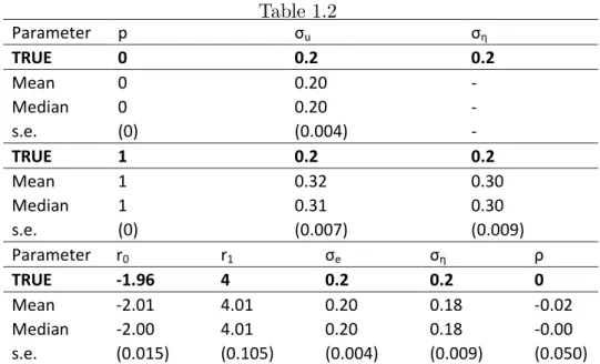
where et i:i:d: N(0; 2e), t i:i:d: N(0; 2) and Kt Ber(pt) withpt= (r0+r1wt). We start with a case with infrequent shifts with parameters given by 0 = (r0; r1; e; ) =
( 1:96;4;0:2;0:2). Since we are not concerned about forecasting here, we set ;t = 0. The covariate wt is a vector in which every 50 time periods wt = 1, and 0 otherwise. Hence, a shift occurs with probability very close to one every 50 periods, otherwise the probability of a shift is 2.5%. We also consider a case with frequent jumps so that a shift occurs with probability0:5every time period. In this case the parameter values are 0= (0;0;0:2;0:2). In both cases, we use the true parameter values as the initial conditions. Table 1 (panel A) presents the mean and standard errors of the estimates showing that, in both cases, they are very accurate. Figure 1(a,b) presents a plot of the true path of the process t along with the …ltered estimates tjt obtained for the particle …lter algorithm. This is done for a single realization chosen randomly. These reveal that the …ltered estimates provide very accurate estimates of the time path of the parameter.
We now present results when using adding a mean reverting component and allowing the variance of the errors to change. Hence,et= ";t"t with
ln 2";t = ln 2";t 1+Ktv";t (1.7)
where"t i:i:d: N(0;1),Kt Ber(p )andv";t i:i:d: N(0; 2v). Also,
t N( ;t; 2)
;t = ( t 1
(t 1)
)
The true parameters are 0 = (r0; r1; p ; ; v; ; ) = ( 1:96;4;0:5;0:95;0:2;0:2; 0:1). The covariatewtis as speci…ed before. The mean and standard deviations of the estimates
are presented in Panel B of Table 1. Figure 2 presents a graph of the path of the true t andln 2
";talong with their …ltered estimates, again for a single realization chosen randomly. The results show that the mean values of the estimates are close to the true values. The …ltered estimates of t and ln 2
";t follow the general time variations of the true processes, though not as precisely as in the simpli…ed case.
To assess the robustness of our estimation method, we …rst consider the simpli…ed model (1.6) withKt Ber(p) for two extreme cases involving a constant probability of changes. One has tconstant (jump probability0) and the other has tchanging every period (jump probability 1). Here, the parameter space of interest is = (p; e; ). The simulation results for the means and standard deviations are presented in Table 2 for both cases. For the case with p = 0, the estimates are very accurate. When p = 1, p is very precisely estimated but the estimates of e and are slightly biased upward.
The next experiment aims to assess whether it is detrimental to introduce a mean reversion component when none is present. To that e¤ect, we use model (1.6) with the addition that
t N( ;t; 2)
;t = ( t 1
(t 1)
)
The true parameter values are 0 = (r0; r1; e; ; ) = ( 1:96;4;0:2;0:2;0). The results presented in the last panel of Table 2 show that the estimate of all parameters are precise so that no e¢ ciency loss is incurred.
1.6 Forecasting applications
We consider a variety of forecasting applications pertaining to variables which have been the object of intense attention in the literature: the equity premium, in‡ation, the treasury bill rate and exchange rates. We compare the forecasting performance of our model relative to popular forecasting methods applicable to the di¤erent variables. In all cases, our model provides improved forecasts, in some cases by a considerable margin.
Throughout, the out-of-sample forecasting experiments aim at evaluating the experience of a real-time forecaster by performing all model speci…cations and estimations using data through date t, making a h-step ahead forecast for date t+h, then moving forward to datet+ 1and repeating this through the sub-sample used to construct the forecasts. The estimation of each model is recursive, using an increasing data window starting with the same initial observation. The forecasting performance is evaluated using the mean square forecast error (MSFE) criterion de…ned as
M SF E(h) = 1 Tout Tout X t=1 (yt;h yt+hjt)2
whereToutis the number of forecasts produced,his the forecasting horizon,yt;h=Phk=1yt+k and yt+hjt=
Ph
k=1yt+kjt withyt+k the actual observation at timet+k and yt+kjt its fore-cast conditional at time t. To ease presentation, the MSFE are reported relative to some benchmark model, usually the most popular forecasting model in the literature. In all cases, we allow mean reversion in the paramters of the model when constructing forecasts using our model.
1.6.1 Equity premium
Forecasts of excess returns at both short and long-horizons are important for many economic decisions. Much of the existing literature has focused on the conditional return dynamics and studied the implications of structural breaks in regression coe¢ cients including the lagged dividend yield, short interest rate, term spread and the default premium. However, most of the research has focused on modeling the equity premium assuming a certain num-ber of structural breaks in-sample while ignoring potential out-of-sample structural breaks. Recently, Maheu and McCurdy (2009) studied the e¤ect of structural breaks on forecasts of the unconditional distribution of returns, focusing on the long-run unconditional distrib-ution in order to avoid model misspeci…cation problems. Their empirical evidence strongly rejects ignoring structural breaks for out-of-sample forecasting. We consider using our fore-casting model with di¤erent speci…cations. One models the unconditional mean of excess
returns incorporating random level shifts in mean, with the time varying jump probabilities in‡uenced by the absolute rate of growth in the earning price ratio. We also consider a conditional mean model using the dividend yield as the explanatory variable.
Following Jagannathan et al. (2000), we approximate the equity premium of S&P 500 returns as the di¤erence between stock yield and bond yield. The data were obtained from Robert Shiller’s website (http://www.econ.yale.edu/~shiller/data.htm). According to Gordon’s valuation model, stock returns are the sum of the dividend yields and the expected future growth rate in stock dividends. We use the average dividend growth rate to proxy for the expected future growth rate. The data is monthly and covers the period from 1871 to 2012.5. High quality monthly data are available after 1927, before 1927 the monthly data are interpolated from lower frequency data. We use the 10-year Treasury constant maturity rate (GS10) as the risk free rate.
We start with a simple random level shift model without explanatory variables given by:
yt = t+et (1.8)
t = t 1+Kt t whereet i:i:d: N(0; 2e), t i:i:d: N( ;t; 2), ;t= ( t 1
(t 1)
),Kt Ber(pt)withpt
= (r0+r1wt). The covariate wt used to model the time variation in the probability of shifts is the lagged absolute value of the rates of changes in the EP ratio. The rational for doing so that it is expected that large ‡uctuations in the earning price ratio induce a higher probability that excess stock returns will experience a level shift in the unconditional mean. We also allow a mean reversion component and to assess its e¤ect we also consider a version without it. To implement the forecasts, we use anAR(p)model to forecastwtfor which, here and throughout all applications, the number of lags is selected using the Akaike Information Criterion (AIC) with a maximal value of 4.
ratio as the regressor. The speci…cations are
yt= 1t+ 2tdpt 1+et (1.9)
where, with t= ( 1t; 2t),
t= t 1+Kt t:
Lettau and van Nieuwerburgh (2007) analyzed the implications of structural breaks in the mean of the dividend price ratio for conditional return predictability. Xia (2001) studied model instability using a continuous time model relating excess stock returns to dividend yields. They model the coe¢ cient t to follow an Ornstein–Uhlenbeck process and the ensuing estimates of the time varying coe¢ cient 2t revealed instability of the forecasting relationship. Hence, instabilities have been shown to be of concern when using this con-ditional forecasting model, which motivates the use of our forecasting model. Besides the addition of the lagged dividend price ratio as regressors, the speci…cations are the same as for the unconditional mean model (1.8).
We consider various versions depending on which coe¢ cients are allowed to change and if so whether they change at the same time. These are: 1) the unconditional mean model (1.8) with level shifts, 2) the conditional mean model (1.9) with the coe¢ cient on the lagged dividend yield allowed to change (K1t= 0) , 3) the conditional mean model (1.9) with the constant allowed to change (K2t = 0). We compare our forecasting model with the most popular forecasting models used in the literature. These are: 1) a rolling ten-years average (used as the benchmark model); 2) the historical average; 3) the conditional model with a constant and the lagged dividend price ratio as the regressors without changes in the parameters.
We …rst consider 1998-2012 as the forecasting period, with forecasting horizons1;3;6;12,
18;24;30;36;40. The results are presented in Table 3.1. The …rst thing to note is that all three versions involving random level shifts perform very well and are comparable. The best model for horizons up to 6 months is the conditional mean model (1.9) with the coe¢ cient on the lagged dividend yield allowed to change (K1t = 0), though the di¤erence are quite
minor. For longer horizons, the the unconditional mean model (1.8) with level shifts is the best. What is noteworthy is that our model performs much better than any competing forecasting models. This is especially the case at short-horizons, for which the gain in forecasting accuracy translates into a reduction in MSFE of up to 90% when compared to the conditional model with no breaks (and even more so when compared to the rolling 10 year average or the historical average, the latter performing especially badly). At longer horizons, the unconditional mean model (1.8) with level shifts still perform better than the conditional model with constant coe¢ cient but to a lesser extent. Figure 3 presents a plot of the forecasts obtained from the various methods (without the historical average) for horizons 1, 12, 24 and 36 months. On can see that the forecasts from the random level shift model track the actual data quite well.
To assess the robustness of the results we also consider the forecasting period 1988-1996, given that it o¤ers an historical episode with di¤erent features. What is noteworthy is that the conditional mean model with constant parameters now performs very poorly with MSFE more than four times the rolling 10 year average. On the other hand the models with random level shifts continue to perform very well, with MSFE around 10% of the rolling 10 years average at short horizons, and around 20% at longer horizons. All models with random level shifts have comparable performance at short horizons, but the conditional mean model (1.9) with the constant allowed to change (K2t= 0) is best at longer horizons. In summary, the evidence provides strong evidence that our forecasting model o¤ers marked improvements in forecast accuracy. It does so at all horizons with results that are robust to di¤erent forecasting periods.
1.6.2 In‡ation
Stock and Watson (2007) documented the fact that the rate of price in‡ation in the United States has become easier to forecast in the sense that using standard methods yields a lower MSFE since the mid-1980s (the “Great Moderation”). At the same time, however, they showed that the advantage of using a multivariate forecasting model such as the
backward-looking Phillips curve has declined concurrently. Hence, in fact in‡ation has become harder to forecasts except for the fact that the variance of the shocks is smaller. They argued that the best forecasting model is an unobserved components model with stochastic volatility (UC-SV model) which allows for changing in‡ation dynamic in both the conditional mean and the variance. They conjectured two reasons for the deterioration. One is due to the changes in the variance of the various activity measures used as predictors and the other is due to changes in coe¢ cients. We consider extending both the UC-SV model and the popular backward-looking Phillips curve model to incorporate random level shifts in the parameters and stochastic volatility.
The data used were collected from the Federal Reserve Bank of St. Louis and the US Bureau of Labor Statistics and are the monthly CPI for all items and the civilian unemploy-ment rates (seasonally adjusted) from 1960-2012. Annual in‡ation rates are constructed as
t= 1200ln(Pt=Pt 1).
The unobserved components model with stochastic volatility for in‡ationytis given by:
yt = t+et t = t 1+Kt t et = ";t"t
ln 2";t = ln 2";t 1+v";t
with the various variables as de…ned in Section 2. In this case the probability of shifts is modelled using the unemployment rate as the covariate.
The other class of models considered are based on the popular backward looking Phillips curve
4 t+1= t4 t+ +'(L)4 t 1+ ut+ (L)4ut+ ";t"t (1.10) where only the coe¢ cient of the current value of the …rst-di¤erences in in‡ation is allowed to change and '(B), (B) are polynomials in the lag operator L whose order is selected using AIC. Also, t, ";t and"t are as speci…ed above, with the mean reversion mechanism
incorporated for t. The covariate wt used to model the probability of shifts in t is the e¤ective federal funds rate.
We also considered several models used in Stock and Watson (2007) for forecasting comparisons. Those are: 1) the AR(AIC) model, which simply uses an AR(p) model for the …rst-di¤erences of in‡ation with the lag order selected using the AIC. 2) AO model as suggested by Atkeson and Ohanian (2001) which is simply a 12 periods backward average so that the h-steps ahead forecast is given by
t+hjt=
1
12( t+ t 1+ + t 11):
Note that in this case multi-steps forecasts are the same for all horizons. Since we are using monthly data, the forecasts of future in‡ation are based on a rolling but …xed length window of average in‡ation for the previous 12 months. 3) Backward-looking Phillips curve which is the same as model (1.10) but without allowing for changes in coe¢ cients and stochastic volatility. We also consider a slight modi…cation that drops the regressor ut and only include the stationary predictors 4ut. This version is labelled as modelP C-4u. 4) UC-SV (unobserved component with stochastic volatility) model:
t = t+ t
t = t 1+"t
where "t = ";t ";t, t = ;t ;t, ln 2;t = ln 2;t 1 +v ;t, ln 2";t = ln 2";t 1 +v";t with t = ( ;t; ";t) i:i:d: N(0; I2), vt = (v ;t; v";t) i:i:d: N(0; I2). Here, is the only parameter in the model. It controls the smoothness of the stochastic volatility process. We follow Stock and Watson (2007) and set = 0:2 as a prior when forecasting. Since this is a one step ahead model, multistep forecasts are calculated using an iterated method.
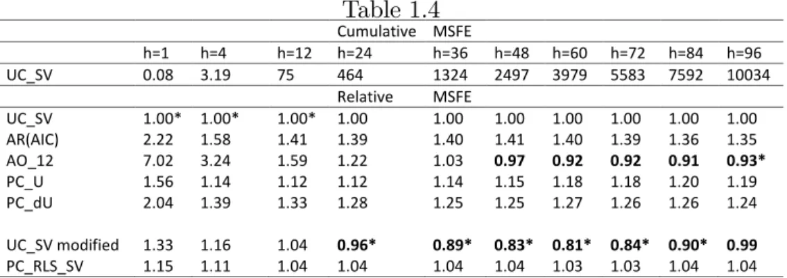
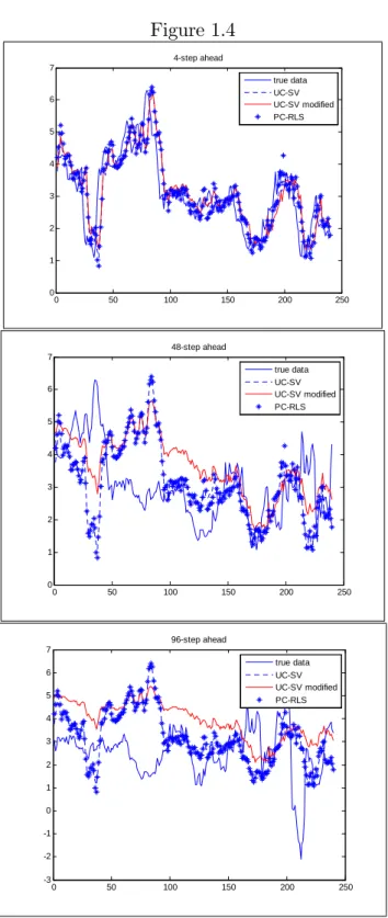
The results are presented in Table 4 for the forecasting period 1984 to the end of the sample and forecast horizonsh= 1;4;12;24;36;48;60;72;84;96months. The UC-SV model is used as the benchmark. Consistent with the results of Stock and Watson (2007), the UC_SV performs best at short horizons up to 12 months with the two models with random
level shifts close second and third. At longer forecasting horizons, the UC_SV model with random level shifts performs best with reductions in MSFE of up to 20% at the 5 years horizon. At the longest horizon considered, 96 months, the naive AO forecasts are the best but the methods is, however, very unreliable at short horizons. The forecasts of the basic UC_SV model, the UC_SV model with random level shifts and the Phillips Curve model with random level shifts are presented in Figure 4 for foreacst horizons h = 4; 48 and 96
months ahead. The results show how the the UC_SV model with random level shifts tracks actual in‡ation more closely.
Overall, the UC_SV model with random level shifts provides substantial improvements over the standard UC_SV model at long horizons and is still competitive at short horizons.
1.6.3 Exchange rates
Since the work by Meese and Rogo¤ (1983a,b), the prevalent view has been that a simple random walk model has a better forecasting performance than macroeconomic models of exchange rates. However, the forecasting failure of fundamental models may not be due to the lack of correlation between fundamentals and exchange rate ‡uctuations but may be the outcome of instabilities in the relationships. Such instabilities have been documented by Rossi (2006) and Kilian and Taylor (2003), among others. Using tests robust to parameter instability, they reached the conclusion that exchange rates are not random walks in-sample. Here, we shall directly consider two popular fundamentals-based models of exchange rate allowing for time variations in the parameters and compare their forecasting performance to the simple random walk model.
The …rst is the Uncovered Interest Rate Parity Model (UIRP) which speci…es that the …rst-di¤erences of the logarithm of the bilateral nominal exchange rate, st, is determined by
st+1 st= 1+ 2zt+ t+1
where zt = ft st, with ft the long-run equilibrium level of the nominal exchange rate determined by macroeconomic fundamentals. In the UIRP model,ft= (it it) +st, where
it it is the short-term interest rate di¤erence between the home and foreign countries. The UIRP model with time-varying parameters, can then be written as:
st+1 st= 1t+ 2t(it it) + t+1 (1.11)
We shall apply this model using monthly data (not seasonally adjusted) of the exchange rates for the Japanese Yen and the Canadian Dollar relative to the US dollar. The exchange rate data were obtained from the Board of Governors of the Federal Reserve System. The monthly interest rates for government securities and bonds for Japan, Canada and the USA were obtained from the IMF’s International Financial Statistics database. The sample is from 1971:1 to 2012:4. Data prior to 1984 are used for the in-sample estimation, and we consider forecasts up to 24-months ahead.
The second model is one with the so-called Taylor Rule fundamentals as proposed by Molodtsova and Papell (2007). In this model, the interest rate of the home country is assumed to follow a Taylor rule (Taylor, 1993) given by:
it= t+ ( t T) + ytgap+r
where t is the in‡ation rate, T is the target level of in‡ation,ytgap is the output gap and r is the equilibrium level of the real interest rate. If we assume that the coe¢ cients of the Taylor rule in the foreign countries are similar to the those of the home country, we obtain, in …rst-di¤erences, that: it it = (1 + )( t t) + (y gap t y gap t )
Then the exchange rate model with time varying parameters is:
st+1 st= 1t+ 2t( t t) + 3t(y gap
t y
gap
t ) + t+1 (1.12)
For the in‡ation series, we use monthly data of the CPI for all items from the Federal banks of St. Louis database and calculate the compounded annual rate of change. The output
gap series are constructed based on industrial production indices (seasonally adjusted) as the percentage di¤erence between actual and potential output at time t, where potential output is measured by the linear time trend in output.
The models with time variations in the parameters that we consider are; 1) UIRP_level shift: Model (1.11) withK2t= 0; 2) UIRP_RLS: Model (1.11) withK1t= 0; 3) UIRP_Kt: Model (1.11) withK1t=K2tso that both parameters are allowed to change according to the same latent Bernoulli variable; 4) UIRP_ K1t; K2t: Model (1.11) with K1t 6= K2t so that both parameters are allowed to change according to di¤erent latent Bernoulli variables; 5) Taylor-Rule_level shift: Model (1.12) withK2t=K3t= 0; 6) Taylor-Rule_RLS (in‡ation): Model (1.12) with K1t = K3t = 0; 7) Taylor-rule_RLS (output gap): Model (1.12) with
K1t=K2t= 0; 8) Taylor-Rule_constant+in‡ation_Kt: Model (1.12) with K1t=K2t and K3t= 0; 9) Taylor-Rule_constant+output_Kt: Model (1.12) withK1t=K3tandK2t= 0; 10) Taylor-Rule_constant+in‡ation_K1t; K2t: Model (1.12) withK1t 6=K2t and K3t= 0; 11) Taylor-Rule_constant+output_K1t; K2t: Model (1.12) with K1t 6= K3t and K2t = 0. We also consider a random walk model with random level shifts. In all cases, mean-reversion in the parameters is allowed and, in all cases with a single latent Bernoulli random variable, the covariatewtused to model the time-varying probabilities is the change in stock returns, constructed from the logarithm of the monthly S&P stock price index. For models with two Bernoulli random variables, the additional covariate is the change in M2. The popular competing models to which we make comparisons are: 1) the random walk model; 2) the UIRP with constant coe¢ cients; 3) the Taylor-Rule with constant coe¢ cients.
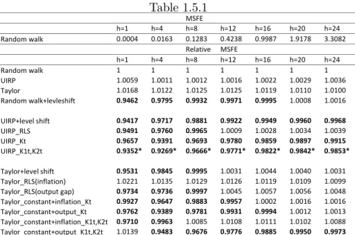
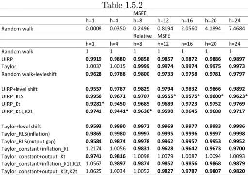
The forecasting period is 1969:1 to the end of the sample and we consider the forecast horizonsh= 1;4;8;12;16;20;24 months. The results are presented in Table 5.1 for Canada and 5.2 for Japan. For Canada, the best forecasting models are the various versions of the UIRP with random level shift parameters and the random walk model with random level shifts. The model with the smallest MSFE for all horizons is the UIRP_K1t; K2tfor which both parameters are allowed to change according to di¤erent latent Bernoulli variables. The gains in forecast accuracy range from 2% to 8%. These reductions are more modest
in comparisons with the other series analyzed but still important given the di¢ culty in forecasting exchange rates. The results are broadly similar for Japan, though in this case the UIRP_RLS version has smallest MSFE at longer horizons.
1.6.4 Interest rate forecasting
Another variable of interest, which has attracted attention from a forecasting perspective is the U.S. T-bill rates. Various studies have shown that it exhibits structural instability in both mean and variance, see, e.g. Garcia and Perron (1996), Gray (1996), Ang and Bekaert
(2002) and Pesaran and Timmermann (2006). We use monthly data on the 3-months
Treasury Bill rates from 1947:07-2002:12, obtained from the Federal Bank of St. Louis database. The period prior to 1968:12 is used for in-sample estimation, and we consider forecasting horizons of 12, 24, 36, 48 and 60 months. The basic model adopted is a simple AR(1) process with stochastic volatility given by:
yt = 1t+ 2tyt 1+ ";t"t ln 2";t = ln 2";t 1+v";t
In all cases, we allow mean-reversion in the parameters and the covariatewtused to model the time-varying probabilities of shifts is the growth rate of GDP when a single latent Bernoulli varaible is present. When two are present, the additional covariate is the absolute change in stock returns (S&P 500). We consider …ve possible speci…cations: 1) AR_level shift_SV (K2t = 0 and Kt 6= 0); 2) AR_RLS_SV (K1t = 0 and Kt 6= 0); 3) AR_RLS (K1t= 0andKt = 0); 4) AR_level shift (K2t= 0andKt = 0); 5) AR_K1t_K2twithK1t
and K2t allowed to be di¤erent latent Bernoulli processes. The performance of the models is assessed relative to four commonly used forecasting methods: 1) a 5 years rolling average (used as the benchmark model); 2) a 10 years rolling average; 3) a recursive OLS based an a …rst-order autoregression with …xed parameters; 4) a time-varying probability model in which 2t is modelled as a random walk.
h = 12;24;36;48;60 months. Consider …rst the results for the longest forecasting period 1968-2002. Here, the best forecasting model for all horizons is the AR_RLS with the coe¢ cient on the lagged dependent variable allowed to follow a random level shift process. The gains in forecast accuracy vary between 6 and 17% and increase as the forecasting horizon increases. The same model with added stochastic volatility is the second best. We then separate the forecasting period into three decades: the 70s, the 80s and the 90. In the 70s, the 5 years rolling average is overall the best, though all models perform about the same with the exception of the TVP and the AR_K1t_K2t models whose performances are inferior. For the 80s, the best forecasting models are again the AR_RLS with the coe¢ cient on the lagged dependent variable allowed to follow a random level shift process and its variant that incorporate a stochastic volatility component. The improvements in forecast accuracy are quite impressive, ranging from 14% at short-horizon to 60% at long-horizon relative to the benchmark model. For the 90s, the best performing model is the AR_K1t_K2tfor which both the mean and autoregressive coe¢ cient are changing according to di¤erent latent Bernoulli processes. Note, however, that all models with random level shifts in parameters perform better than the benchmark 5 years rolling average.
Overall, the evidence again indicates that important gains in forecast accuracy can be obtained using our forecasting models and that they are robust in the sense that in no case do hey performs substantially worse than the popular forecasting methods. Overall, for the application, the AR_RLS model with the coe¢ cient on the lagged dependent variable allowed to follow a random level shift process is the best and most robust across the various speci…cations considered.
1.7 Conclusion
We proposed a forecasting framework based on modeling the parameters as random level shift processes dictated by a Bernoulli process for the occurrence of shifts and a normal random variable for its magnitude. Some or all of the parameters of the model can be allowed to change and the latent variables that dictate the changes can be common or
di¤erent for each parameters. Also, the variance of the errors may change in a similar manner. To improve the forecasting performance we augmented the basic model to allow the probability of shifts to be a function of some covariates which can be forecasted and to incorporate a mean-reversion mechanism such that the parameters tend to revert back to the pre-forecast average.
Our model can be cast into a non-linear non-Gaussian state space framework for which standard Kalman …lter type algorithms cannot be used. To provide a computationally e¢ cient method of estimation, we rely on recent developments on particle …ltering methods. Simulations show that the estimation method provides very reliable results in …nite samples. The parameters are estimated precisely and the …ltered estimates of the time path of the parameters follow closely the true process.
We apply our forecasting model to a variety of series which have been the object of considerable attention from a forecasting point of view. These include the equity premium, in‡ation, exchange rates and the Treasury bill interest rates. In each case, we compare the forecast accuracy of our model relative to the most important forecasting methods used applicable for each di¤erent variable. We also consider di¤erent forecasting sub-samples or periods. The results show clear gains in forecasting accuracy, sometimes by a very wide margin; e.g., over 80% reduction in mean squared forecast error for the equity premium over all popular contenders.
Finally, note that given the availability of the proper code for estimation and forecasting, the method is very ‡exible and easy to implement. For a given forecasting model, all that is required by the users are: 1) which parameters (including the variance of the errors if desired) are subject to change; 2) whether the same or di¤erent latent Bernoulli processes dictates the timing of the changes in each parameters; 3) which covariates are potential explanatory variable to model the probability of shifts.