www.ssoar.info
A comparison of mean-variance efficiency tests
Amengual, Dante; Sentana, Enrique Postprint / Postprint
Zeitschriftenartikel / journal article
Zur Verfügung gestellt in Kooperation mit / provided in cooperation with: www.peerproject.eu
Empfohlene Zitierung / Suggested Citation:
Amengual, D., & Sentana, E. (2009). A comparison of mean-variance efficiency tests. Journal of Econometrics, 154(1), 16-34. https://doi.org/10.1016/j.jeconom.2009.06.006
Nutzungsbedingungen:
Dieser Text wird unter dem "PEER Licence Agreement zur Verfügung" gestellt. Nähere Auskünfte zum PEER-Projekt finden Sie hier: http://www.peerproject.eu Gewährt wird ein nicht exklusives, nicht übertragbares, persönliches und beschränktes Recht auf Nutzung dieses Dokuments. Dieses Dokument ist ausschließlich für den persönlichen, nicht-kommerziellen Gebrauch bestimmt. Auf sämtlichen Kopien dieses Dokuments müssen alle Urheberrechtshinweise und sonstigen Hinweise auf gesetzlichen Schutz beibehalten werden. Sie dürfen dieses Dokument nicht in irgendeiner Weise abändern, noch dürfen Sie dieses Dokument für öffentliche oder kommerzielle Zwecke vervielfältigen, öffentlich ausstellen, aufführen, vertreiben oder anderweitig nutzen.
Mit der Verwendung dieses Dokuments erkennen Sie die Nutzungsbedingungen an.
Terms of use:
This document is made available under the "PEER Licence Agreement ". For more Information regarding the PEER-project see: http://www.peerproject.eu This document is solely intended for your personal, non-commercial use.All of the copies of this documents must retain all copyright information and other information regarding legal protection. You are not allowed to alter this document in any way, to copy it for public or commercial purposes, to exhibit the document in public, to perform, distribute or otherwise use the document in public.
By using this particular document, you accept the above-stated conditions of use.
Accepted Manuscript
A comparison of mean-variance efficiency tests
Dante Amengual, Enrique Sentana
PII: S0304-4076(09)00147-X DOI: 10.1016/j.jeconom.2009.06.006
Reference: ECONOM 3213
To appear in: Journal of Econometrics
Received date: 2 May 2008 Revised date: 3 June 2009 Accepted date: 22 June 2009
Please cite this article as: Amengual, D., Sentana, E., A comparison of mean-variance efficiency tests.Journal of Econometrics(2009), doi:10.1016/j.jeconom.2009.06.006
This is a PDF file of an unedited manuscript that has been accepted for publication. As a service to our customers we are providing this early version of the manuscript. The manuscript will undergo copyediting, typesetting, and review of the resulting proof before it is published in its final form. Please note that during the production process errors may be discovered which could affect the content, and all legal disclaimers that apply to the journal pertain.
A
CCEPTED
MANUSCRIPT
ACCEPTED MANUSCRIPT
A comparison of mean-variance efficiency tests
∗
Dante Amengual
Department of Economics, Princeton University,
Fisher Hall, Princeton, NJ 08544-1021, USA
[email protected]
Enrique Sentana
CEMFI, Casado del Alisal 5, E-28014 Madrid, Spain
[email protected]
Revised: May 2009
Abstract
We analyse the asymptotic properties of mean-variance efficiency tests based on gen-eralised methods of moments, and parametric and semiparametric likelihood procedures that assume elliptical innovations. We study the trade-off between efficiency and robust-ness, and prove that the parametric estimators provide asymptotically valid inferences when the conditional distribution of the innovations is elliptical but possibly misspecificed and heteroskedastic. We compare the small sample performance of the alternative tests in a Monte Carlo study, and find some discrepancies with their asymptotic properties. Finally, we present an empirical application to US stock returns, which rejects the mean-variance efficiency of the market portfolio.
Keywords: Adaptivity, Elliptical Distributions, Financial Returns, Portfolio choice, Semiparametric Estimators.
JEL: C12, C13, C14, C16, G11, G12
∗We would like to thank Manuel Arellano, Christian Bontemps, Marcelo Fernandes, Gabriele Fiorentini, Javier
Mencía, Nour Meddahi, Francisco Peñaranda and Kevin Sheppard, as well as audiences at Queen Mary, the Imperial College Financial Econometrics Conference (London, 2007), the XV Finance Forum (Majorca), and the XXXII Symposium on Economic Analysis (Granada) for useful comments and discussions. The suggestions of an associate editor and two anonymous referees have also greatly improved the exposition. Of course, the usual caveat applies. Financial support from the Spanish Ministry of Science and Innovation through grant ECO 2008-00280 (Sentana) is gratefully acknowledged.
A
CCEPTED
MANUSCRIPT
ACCEPTED MANUSCRIPT
1
Introduction
Mean-variance analysis is widely regarded as the cornerstone of modern investment theory. Despite its simplicity, and the fact that more than five and a half decades have elapsed since Markowitz published his seminal work on the theory of portfolio allocation under uncertainty (Markowitz (1952)), it remains the most widely used asset allocation method. A portfolio with excess returns is mean-variance efficient with respect to a given set of assets with excess
returns r if it is not possible to form another portfolio of those assets and with the same
expected return as but a lower variance, or more appropriately, with the same variance but
a higher expected return. Despite the simplicity of this definition, testing for mean-variance efficiency is of paramount importance in many practical situations, such as mutual fund perfor-mance evaluation (see De Roon and Nijman (2001) for a recent survey), gains from portfolio diversification (Errunza, Hogan and Hung (1999)), or tests of linear factor asset pricing models, including the capital asset pricing model and arbitrage pricing theory, as well as other empirically oriented asset pricing models (see e.g. Campbell, Lo and MacKinlay (1997) or Cochrane (2001) for textbook treatments).
As is well known, will be mean-variance efficient with respect to r in the presence of a
riskless asset if and only if the intercepts in the theoretical least squares projection of r on a
constant and are all 0 (see Jobson and Korkie (1982), Gibbons, Ross and Shanken (1989)
and Huberman and Kandel (1987)). Therefore, it is not surprising that this early literature resorted to ordinary least squares (OLS) to test those theoretical restrictions empirically. If the distribution of r conditional on (and their past) were multivariate normal, with a linear
meana+b and a constant covariance matrixΩ, then OLS would produce efficient estimators
of the regression intercepts a, and consequently, optimal tests of the mean-variance efficiency restrictions0 :a=0. In addition, it is possible to derive an version of the test statistic whose
sampling distribution in finite samples is known under exactly the same restrictive distributional assumptions (see Gibbons, Ross and Shanken (1989)). In this sense, this -test generalises the
-test proposed by Black, Jensen and Scholes (1972) in univariate contexts.
However, many empirical studies withfinancial time series data indicate that the distribution of asset returns is usually rather leptokurtic. For that reason, MacKinlay and Richardson (1991) proposed alternative tests based on the generalised method of moments (GMM) that are robust to non-normality, unlike traditional OLS test statistics.
semipara-A
CCEPTED
MANUSCRIPT
ACCEPTED MANUSCRIPT
metric estimation and testing methodology that enabled them to obtain optimal mean-variance efficiency tests under the assumption that the distribution of r conditional on (and their
past) is elliptically symmetric. Specifically, HLV showed that their proposed estimators ofaandb are adaptive under the aforementioned assumptions of linear conditional mean and constant con-ditional variance, which means that they are as efficient asinfeasible maximum likelihood (ML) estimators that use the correct parametric elliptical density with full knowledge of its shape pa-rameters. Elliptical distributions are attractive in this context because they relate mean-variance analysis with expected utility maximisation (see e.g. Chamberlain (1983), Owen and Rabinovitch (1983) and Berk (1997)). Moreover, they generalise the multivariate normal distribution, but at the same time they retain its analytical tractability irrespective of the number of assets.
Nevertheless, thefinite sample performance of such semiparametric inference procedures may not be well approximated by the first-order asymptotic theory that justifies them. For that reason, an alternative approach worth considering is an unrestricted ML estimator based on the correct elliptical distribution, but which includes the unknown shape parameters as additional arguments in the maximisation algorithm (see e.g. Kan and Zhou (2006)). However, unless we are careful, this last approach may provide misleading inferences if the relevant conditional distribution does not coincide with the assumed one, even if both are elliptical. The same applies to elliptically-based restricted maximum likelihood estimators that keep the shape parameters
fixed to some a priori values, even if the assumed conditional distribution is correct, unless the chosen values either imply multivariate normality, in which case such restricted estimators will reduce to the OLS-GMM ones, or they happened to coincide with the true values, in which case those restricted estimators would be identical to the infeasible ML estimators. Similarly, the HLV approach may also lead to erroneous inferences if the true conditional distribution is either heteroskedastic or asymmetric.
Although atfirst sight these considerations may only seem interesting for theoretically inclined econometricians, they are also relevant for applied researchers because in practice the substantive conclusions about the mean-variance efficiency of a candidate portfolio can be rather sensitive to the distributional assumptions made, as our empirical results confirm.
In this context, the purpose of our paper is to shed some light on such efficiency-consistency trade-offs in the context of mean-variance efficiency tests. To do so, we will first exploit the results in Fiorentini and Sentana (2007) to derive the asymptotic properties of the estimators of the regression intercepts,a, and slopes,b, based on GMM, HLV and elliptically-based parametric ML procedures under correct specification. Then, we will extend our results to characterise
A
CCEPTED
MANUSCRIPT
ACCEPTED MANUSCRIPT
how those asymptotic properties change under some specific forms of misspecification that are potentially relevant in practice in view of some observed characteristics of asset returns, which we will take into consideration in our empirical application. In particular, we study those situations in which the distribution of the innovations is:
(i) elliptical but different from the parametric one assumed for estimation purposes, which will often be chosen for convenience or familiarity,
(ii) elliptical but conditionally heteroskedastic, which arises when the distribution of excess returns for the assets r and the reference portfolio, , is elliptical, and
(iii) not elliptically symmetric.
In addition, given that it is far from trivial to obtain exact finite sample distributions once we abandon the Gaussianity assumption, we also analyse the reliability of the usual asymptotic approximations by Monte Carlo methods.1
Our main asymptotic results are:
1. Under correct specification, not only the HLV procedure but also the unrestricted para-metric estimators are adaptive, in the sense that they are as efficient as if one had full knowledge of the true conditional distribution, including its shape parameters.
2. Pseudo-ML (PML) estimators of the regression intercepts and slopes based on the Student
remain consistent when the conditional distribution is elliptical but not irrespective of whether the degrees of freedom are estimated or fixed a priori. In addition, the restricted esti-mator will still be consistent when the true conditional distribution is but with a number of degrees of freedom different from the one assumed a priori. Both these PML estimators are also consistent when the conditional distribution is elliptical but conditionally heteroskedastic. In all these cases, we provide correct expressions for the asymptotic covariance matrices of the regres-sion coefficients, and explain how applied researchers can robustify their inferences in practice. The HLV procedure also seems to yield consistent estimators in a conditionally heteroskedastic elliptical context, which confirms related results by Hodgson (2000) in a univariate framework.
3. The -based PML estimators seem to be systematically more efficient than the GMM estimators when the conditional distribution of r given is elliptical, irrespective of whether
or not it is or conditionally homoskedastic. In addition, estimating the degrees of freedom parameter instead of fixing its value a priori typically leads to efficiency gains.
4. Only the GMM estimator of the regression intercepts provides reliable inferences in the
1See Beaulieu, Dufour and Khalaf (2007b) for a method to obtain the exact distribution of the Gibbons, Ross
A
CCEPTED
MANUSCRIPT
ACCEPTED MANUSCRIPT
presence of asymmetries.
Although our Monte Carlo results are broadly in line with these theoretical conclusions, they also point out two interesting facts. First, we find that the HLV tests typically have much larger size distortions in finite samples than the other tests. Secondly, they have smaller size-adjusted power than the -based PML tests, although the differences are very small when the latter are asymptotically suboptimal.
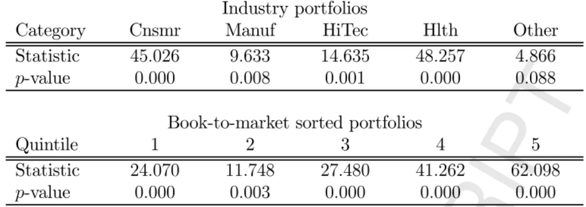
Finally, we apply those different procedures to test the mean-variance efficiency of the US aggregate stock market portfolio with respect to industry portfolios, and the book-to-market sorted portfolios popularised by Fama and French (1993). We do so using monthly data over the period July 1962 to June 2007. The results that we obtain for industry portfolios indicate that the Student -based test clearly rejects the efficiency of the market portfolio, while the GMM test is borderline, and the HLV based test fails to reject. Given our Monte Carlo results, this contradicting behaviour is partly due to the lack of reliability of the nonparametric estimates of the asymptotic covariance matrix implicit in the HLV procedure, even though we use the improved procedure recommended by Fiorentini and Sentana (2007). In contrast, all three tests reject the mean-variance efficiency of the market portfolio relative to the book-to-market sorted portfolios of Fama and French (1993).
Importantly, we also assess the adequacy of our parametric assumptions by computing spec-ification tests against heteroskedasticity, asymmetries, and departures from the distribution in higher order moments. We find that while the assumption of Gaussianity is overwhelmingly re-jected in both data sets, the evidence against a multivariate distribution is weak. Nevertheless, wefind quite strong evidence against conditional homoskedasticity, which confirms the usefulness of our robust asymptotic covariance expressions. In view of the trade-offs between efficiency and consistency that we characterise in our theoretical analysis, these empirical results suggest that it is probably worth using the multivariate distribution for the purposes of testing mean-variance efficiency, as long as empirical researchers bear in mind that such a distributional assumption may be wrong, and robustify their inferences accordingly.
The rest of the paper is organised as follows. In section 2, we introduce the model and the three aforementioned estimation procedures, obtain their asymptotic distributions under the assumption that the innovations are elliptical, and discuss the testing implications of those results. Then in section 3 we derive the asymptotic properties of those estimators in alternative misspecified contexts. An extensive Monte Carlo evaluation of the different parameter estimators and testing procedures can be found in section 4, while section 5 reports our empirical results.
A
CCEPTED
MANUSCRIPT
ACCEPTED MANUSCRIPT
Finally, we present our conclusions and suggestions for future work in section 6. Proofs and auxiliary resutls are gathered in the appendices.
2
Econometric methods
2.1
Model description
Consider the following multivariate, conditionally homoskedastic, linear regression model r=a+b +u=a+b +Ω12ε∗ (1)
whereΩ12 is an× “square root” matrix such thatΩ12Ω12 =Ω,ε∗ is a standardised vector
martingale difference sequence satisfying(ε∗| −1;γ0ω0) =0and(ε∗| −1;γ0ω0) =
I, γ0 = (a0b0), ω = (Ω), the subscript 0 refers to the true values of the parameters,
and −1 denotes the information set available at − 1, which contains at least past values
of and r. To complete the conditional model, we need to specify the distribution of ε∗.
We shall initially assume that conditional on and −1, ε∗ is independent and identically
distributed as some particular member of the elliptical family with a well defined density, or
ε∗
| −1;γ0ω0η0 ∼ (0Iη0) for short, where η are some additional parameters
that determine the shape of the distribution of =ε∗0ε∗.2 The most prominent example is the
spherical normal distribution, which we denote by η=0. Another popular and more empirically realistic example is a standardised multivariate with 0 degrees of freedom, or (0I 0)
for short. As is well known, the multivariate Student approaches the multivariate normal as
0 → ∞, but has generally fatter tails. For that reason, we define as 1, which will always
remain in thefinite range [0,1/2) under our assumptions. Following Zhou (1993), we also consider two other illustrative examples: a Kotz distribution and a discrete scale mixture of normals.
The original Kotz distribution (see Kotz (1975)) is such that is a gamma random variable
with mean and variance [(+ 2)0+ 2], where
=(2|η)[( + 2)]−1
is the coefficient of multivariate excess kurtosis ofε∗ (see Mardia (1970)). The Kotz distribution
nests the multivariate normal distribution for= 0, but it can also be either platykurtic ( 0) or leptokurtic ( 0). Although such a nesting provides an analytically convenient generalisation
2Ifε∗
is distributed as a spherically symmetric multivariate random vector, then we can writeε∗ =u, where uis uniformly distributed on the unit sphere surface inR, and =
p
ε∗0
ε∗ is a nonnegative random variable that is independent of u. Assuming that
£ 2
¤
∞, then ε∗
can be standardised by setting
£ 2 ¤ =, so that [ε∗ ] =0and[ε∗] =I.
A
CCEPTED
MANUSCRIPT
ACCEPTED MANUSCRIPT
of the multivariate normal, the density of a leptokurtic Kotz distribution has a pole at 0, which is a potential drawback from an empirical point of view.
For that reason, we also consider a standardised version of a two-component scale mixture of multivariate normals,3 which can be generated as
ε∗ = + (1−)√κ p + (1−)κ ·ε ◦ (2) where ε◦
is a spherical multivariate normal, is an independent Bernoulli variate with( = 1) = and κ is the variance ratio of the two components. Not surprisingly, will be a
two-component scale mixture of 20. As all scale mixtures of normals, the distribution of ε∗ is
leptokurtic, so that
= (1−)(1−κ) 2 [+ (1−)κ]2 ≥0
with equality if and only if either κ = 1, = 1 or = 0, when it reduces to the spherical normal.4 In this sense, a noteworthy property of all discrete mixtures of normals is that their density and moments are always bounded.
Figure 1 plots the densities of a normal, a Student , a platykurtic Kotz distribution and a discrete scale mixture of normals in the bivariate case. Although they all have concentric circular contours because we have standardised and orthogonalised the two components, their densities can differ substantially in shape, and in particular, in the relative importance of the centre and the tails. They also differ in the degree of cross-sectional “tail dependence” between the components, the normal being the only example in which lack of correlation is equivalent to stochastic independence. Allowing for dependence beyond correlation is particularly important in the context of multiple financial assets, in which the probability of the joint occurrence of several extreme events is regularly underestimated by the multivariate normal distribution.
2.2
Parameter estimation
The purpose of this section is to derive the asymptotic variances of the three estimators of the regression intercepts, a, and slopes, b, mentioned in the introduction (namely, OLS-GMM, as well as elliptically symmetric parametric and semiparametric procedures) under the assumption that the conditional distribution of the innovations ε∗ is indeed spherical.
3The extension of our analytical results to discrete scale mixtures of normals with multiple components would
be fairly straightforward. As is well known, multiple component mixtures can arbitrarily approximate the more empirically realistic continuous mixtures of normals such as symmetric versions of the hyperbolic, normal inverse Gaussian, normal gamma mixtures, Laplace, etc.
4In general, though, we require at least sixth moments to globally identifyη= (
κ)0. Since the labels of the components are arbitrary, we also need to impose either 0≤κ≤1or≥12
A
CCEPTED
MANUSCRIPT
ACCEPTED MANUSCRIPT
2.2.1 Maximum likelihood estimators
Letφ= (γ0ω0η)0 ≡(θ0η)0 denote the2+(+ 1)2 + parameters of interest, which we assume variation free. The log-likelihood function of a sample of size based on a particular parametric spherical assumption will take the form (φ) = P=1(φ), with (φ) = (θ) +
(η) +[(θ)η], where (θ) = −12ln|Ω| corresponds to the Jacobian, (η) to the constant
of integration of the assumed density, and [(θ)η] to its kernel, where (θ) =ε∗0(θ)ε∗(θ), ε∗
(θ) =Ω− 12
ε(θ) andε(θ) =y−a−b .5
Let s(φ) denote the score function (φ)φ, and partition it into three blocks, s(φ),
s(φ), and s(φ), whose dimensions conform to those ofγ, ω andη, respectively. A
straight-forward application of expression (2) in Fiorentini and Sentana (2007) implies that s(φ) = µ 1 ¶ ⊗[(θ)η]Ω−1ε(θ) (3) s(φ) = 1 2D 0 £ Ω−1⊗Ω−1¤{[(θ)η]ε(θ)ε0(θ)−Ω} (4)
where D is the duplication matrix of order such that (Ω) = D(Ω) (see Magnus
and Neudecker (1988)), while the scalar
[(θ)η] =−2[(θ)η]
reduces to
( + 1)[1−2+(θ)]
in the Student case, to
[( + 2)−1(θ) + 2][( + 2)+ 2]
in the case of the Kotz distribution, to
[+ (1−)κ]· + (1−)κ−(2+1)exph −[+(1−2)κκ](1−κ)(θ) i + (1−)κ−2exph−[+(1−)κ](1−κ) 2κ (θ) i (5)
for the two-component mixture, and to 1under Gaussianity.6
Given correct specification, the results in Crowder (1976) imply that the score vector s(φ)
evaluated at the true parameter values has the martingale difference property. His results also imply that, under suitable regularity conditions, which typically require that both and 2
5Fiorentini, Sentana and Calzolari (2003) provide expressions for () and
[(θ) ] in the multivariate Student case, which under normality collapse to−(2) logand−1
2(θ), respectively.
6See Fiorentini, Sentana and Calzolari (2003) for numerically reliable expressions for
(φ)and(φ)in the multivariate case.
A
CCEPTED
MANUSCRIPT
ACCEPTED MANUSCRIPT
are strictly stationary processes with absolutely summable autocovariances, the asymptotic dis-tribution of the unrestricted ML estimator will be given by the following expression
√ ³ ˆ φ−φ0 ´ −→£0I−1(φ0) ¤ where I(φ0) =[I(φ0)|φ0], I(φ) = [s(φ)| −1;φ] =−[h(φ)| −1;φ]
and h(φ) denotes the Hessian function s(φ)φ0 =2(φ)φφ0. These expressions adopt
particularly simple forms for our model of interest:
Proposition 1 If ε∗
| −1;φ in (1) is (0Iη) with density exp[(η) +(η)], then the only non-zero elements of I(φ0) will be:
I(φ) = m(η) µ 1 2 ¶ ⊗Ω −1 I(φ) = m(η) 2 D 0 £ Ω−1⊗Ω−1¤D + m(η)−1 4 D 0 £ (Ω−1)0(Ω−1)¤D I(φ) = 1 2m(η)D 0 (Ω− 1) I(φ) = [s(φ)|φ] =−[h(φ)|φ] where m(η) = ½ 2[(θ)η] (θ) ¯ ¯ ¯ ¯φ ¾ = ½ 2[(θ)η] (θ) +[(θ)η] ¯ ¯ ¯ ¯φ ¾ m(η) = + 2 h 1 + n[(θ)η] ¯ ¯ ¯φoi= ½ 2[(θ)η] 2 (θ) ( + 2) ¯ ¯ ¯ ¯φ ¾ + 1 m(η) = ∙½ [(θ)η] (θ) −1 ¾ e0(φ) ¯ ¯ ¯ ¯φ ¸ =− ½ (θ) [(θ)η] η0 ¯ ¯ ¯ ¯φ ¾
In the multivariate standardised Student case, in particular: m() = ( +) (−2) ( ++ 2) m() = ( +) ( ++ 2) m() = − 2 ( + 2)2 (−2) ( +) ( ++ 2)
which under normality reduce to 1, 1 and0, respectively (see Fiorentini, Sentana and Calzolari (2003)). As for the Kotz distribution, we can combine the moments of the gamma and reciprocal gamma random variables to show that
m() = 1 [( + 2)+ 2]2 ½ ( + 2)22 −[( + 2)+ 2] + 4[( + 2)+ 1] ¾ (6)
A
CCEPTED
MANUSCRIPT
ACCEPTED MANUSCRIPT
as long as ( −2)( + 2) when 6= 0, m() = 1 [( + 2)+ 2]2 ½ ( + 2)22+ 4 [ + ( + 2)+ 2] + 4(+ 2) ¾ andm() = 0 ∀, as in the Gaussian case. Finally, we provide the relevant expressions for the
case of the two-component scale mixture of normals in Supplemental Appendix D. The next result follows directly from Proposition 1:
Proposition 2 If ε∗| −1;φ0 in (1) is (0Iη0) with density exp[(η) + (η)] such that m(η0)∞, and both and 2 are strictly stationary processes with absolutely summable autocovariances, then
√ (γˆ −γ0)→ £ 0I−1(φ0) ¤ where I−1(φ) = 1 m(η) µ (1 +2 2) −2 −2 12 ¶ ⊗Ω (7)
= ( |φ) and 2 = ( |φ), so that can be interpreted as the Sharpe ratio of the reference portfolio.
Importantly, expression (7) is valid regardless of whether or not the shape parametersη are
fixed to their true valuesη0, as in the infeasible ML estimator,ˆa say, or jointly estimated with θ, as in the unrestricted one,ˆa say. The reason is that the scores corresponding to the mean
parameters,s(φ0), and the scores corresponding to variance and shape parameters,s(φ0)and
(φ0), respectively, are asymptotically uncorrelated under our sphericity assumption in view of
Proposition 1.
2.2.2 GMM estimators
MacKinlay and Richardson (1991) developed a robust test of mean-variance efficiency by using Hansen’s (1982) GMM methodology. If we callR0≡( r0), the orthogonality conditions
that they considered are
[m(R;γ)] =0 m(R;γ) = µ 1 ¶ ⊗ε(γ) (8)
The advantage of working within a GMM framework is that under fairly weak regularity conditions inference can be made robust to departures from the assumption of normality, condi-tional homoskedasticity, serial independence or identity of distribution. But since the above mo-ment conditions exactly identifyγ, the unrestricted GMM estimators coincide with the Gaussian
A
CCEPTED
MANUSCRIPT
ACCEPTED MANUSCRIPT
pseudo ML estimators, which in turn coincide with the equation by equation OLS estimators in the regression of each element of r on a constant and . An alternative way of reaching
the same conclusion is by noticing that the influence function m(R;γ) is a full-rank linear
transformation with time-invariant weights of the Gaussian pseudo-score s(θη =0).7
It is convenient to derive an expression for the asymptotic covariance matrix ofγˆ under
innovations:
Proposition 3 If ε∗
| −1;φ in (1) is (0I) with density function (ε∗;%), where % are some shape parameters, and both and2 are strictly stationary processes with absolutely summable autocovariances, then
√ (ˆγ −γ0)→[0C(φ0)] (9) where C(φ) =A−1(φ)B(φ)A−1(φ) A(φ) =−[h(θ0)|φ] =[A(φ)|φ] A(φ) =−[h(θ;0)| −1;φ] = µ 1 2 ¶ ⊗Ω−1 B(φ) = [s(θ0)|φ] =[B(φ)|φ] B(φ) =[s(θ;0)| −1;φ] =A(φ) so that C(φ0) = µ (1 +2 020) −020 −020 120 ¶ ⊗Ω0 (10)
Importantly, note thatC(φ0)does not depend on the specific distribution for the innovations
that we are considering, regardless of whether or not the conditional distribution ofε∗
is spherical,
as long as it is 8
2.2.3 HLV elliptically symmetric semiparametric estimators
HLV proposed a semiparametric estimator of multivariate linear regression models that up-dates ˆθ (or any other root- consistent estimator) by means of a single scoring iteration
7The obvious GMM estimator of ω is given byΩˆ = 1
P
=1ε(γˆ )ε0(ˆγ ), which is the sample analogue to the residual covariance matrix.
8The asumption of constant conditional third and fourth moments implicit in the assumption of
innova-tions also implies that the optimal GMM estimators of Meddahi and Renault (1998) do not offer any asymptotic efficiency gains overˆa .
A
CCEPTED
MANUSCRIPT
ACCEPTED MANUSCRIPT
without line searches. The crucial ingredient of their method is the so-called elliptically symmet-ric semiparametsymmet-ric efficient score (see e.g. Proposition 7 in Fiorentini and Sentana (2007)):
˚s(φ0) =s(φ0)−W(φ0) ½∙ [(θ0)η0] (θ0) −1 ¸ −(+ 2)2 0+ 2 ∙ (θ0) −1 ¸¾ where W0(φ) =£ 0 0 1 20(Ω− 1)D ¤
in the case of model (1). In fact, the special structure of W(φ) implies that we can update the
GMM estimator of γ by means of the following simple Berndt, Hall, Hall and Hausman (1974) (BHHH) correction: " X =1 s(φ0)s0(φ0) #−1 X =1 s(φ0) (11)
which does not require the computation of˚s(φ0). In practice, of course, s(φ0) has to be
replaced by a semiparametric estimate obtained from the joint density of ε∗
. However, the
elliptical symmetry assumption allows one to obtain such an estimate from a nonparametric estimate of the univariate density of,(;η), avoiding in this way the curse of dimensionality
(see HLV and appendix B1 in Fiorentini and Sentana (2007) for details).
Proposition 7 in Fiorentini and Sentana (2007) shows that the elliptically symmetric semi-parametric efficiency bound will be given by:
˚ S(φ0) =I(φ0)−W(φ0)W0(φ0)· ½∙ + 2 m(η0)−1 ¸ − 4 [( + 2)0 + 2] ¾
which implies thatS˚(φ0) =I(φ0)in our case in view of the structure ofW(φ0). This result
confirms that the HLV estimator of γ is adaptive.9
2.3
Relative e
ffi
ciency of estimators and test procedures under
cor-rect speci
fi
cation
Letˆa denote any of the asymptotically normal, root- estimators ofa analysed in the previ-ous section, and denote its asymptotic covariance matrix by (ˆa). To test 0 : a =0, we can
in principle use any of the trinity of classical hypothesis tests, namely, Wald (), Lagrange
Multiplier () and Likelihood Ratio/Distance Metric test (). For the sake of
concrete-ness, though, we shall centre our discussion around the Wald test, which examines whether the
9HLV also consider alternative estimators that iterate the semiparametric adjustment (11) until it becomes
A
CCEPTED
MANUSCRIPT
ACCEPTED MANUSCRIPT
homogeneity constraints imposed by 0 are approximately satisfied byˆa.10 More formally,
= ·ˆa0−1(ˆa)ˆa
As is well known, will be asymptotically distributed as a2 with degrees of freedom under
the null, and as a non-central2 with the same degrees of freedom and non-centrality parameter
δ0−1(ˆa)δ under the Pitman sequence of local alternatives : a = δ
√
(see Newey and MacFadden (1994)). In contrast, will diverge to infinity for fixed alternatives of the form
: a = δ, which makes it a consistent test. In that case, we can use Theorem 1 in Geweke
(1981) to show that
lim 1
=δ
0−1(ˆa)δ
coincides with Bahadur’s (1960) definition of the approximate slope of the Wald test. This expression differs from the non-centrality parameter in that the covariance matrix is no longer evaluated under the null. However, since (ˆa) does not depend on awhen the true distribution is elliptical for any of the estimators considered in the previous section, both comparison criteria coincide.
In addition, since(ˆa ) =Caa(φ0)in view of (9), while(ˆa ) =(ˆa ) =(ˆa) =m−1(η0)Caa(φ0) in view of (7), we can use m(η0) to measure the relative efficiency of the
GMM-based test procedure regardless of the value ofδ. In fact, since the proportionality applies not only to a but also to b, we can also use m(η0) to measure the relative efficiency of the
estimators of both regression intercepts and slopes in other contexts.
We know from Proposition 9 in Fiorentini and Sentana (2007) that m(η0) = 1 if and only if
the true conditional distribution is indeed normal. Otherwise,0≤m−1(η0)1. This means that while there is no asymptotic efficiency loss in estimatingηwhen the true conditional distribution is Gaussian, the efficiency gains could be potentially very large for other elliptical distributions. In the multivariate Student case with0 2, in particular, the relative efficiency ratio becomes (0 −2)(0+ + 2)[0(0+)]. For any given , this ratio is monotonically increasing in
0, and approaches 1 from below as 0 → ∞, and 0 from above as0 →2+. At the same time,
this ratio is decreasing in for a given0, which reflects the fact that the Student information
matrix is “increasing” in . Figure 2a presents a plot of this efficiency ratio as a function of
for several values of . Similarly, Figure 2b presents the efficiency ratio as a function of
for different values of in the case of the Kotz distribution, where we have obtained m−1() 10Another advantage of the Wald test, shared with the LM test, is that it is easy to robustify with respect to
A
CCEPTED
MANUSCRIPT
ACCEPTED MANUSCRIPT
from (6). In this sense, it is worth mentioning that the excess kurtosis coefficient of any elliptical distribution is bounded from below by −2( + 2), which is the excess kurtosis of a random vector that is uniformly distributed on the unit sphere. This explains why the lower limit of admissible values for gets closer and closer to 0 from below as increases. Finally, Figure 2c contains the corresponding efficiency ratios for a two-component scale mixture of normals in which = 12 as a function of the relative variance parameter κ. As expected, the GMM and ML/HLV estimators are equally efficient for κ = 1, since in that case the mixture of normals is itself normal. Once again, though, the relative efficiency of the ML/HLV estimators increases as we move away from normality, the more so the bigger is.
We can assess the power implications of such efficiency gains by computing the probability of rejecting the null hypothesis when it is false as a function of a under the assumption that the asymptotic non-central chi-square distributions of the Wald tests implied by (7) or (9) provide reliable rejection probabilities infinite samples. The results for = 500at the usual 5% level are plotted in Figure 3 under the fairly innocuous assumptions that Ω= I,
√
12 = 12 and
a=, with0 = (1 1)0 and∈[0 2]. We consider two examples of elliptical distributions
whose m(η) correspond to those of a Student with 8 and 20 degrees of freedom, respectively.
Not surprisingly, the power of all tests increases as we depart from the null. Similarly, their power also increases with the number of series due to the lack of cross-sectional correlation of the regression residuals. More importantly, the power of the efficient tests is always larger than the power of the GMM tests, although the differences are unsurprisingly small when the true distribution is not too far away from the normal.
In empirical applications, it is customary to pay attention not only to the joint Wald test of 0 : a = 0, but also to individual tests of the form 0 : = 0 for some between 1 and
. Given that the asymptotic power of such partial tests under either local or fixed alternatives will depend on the non-centrality parameter 2
(ˆ), the discussion in the previous paragraphs
applies directly to those individual Wald tests too (see Sentana (2008) for a discussion on the advantages and disadvantages of joint versus individual tests on these contexts).
3
Misspecification analysis
In section 2.2 we obtained the asymptotic covariance matrix of the estimators of the regression intercepts, a, and slopes, b, under the assumption that the model used for estimation purposes in the parametric maximum likelihood procedure and the data generation process coincide. The
A
CCEPTED
MANUSCRIPT
ACCEPTED MANUSCRIPT
main purpose of this section is to study how our earlier results change in situations in which the conditional distribution assumed for estimation purposes differs from the true one. In those cases in which the parametric maximum likelihood estimators remain consistent, we will provide their asymptotic variances, compare them to the full information parametric efficiency bounds and the asymptotic variances of the GMM estimators, and explain how to robustify inference in practice. We omit a discussion of the testing implications of the relative efficiency of the estimators because the analysis is entirely analogous to the one in section 2.3. Given that the estimated model will be incorrect, we consider a restricted parametric ML estimator that fixes the shape parameters to some arbitrary value ¯η6=0 in place of the infeasible ML estimator discussed in section 2.2.1.
3.1
Misspeci
fi
ed elliptical distributions for the innovations
We begin by deriving the asymptotic distribution of the unrestricted and restricted ML es-timators when the true conditional distribution of r given and their past is elliptical,
but does not coincide with the distribution assumed for estimation purposes. For the sake of concreteness, we assume in what follows that those parametric (pseudo) ML estimators are based on the erroneous assumption that ε∗
| −1;θ ∼ (0I ). Nevertheless, our results
can be trivially extended to any other spherically-based likelihood estimators, as the only ad-vantage of the Student likelihood for our purposes is the fact that its limiting relationship to the Gaussian distribution can be made explicit. In this context, the restricted -based PML estimator should be understood as the one that fixes the parameter to some¯ between 0 and
1 2.
For simplicity, we shall also define the pseudo-true values of θ and as consistent roots of the expected pseudo log-likelihood score, which under appropriate regularity conditions will maximise the expected value of the pseudo log-likelihood function. Specifically, if we define the pseudo-true values ofφ as the values ofabΩ, and that will set to zero the expected value of the score vector,s(φ0), where the expected value is taken with respect to the true distribution of
the data, then we can derive the following result, which particularises to our context Proposition 15 in Fiorentini and Sentana (2007):
Proposition 4 If ε∗
| −1;ϕ0 in (1) is (0I%0) but not and 0 ≤ 0, where ϕ0 = (γ0ω0%0), then:
1. The pseudo-true value of the unrestricted Student t-based ML estimator of φ = (γω )0,
A
CCEPTED
MANUSCRIPT
ACCEPTED MANUSCRIPT
respectively, and ∞= 0
2. √(γˆ −γˆ) =(1)
Intuitively, the reason is that since must be estimated subject to the non-negativity re-striction ≥ 0, the most platykurtic Student distribution that one can obtain is the normal distribution, in which case the unrestricted Student -based PML estimator coincides with the GMM one.
The following result derives the asymptotic distribution of the unrestricted -based PML estimator of θ in the more realistic case of leptokurtic disturbances. To keep the algebra simple, we will reparametriseΩasΥ(υ), so thatϑ= (γυ ), whereυ are(+ 1)2−1parameters that ensure that |Υ(υ)|= 1 ∀υ. In other words, our reparametrisation will be such that
=|Ω|1 (12)
and
Υ(υ) =Ω|Ω|1 (13)
Nevertheless, the -based ML estimator of γ will be unaffected by this change.
Proposition 5 If ε∗
| −1;ϕ0 is (0I%0) but not with 0 0, where ϕ0 = (γ0υ0 0%0), then:
1. The pseudo-true value of the unrestricted Student-t based ML estimator ofφ= (γυ )0,
φ∞, is such that γ∞ and υ∞ are equal to their corresponding true values γ0 and υ0. 2. O(φ∞;ϕ0) =[O(φ∞;ϕ0)|ϕ0]andH(φ∞;ϕ0) =[H(φ∞;ϕ0)|ϕ0] will be block diagonal
between (γυ) and ( ), where both
O(φ∞;ϕ0) =[s(φ∞)| −1;ϕ0] and
H(φ∞;ϕ0) =−[h(φ∞)| −1;ϕ0]
A
CCEPTED
MANUSCRIPT
ACCEPTED MANUSCRIPT
H(φ;ϕ) =−[(φ)|ϕ] m(φ;ϕ) =©2[(ϑ) ]·[(ϑ)] ¯ ¯ϕª (14) m(φ;ϕ) =( + 2)−1[1 + {[(γυ ) ]·[(ϑ)]|ϕ}] m(φ;ϕ) =[{[(ϑ) ]·[(ϑ)]−1}(φ)|ϕ] m(φ;ϕ) ={2[(ϑ) ] ·[(ϑ)] +[(θ) ]|ϕ} (15) m(φ;ϕ) =©2[(ϑ) ]·2(ϑ)[( + 2)] ¯ ¯ϕª+ 1 m(φ;ϕ) =−{[(ϑ)]·[(ϑ) ]|ϕ}Intuitively, what the first part of this proposition shows is that
{s[γ0υ0 ∞() ]|γ0υ0 0%0} = 0
{s[γ0υ0 ∞() ]|γ0υ0 0%0} = 0
for any elliptical distribution for the innovations, which implies in particular that the -based PML estimators of a and b will be consistent. In contrast, when 0 we cannot find any distribution for ε∗
other than the multivariate for which
[ (φ)|ϕ0] = 0
[(φ)|ϕ0] = 0
which means that the overall scale parameter will be inconsistently estimated.
The asymptotic distribution of the unrestricted-based PML estimator of γ follows immedi-ately from Proposition 5:
Corollary 1 Ifε∗
| −1;ϕ0 is (0I%0)but notwith0 0, whereϕ0 = (γ0υ0 0%0), and both and 2 are strictly stationary processes with absolutely summable autocovariances, then: √ (γˆ −γ0)→ " 0 m (φ∞;ϕ0) [m (φ∞;ϕ0)] 2 · 1 ∞C(ϕ0) # (16) where ∞ =0∞.
In practice, it is trivial to obtain consistent estimators of the robust asymptotic covariance matrix in (16) because C(ϕˆ ) converges in probability to −
1
∞C(ϕ0) in view of (10) and
(13), and both m(φ∞;ϕ0)and m(φ∞;ϕ0)can be consistently estimated by using the sample
A
CCEPTED
MANUSCRIPT
ACCEPTED MANUSCRIPT
The analysis of the restricted-based PML estimator is entirely analogous, except for the fact that the pseudo-true value of becomes ∞(¯), as opposed to ∞ =∞(∞).
A natural question in this context is a comparison of the efficiency of the -based pseudo ML estimator and the GMM estimator when the distribution is elliptical but not We answer this question by assuming that the conditional distribution is either normal, Kotz, or the two-component scale mixture of normals discussed in section 2.1. It turns out that in all three cases we can obtain analytical expressions for the efficiency ratiom
(φ∞;ϕ0){∞[m(φ∞;ϕ0)] 2
}(see Supplemental Appendix B).
The panels of Figure 4 present the relative efficiency of these two estimators of γ as a func-tion of ¯ for five cross-sectional dimensions. In addition, the vertical straight lines indicate the position of the pseudo-true values when we also estimate, while the horizontal lines on the right indicate the relative efficiency of the correct ML estimator. As expected, if the true conditional distribution is Gaussian (Figure 4a), then the restricted ML estimator that makes the erroneous assumption that it is a Student with ¯−1 degrees of freedom is inefficient relative to the GMM estimator, the more so the larger the value of ¯. Nevertheless, this inefficiency becomes smaller and less sensitive to¯as the number of assets increases. But of course∞= 0in this case in view of Proposition 4, which suggests that estimating is clearly beneficial under misspecification. In fact, the restricted -based PML estimator seems to be strictly more efficient than the GMM one at the pseudo-true value of when the true conditional distribution is leptokurtic. This is indeed true for any value of ¯ for a Kotz distribution with 0 = 18 (Figure 4b), which is equal
to the excess kurtosis of a with 20 degrees of freedom, as well as for a two-component mixture of normals with = 12 and 0 = 14 (Figure 4c), which coincides with the excess kurtosis of
the more empirically realistic distribution with 12 degrees of freedom. It is noteworthy that as
increases the restricted -based PML estimator tends to achieve the full efficiency of the ML estimator for any ¯ 0.11 Whether such efficiency gains always accrue at the pseudo true value of is left for future research.12
11The values corresponding to =∞in Figures 4 and 5 are intended to reflect the maximum efficiency gains
that could be obtained by increasing the number of series; and hence, they are derived under sequential limits, i.e.,
converges to infinity with afixed and then converges to infinity. In this sense, lim→∞m(η) = (1−)−1 in the case of both Kotz innovations and discrete scale mixture of normals innovations.
12Another pending issue is whether
∞ is always larger thanmax(0 0)[4 max(0 0) + 2], which is the value of that matches the excess kurtosis of the distribution with the excess kurtosis of the true distribution, as Figures 4a and 4b seem to suggest.
A
CCEPTED
MANUSCRIPT
ACCEPTED MANUSCRIPT
3.2
Elliptical distributions for returns
In this section we explicitly study the framework analysed by MacKinlay and Richardson (1991) and Kan and Zhou (2006), who considered a distribution of excess returns for the
assetsr and the reference portfolio, . When the joint distribution ofRis Gaussian,
the distribution of r conditional on must also be normal, with a mean a+b that is
a linear function of , and a covariance matrix Ω that does not depend on . However,
while the linearity of the conditional mean will be preserved when R is elliptically distributed
but non-Gaussian, the conditional covariance matrix will no longer be independent of . For
instance, if we assume that Σ−12(ρ)[R
−μ(ρ)]∼ (0I+1 ), where μ(ρ) = µ a+b ¶ (17) Σ(ρ) = µ 2 2b0 2b 2bb0+Ω ¶ (18) andρ0 = (a0b0ω0 2), then [r|;ρ ] = a+b [r|;ρ ] = µ −2 −1 ¶ " 1 +( −) 2 (−2)2 # Ω≡Ψ(ρ)
which means that model (1) will be misspecified due to contemporaneous, conditionally het-eroskedastic innovations. In other words, the variances and covariances of the regression residuals will be a function of the regressor.
As MacKinlay and Richardson (1991) pointed out, the GMM estimator ofγremains consistent in this case. In addition, we know from Lemma D3 in Peñaranda and Sentana (2008) that if R is independently and identically distributed as an elliptical random vector with mean μ(ρ),
covariance matrix Σ(ρ), and bounded fourth moments, then the asymptotic covariance matrix of √m¯(R;γ0) will be given by S(γ0) = ∙ 1 0 0 (0+ 1)20+20 ¸ ⊗Ω0
where m¯(R;γ0) is the sample mean ofm(R;γ0)in (8). Hence,
(γˆ) = ∙ 1 + (1 +0) (2 020) −(1 +0) (020) −(1 +0) (020) (1 +0) (120) ¸ ⊗Ω0 (19)
In this sense, note that the only difference with respect to (10) is the factor (1 +0). Although in principle one could use the sample analogue of (19), in practice, we will typically estimate
A
CCEPTED
MANUSCRIPT
ACCEPTED MANUSCRIPT
(γˆ )by using White (1980) heteroskedastic robust standard errors. Specifically, we would use the sandwich expression C(φ) =A−1(φ)B(φ)A−1(φ), but this time with
ˆ B(φ) = 1 X =1 s(θ;0)s0(θ;0) (20)
while we will continue to use
ˆ A(φ) = 1 X =1 µ 1 2 ¶ ⊗Ω−1 (21)
At the other extreme of the efficiency range, we can consider the joint ML estimator that makes the correct assumption that Σ−12(ρ)[R−μ(ρ)]∼ (0I+1η), whose asymptotic
distribution can be obtained from the following result:
Proposition 6 Let ²∗
(ρ) =Σ− 12
(ρ)²(ρ), where ²(ρ) = R−μ(ρ), μ(ρ) and Σ(ρ) are
de-fined in (17) and (18), respectively, and ρ0 = (a0b0ω0
2). If ²∗(ρ0)|−1;ρ0η0 ∼
(0I+1η0) with density exp[+1(η) ++1(η)], then the only non-zero elements of the information matrix other than I(φ) =[s(φ)|φ] =−[h(φ)|φ] will be:
I(φ) = ∙ m(η) µ 1 2 ¶ +m(η0) µ 0 0 0 2 ¶¸ ⊗Ω−1 I(φ) = m(η) 2 D 0 £ Ω−1⊗Ω−1¤D + m(η)−1 4 D 0 £ (Ω−1)0(Ω−1)¤D0 I(φ) = m(η) 2 I2 2 (φ) = 3m(η)−1 44 I2 (φ) = m(η)−1 42 D0(Ω−1) I(φ) = m(η) 2 D 0 (Ω− 1) I2 (φ) = m(η) 22
where m(η0), m(η0) and m(η0) for this (+ 1)-dimensional distribution are defined analo-gously to Proposition 1.
We can use this Proposition to extend the result in equation (31) in Kan and Zhou (2006) and show that
(γˆ ) = ∙ m−1(η0)+m−1(η0)(2020) −m−1(η0)(020) −m−1(η0)(020) m−1(η0)(120) ¸ ⊗Ω0 (22)
whereˆθ denotes the joint ML estimator that makes the correct assumption thatΣ−12()[R− μ()]∼ (0I+1η), and bothm(η0)andm(η0)correspond to this(+ 1)-dimensional
distribution. However, γˆ assumes omniscience on the part of the researcher, which is unre-alistic.
The following proposition shows the consistency of the -based estimators which make the erroneous assumption that [r|] =Υ(υ), where andΥ(υ) are defined in (12) and (13),
A
CCEPTED
MANUSCRIPT
ACCEPTED MANUSCRIPT
and provides expressions for the conditional variance of the score and expected Hessian matrix under such misspecification:
Proposition 7 If Σ−12(ρ)[R
−μ(ρ)]|−1;ϕ0 ∼ (0I+1%0) with 0 0, where μ(ρ) and Σ(ρ) are defined in (17) and (18) respectively, ρ0 = (a0b0ω0
2) and ϕ = (ρ0%0)0, then:
1. The pseudo-true value of the unrestricted Student-t based PML estimator ofφ= (γυ )0,
φ∞, is such that γ∞ and υ∞ are equal to their corresponding true values γ0 and υ0. 2. O(φ∞;ϕ0) =[O(φ∞;ϕ0)|ϕ0]andH(φ∞;ϕ0) =[H(φ∞;ϕ0)|ϕ0] will be block diagonal
between (γυ) and ( ), where both
O(φ∞;ϕ0) =[s(φ∞)| −1;ϕ0] and
H(φ∞;ϕ0) =−[h(φ∞)| −1;ϕ0]
will share the structure of I(φ∞;ϕ0) in Proposition 1, with O(φ;ϕ) = [(φ)|ϕ],
H(φ;ϕ) =−[(φ)|ϕ], m(φ;ϕ) = © 2[(ρ) ]·[(ρ)] ¯ ¯ϕª m(φ;ϕ) =( + 2)−1[1 + {[(ρ) ]·[(ρ)]|ϕ}] m(φ;ϕ) =[{[(ρ) ]·[(ρ)]−1}(φ)|ϕ] m(φ;ϕ) ={2[(ρ) ] ·[(ρ)] +[(θ) ]|ϕ} m(φ;ϕ) =©2[(ρ) ]·2(ρ)[( + 2)] ¯ ¯ϕª+ 1 m(φ;ϕ) =−{[(ρ)]·[(ρ) ]|ϕ}
The asymptotic distribution of the unrestricted-based PML estimator of γ follows immedi-ately from Proposition 7:
Corollary 2 If Σ−12(ρ)[R
−μ(ρ)]|−1;ϕ0 ∼ (0I+1%0) with0 0, whereμ(ρ)and
Σ(ρ) are defined in (17) and (18) respectively, ρ0 = (a0b0ω0
2) and ϕ= (ρ0%0) 0, then: √ (γˆ −γ0)→ " 0 m (φ∞;ϕ0) [m (φ∞;ϕ0)] 2 · 1 ∞C(ϕ0) # (23) where ∞ =0∞.
A
CCEPTED
MANUSCRIPT
ACCEPTED MANUSCRIPT
As we mentioned after Corollary 1, it is very easy to obtain consistent estimators of the robust asymptotic covariance matrix in (23), and the same is true in the case of the restricted estimators.
Figure 5 presents the efficiency of the -based PML estimators of γ in relation to the cor-responding GMM estimator as a function of ¯ when R is distributed as a multivariate with
8 degrees of freedom (0 = 125) for three cross-sectional dimensions. In addition, the vertical
straight lines in the top panel indicate the position of the pseudo-true values ∞when we also es-timate this parameter, while the horizontal ones describe the efficiency of the joint ML estimator of γ in (22) relative to GMM estimator in (19).13 As in Figures 4a and 4b, the restricted-based PML estimator of γ is more efficient than the GMM estimator for all values of ¯, the more so the larger is. Furthermore, the unrestricted-based PML estimator that also estimates gets close to achieving the full efficiency of the joint ML estimator, especially for large . Finally, another noteworthy fact is the very small asymptotic bias of the -based PML estimator of .
In principle, Proposition 7, and in particular the block diagonal structure of O(φ∞;ϕ0) and
H(φ∞;ϕ0)will continue to hold if we replace the unrestricted-based ML estimator by any other
estimator based on a specificelliptical distribution forr| . But since the HLV estimator
is asymptotically equivalent to a parametric estimator that uses a flexible elliptical distribution as we increase the number of shape parameters, Proposition 7 suggests that the HLV estimator of γ will continue to be consistent. In fact, an argument analogous to the one made by Hodgson (2000) in a closely related univariate context would imply that the HLV estimator is as efficient as the parametric estimator that used the true unconditional distribution of the innovations
ε=r−a0−b0. Nevertheless, inferences aboutaandbwould have to be adjusted to reflect
the contemporaneous conditional heteroskedasticity of ε, which is not straightforward.
3.3
Asymmetric distributions
To focus our discussion, we assume in this section thatε∗
is distributed as anmultivariate
asymmetric . Following Mencía and Sentana (2009), if we choose
ε∗ =β£−1−(β)¤+ s Ξ 12u (24)
where u is uniformly distributed on the unit sphere in R, is a 2 random variable with
degrees of freedom, is Gamma random variable with parameters (2)−1 and 22 with 13These graphs are based on the expressions in Proposition 7, with the relevant expectations computed by
A
CCEPTED
MANUSCRIPT
ACCEPTED MANUSCRIPT
= (1−2)−1(β),β is a
×1parameter vector, andΞis a× positive definite matrix given by Ξ= 1 (β) ∙ + (β)−1 β0β ββ 0 ¸ with (β) = −(1−4) + q (1−4)2+ 8β0β(1−4) 4β0β then [ε∗
] =0and [ε∗] =I. In this sense, note that lim0−→0(β) = 1, so that the above
distribution collapses to the usual multivariate symmetric when β=0. Therefore, we allow for asymmetries by introducing the vector of parameters β.
To study the consistency of the symmetric-based PML estimator when the data generating process (DGP) is asymmetric, it is once again convenient to look at its score. Specifically, given the definition of (24), we can write
sa(γ0ω0 ) =Ω− 12 0 + 1 1−2+() ( β£−1−(β) ¤ + s Ξ 12u ) (25) The expected value of ε∗
in (24) is clearly zero by construction. Similarly, the expected
value of (25) is also zero when β0 = 0 since u and () are independent. But when β0 6= 0,
the expected value of (25) will be generally different from zero because −1 appears both in
the numerator and denominator. Consequently, the mean parameters a will be inconsistently estimated. In contrast, b will be consistently estimated precisely because the estimator ofa will fully mop up the bias in the mean. More formally, re-write model (1) as
r =Ω12δ+b +ε
where Ω−12a=δ. This homeomorphic reparametrisation satisfies the conditions of Proposition
17 in Fiorentini and Sentana (2007), which implies the consistency of b. Unfortunately, mean-variance efficiency tests are based ona, not b.
For analogous reasons, the HLV estimator of a also becomes inconsistent under asymmetry. Intuitively, the problem is that it will not be true any more that the -dimensional density of
ε∗ could be written as a function of =ε∗0ε∗ alone. Therefore, a semiparametric estimator of
s(φ0) that combines the elliptical symmetry assumption with a non-parametric specification
for [(θ)η] will be contaminated by the skewness of the data.
In contrast, the GMM estimator always yields a consistent estimator of a, on the basis of which we can develop a GMM-based Wald test with the correct asymptotic size since (9) remains valid under asymmetry.
A
CCEPTED
MANUSCRIPT
ACCEPTED MANUSCRIPT
4
Monte Carlo analysis
In this section we assess the finite sample size and power properties of the GMM, HLV and unrestricted -based ML test statistics of the joint null hypothesis 0 : a = 0 for five different
distributional assumptions for the innovations, namely Gaussian, Student- with 4 degrees of freedom, Kotz with = 18, two-component scale mixture of normals with the same kurtosis, and asymmetric- innovations.14 We also consider a
4 distributional assumption for the returns,
R.15 In all cases, we carry out 10,000 replications with = 500, = 5 Ω = 42 ×I5, √
12 = 12 and b = 0 both under the null hypothesis, and under the alternative that
a= 4 ×5.16
We sample Gaussian and Student random numbers using standard MATLAB routines. To sample the Kotz innovations, we exploit the fact thatε∗ =
p
u, whereis a univariate Gamma
with mean and variance[(+ 2)+ 2]. Similarly, we use (2) to sample the discrete mixture of normals. Finally, to draw asymmetric innovations wefirst generate a univariate Gamma and
independent standard Gaussian variates, and then use the decomposition presented in (24). As mentioned in section 2.2.2, the GMM estimators of γ coincide with the equation by equation coefficient estimates in the OLS regression of on a constant and . Similarly, a
GMM estimator of Ω can be easily obtained from the covariance matrix of the OLS regression residuals, as explained in footnote 7. We use the expressions in Proposition 3 to compute its covariance matrix under the maintained assumption ofinnovations. In contrast, we combine (20) with (21) to obtain heterokedasticity robust standard errors.
Following Fiorentini, Sentana and Calzolari (2003), we obtain a consistent estimator of the reciprocal degrees of freedom parameter on the basis of the GMM estimators as
ˆ = max[0¯(ˆθ )] 4 max[0¯(θˆ )] + 2 (26) where ¯ (ˆθ ) = −1P=12(ˆθ ) ( + 2) −1
is Mardia’s (1970) sample coefficient of multivariate excess kurtosis of the estimated standardised residuals. Then, we useˆ as initial value to obtain the sequential ML estimator ofproposed
14In these cases, a sample of
is drawn from a Gaussian distribution for each replication.
15Amengual and Sentana (2008) present additional Monte Carlo results for other distributions, as well as for
the individual tests of0:= 0.
16The value ofbdoes not affect the asymptotic distribution of the different estimators ofaand the corresponding
test procedures, while the value of simply scales up or down all the return series, and consequently Ω, anda.
A
CCEPTED
MANUSCRIPT
ACCEPTED MANUSCRIPT
by Fiorentini and Sentana (2007), ˆ say, which maximises the-based log-likelihood function with respect to keepingθ fixed atˆθ .
Having obtained ˆθ and ˆ, we compute a one-step ML estimator of θ by means of
the BHHH correction " X =1 s(θ)s0(θ) #−1 X =1 s(θ) (27)
with the analytical expressions for the -score derived in section 2.2.1.17 Next, we carry out a few EM iterations over θ using this one-step ML estimator as initial value (see Supplemental Appendix C), and finally switch to a quasi-Newton procedure until convergence. The (non-robust) asymptotic covariance matrix is computed using the expressions in Proposition 1, while for the robust standard errors we use the expressions in Corollaries 1 and 2.
As for the HLV estimator and its asymptotic covariance matrix, we follow the computa-tional approach described in Appendix B1 of Fiorentini and Sentana (2007). Specifically, for the purposes of computing reliable standard errors they recommend a simple average of the sam-ple analogue of the outer product of the score expression for m(η) in Proposition 1, and an
alternative estimator based on the following expression: m(η) = n [(θ)η] [(θ)η] ¯ ¯ ¯ηo+ ( −2)[−1(θ)|η]
which is valid as long as[−1
|η0] is bounded, which in the Gaussian case, for instance, requires
≥3.
4.1
Sampling distribution of the di
ff
erent estimators
Although we are mostly interested in the test statistics, it is convenient to study first the
finite sample distributions of the estimators of a, which are not affected by the estimation of their asymptotic covariance matrices.
In this sense, Figure 6 presents box-plots of the unrestricted -based PML, HLV and GMM estimators for eight different DGP’s that we have considered. As usual, the central boxes describe thefirst and third quartiles of the sampling distributions, as well as their median. The maximum length of the whiskers is one interquartile range.
By and large, the behaviour of the different estimators is in accordance with what the as-ymptotic results would suggest. The only “surprises” are the fact that the dispersion of the
17This one-step ML estimator is asymptotically equivalent to ˆ
. An alternative asymptotically equivalent estimator ofˆ will update the whole ofθˆ by means of a simple BHHH correction based ons.