ISSN 2070-5948, DOI 10.1285/i20705948v1n1p1 http://siba2.unile.it/ese/ejasa
http://faculty.yu.edu.jo/alnasser/EJASA.htm
SOME VARIATIONS OF RANKED SET SAMPLING
Abdul Aziz Jemain
(1),
Amer Al-Omari
(2)*andKamarulzaman Ibrahim
(1) (1)School of Mathematical Sciences, Faculty of Science and Technology University Kebangsaan Malaysia, Malaysia.
(2)
Department of Mathematics, Jerash Private University, Jordan.
Received 3 March 2008; accepted 6 July 2008 Available online 18 August 2008
Abstract. Balanced groups ranked set samples method (BGRSS) is suggested
for estimating the population mean with samples of size m=3k where
1,2,...) =
(k . The BGRSS sample mean is considered as an estimator of the
population mean. It is found that the BGRSS produces unbiased estimators with smaller variance than the commonly used simple random sampling (SRS) for symmetric distributions considered in this study. For asymmetric distributions that we considered, the BGRSS estimators have a small bias. A real data set is used to illustrate the BGRSS method.
Keywords. Simple random sampling; ranked set sampling; balanced groups ranked set sampling.
1.
Introduction
The RSS suggested by McIntyre [5] for estimating mean pasture yields was found to have greater efficiency than SRS. He also suggested that this method is particularly suitable where the experimental or sampling units in a study can be more easily ranked than quantified. To obtain a sample of size m using RSS, randomly select m simple random samples each of size m from the target population and rank the units within each sample with respect to a variable of interest. The ith smallest rank united of the ith sample (i=1,2,...,m) is drawn and measured. This method is repeated n times if needed to obtain a sample of size mn out
of m2n units. Takahasi and Wakimoto [11] proposed the same method with the mathematical theory of ranked set sampling. Dell and Clutter [2] showed that the mean of the RSS is an unbiased estimator of the population mean, whether there are errors in ranking or not. Samawi et al. [11] investigated the extreme ranked set samples (ERSS) for estimating a population mean. Muttlak [8] suggested using median ranked set sampling (MRSS) to estimate the population mean. Muttlak [6, 7] suggested quartile ranked set sampling (QRSS) and percentile ranked set sampling (PRSS) for estimating the population mean and showed that PRSS and QRSS produced unbiased estimators of the population mean when the underlying distribution is symmetric. Jemain and Al-Omari [4] suggested double quartile ranked set sampling (DQRSS) for estimating the population mean and showed that the mean based on DQRSS is an unbiased estimator and more efficient than those based on SRS, RSS and QRSS if the underlying distribution is symmetric. Details about RSS can be found in several works (see Al-Saleh and Al-Omari [1], Jemain and Al-Omari [3] and Ozturk and Deshpande [9]).This paper is presented as follows: in Section 2, we describe the BGRSS and illustrate two cases as examples. In Section 3, we derive the BGRSS estimators for the population mean for two cases when the sample size is odd or even. In addition, we study the properties of these estimators. In Section 4, results based on the uniform, normal and logistic distributions are provided. Simulation study using BGRSS for several distributions is presented in Section 5. This is followed by a real data set to illustrate the BGRSS, as given in Section 6. Finally, we summarize our results in Section 7.
2.
Descriptions of BGRSS
The balanced groups ranked set sampling (BGRSS) can be described as follows:
Step 1: Randomly select m=3k (k=1,2,...) sets each of size m from the target population, and rank the units within each set with respect to the variable of interest.
Step 2:Allocate the 3k selected sets randomly into three groups, each of size k sets.
Step 3: For each group in step (2), select for measurement the lowest ranked unit from each set in the first group, and the median unit from each set in the second group, and the largest ranked unit from each set in the third group.
By this way we have a measured sample of size m=3k units in one cycle. The Steps 1-3 can be repeated n times to increase the sample size to 3kn out of 9k2n units.
The BGRSS method differs from the usual RSS and ERSS methods. In the usual RSS we identify and measure the ith smallest ranked unit of the ith sample (i=1,2,...,m). In the case when m is odd, for ERSS we select the smallest ranked unit from the first
2 1
m
sets
and the largest ranked unit from the other
2 1
m
sets. In the case when m is even we select
the smallest ranked unit from the first
2
m
sets and the largest ranked unit from the other
2
m
sets. But in the BGRSS method, the measured units consist of
3 m minima, 3 m medians and 3 m maxima.
Indeed, the BGRSS method is easy to be applied since we only need to identify and measure the lowest rank units of the first k sets, and the medians of the second k sets, and the largest rank units from the last k sets. Here, k is any positive integer. However, for practical
purposes, k should be small in order to have a small sample size, so that the ranking is easy and errors in ranking is reduced. Let us consider the following example to illustrate BGRSS for estimating the population mean.
Example
Case 1: Let k =1, so m=3. Then we may have 3 sets of SRS each of size 3, as follows:
X11,X12,X13
, X21,X22,X23
, X31,X32,X33
.After ranking the units with respect to a variable of interest allocate them into three groups where each contains one set of size three units as shown below:
First group,
, ,
, = 1(1:3) 1(2:3) 1(3:3) 1 X X X A Second group,
, ,
, = 2(1:3) 2(2:3) 2(3:3) 2 X X X A Third group,
, ,
. = 3(1:3) 3(2:3) 3(3:3) 3 X X X ANow, select the smallest rank unit form the first group, the median from the second group, and the largest rank unit from the third group as:
) ( = 1 3) : 1(1 min A X , X2(2:3) =median(A2), X3(3:3) =max(A3).
The final set
X1(1:3),X2(2:3),X3(3:3)
is the BGRSS of size 3. These units are used for estimating the mean of the variable of interest as:. 3
=
ˆBGRSSO X1(1:3)X2(2:3)X3(3:3)
It is of interest to note that if k=1, the BGRSSO is the same as the usual RSS method in the case of estimating the population mean.
Case 2: If k=2, then m=6. So, we have six SRS sets each of size six. We first rank the unit within each set with respect to a variable of interest, and then allocate them into 3 groups where each contains two sets each of size six. After ranking and applying the BGRSS method, the sets appear as shown below:
6) : 2(6 6) : 2(5 6) : 2(4 6) : 2(3 6) : 2(2 6) : 2(1 2 6) : 1(6 6) : 1(5 6) : 1(4 6) : 1(3 6) : 1(2 6) : 1(1 1 , , , , , = , , , , , = Firstgroup A X X X X X X X X X X X X A
6) : 4(6 6) : 4(5 6) : 4(4 6) : 4(3 6) : 4(2 6) : 4(1 4 6) : 3(6 6) : 3(5 6) : 3(4 6) : 3(3 6) : 3(2 6) : 3(1 3 , , , , , = , , , , , = p Secondgrou A X X X X X X X X X X X X A
6) : 6(6 6) : 6(5 6) : 6(4 6) : 6(3 6) : 6(2 6) : 6(1 6 6) : 5(6 6) : 5(5 6) : 5(4 6) : 5(3 6) : 5(2 6) : 5(1 5 , , , , , = , , , , , = Thirdgroup A X X X X X X X X X X X X AFinally, the set
3(4:6) 4(3:6) 4(4:6) 5(6:6) 6(6:6) 6) : 3(3 6) : 2(1 6) : 1(1 , , 2 1 , 2 1 , ,X X X X X X X X is a BGRSS
of size 6, which can be used for estimating the population mean as:
2(1:6) 3(3:6) 3(4:6) 4(3:6) 4(4:6) 5(6:6) 6(6:6) 6) : 1(1 2 1 2 1 6 1 = ˆBGRSSE X X X X X X X X In the following section, we shall give some notations and introduce an estimator of the population mean using BGRSS.
3.
Estimation of the population mean using BGRSS
Let X1,X2,...,Xm be a random sample with probability density function f(x), with mean , and variance 2. Let X11,X12,...,X1m;X21,X22,...,X2m;...;Xm1,Xm2,...,Xmm be independent random variables all with the same cumulative distribution function F(x). If m is odd, let
) : (1m i
X be the lowest rank unit of the ith sample (i=1,2,...,k), and
m m i X : 2 1 be the median of
the ith sample (i=k1,k2,...,2k), and let Xi(m:m) be the largest rank unit of the ith
sample (i=2k1,2k2,...,3k). Note that, the measured units, X1(1:m),X2(1:m),...,Xk(1:m) are iid, m m k m m k X X : 2 1 2 : 2 1 1
,..., are iid and X2k1(m:m),...,X3k(m:m) are iid. However, all units are
mutually independent but not identically distributed and will be denoted as the measured BGRSSO. The BGRSSO estimator of the population mean can be defined as:
, 3 1 = ˆ ( : ) 3 1 2 = : 2 1 2 1 = ) : (1 1 =
m m i k k i m m i k k i m i k i BGRSSO X X X k (1) with variance
. Var Var Var 9 1 = ˆ Var ( : ) 3 1 2 = : 2 1 2 1 = ) : (1 1 = 2
m m i k k i m m i k k i m i k i BGRSSO X X X k (2)In the case of even sample size, let Xi(1:m) be the lowest rank unit of the ith sample ) 1,2,..., = (i k , and m m i m m i X X : 2 2 : 2 2 1
be the median of the ith sample
) 2,...,2 1,
=
(i k k k , and let Xi(m:m) be the largest rank unit of the ith sample )
2,...,3 1,2
2 =
(i k k k . Note that, X1(1:m),X2(1:m),...,Xk(1:m) are iid,
mm k m m k X X : 2 2 1 : 2 1 2 1 , mm k m m k X X : 2 2 2 : 2 2 2 1 ,..., m m k m m k X X : 2 2 2 : 2 2 2 1 are iid
and X2k1(m:m), X2k2(m:m) ,...,X3k(m:m) are iid. However, all measured units are mutually independent and not identically distributed and will be denoted as the measured BGRSSE. The BGRSSE estimator of the population mean is defined as:
, 2 1 3 1 = ˆ ( : ) 3 1 2 = : 2 2 : 2 2 1 = ) : (1 1 =
m m i k k i m m i m m i k k i m i k i BGRSSE X X X X k (3) with variance
. Var , Cov 2 Var Var 4 1 Var 9 1 = ˆ Var ) : ( 3 1 2 = : 2 2 : 2 : 2 2 : 2 2 1 = ) : (1 1 = 2
m m i k k i m m i m m i m m i m m i k k i m i k i BGRSSE X X X X X X k (4)If the underlying distribution is symmetric about , then X(i:m)=d X(mi1:m), so that
X(i:m)
= E
X(m i 1:m)
E and Var
X(i:m)
=Var
X(mi1:m)
for all i,
i=1,2,...,m
, (see Davidand Nagaraja 2003). Based on these results and since the measured k units in each group are iid, we have:
ˆBGRSSO
=0,E
ˆBGRSSE
=0,and Equations (3) and (4) will be respectively as
2Var
Var , 9 1 = ˆ Var : 2 1 ) : (1 m m m BGRSSO X X k (6) and
. , Cov 2 1 Var 2 1 2Var 9 1 = ˆ Var : 2 2 : 2 : 2 ) : (1 m m m m m m m BGRSSE X X X X k (7)The properties of ˆBGRSS are:
1. If the underlying distribution is symmetric about the population mean , then a) ˆBGRSS is an unbiased estimator of the population mean .
b) Var
ˆBGRSS
<Var
ˆSRS
.2. If the underlying distribution is asymmetric about , then the mean square error of ˆBGRSS is less than the variance of ˆSRS for some distributions considered in this study, specially with small sample size.
In the following section we will illustrate the BGRSS method for estimating the population mean of the uniform, normal and logistic distributions.
4.
Results for Some Selected Distributions
The efficiency of ˆBGRSS with respect to ˆSRS for estimating the population mean is defined as:
ˆ
. Var ˆ Var = ˆ , ˆ BGRSS SRS SRS BGRSS eff (8)The SRS estimator of the population mean from a sample of size m has the variance given by
ˆ
= . Var 2 m SRS (9)4.1 Uniform distribution
If X1,X2,...,Xm constitute a random sample from standard uniform distribution, then we have two cases.
First: When m is odd, the minimum X(1:m) has beta distribution with parameters
1,m
. Sothat
1: (x)= B1:
F(x)
,F m m (10)
with mean and variance, respectively, are
1
2
. = Var and 1 1 = (1: ) 2 ) : (1 m m m X m X E m m (11) The median m m X : 21 has beta distribution with parameters
2 1 , 2 1 m m , so that
( )
, = ) ( 2 1 : 2 1 : 2 1 x B F x F m m m m (12)and the mean and variance, respectively, are
2
. 4 1 = Var and 2 1 = : 2 1 : 2 1 m X X E m m m m (13)Finally, the maximum X(m:m) has beta distribution with parameters
m,1
. Therefore : (x)=B :
F(x)
, Fmm mm (14)
1
2
. = Var and 1 = ( : ) 2 ) : ( m m m X m m X E mm mm (15)From (11), (13) and (15), we have
2 1 = ˆBGRSSO
E . Hence,
ˆ
BGRSSO is an unbiased estimator with variance given by
1
2
. 12 1 10 = ˆ Var 2 2 m m m m m BGRSSO (16)From (8), (9) and (16), the efficiency of ˆBGRSSO with respect to ˆSRS is given by
. 1 10 2 1 = ˆ , ˆ , 2 2 m m m m eff BGRSSO SRS (17)For example, if m=3, we have
=2. 40 80 = ˆ , ˆSRS BGRSSOeff Note that when, m=3, the efficiency value is equal to that obtained using the usual RSS method. For m=9 , we have
=6.395 4644 29700 = ˆ , ˆBGRSSO SRS eff .Second: If mis even, then mm X : 2
has beta distribution with parameters 2 2 , 2 m m . So that
( )
, = ) ( : 2 : 2 x F B x F m m m m (18) and . 1) 4( = Var and 1) 2( = 2 : 2 : 2 m m X m m X E m m m m (19) Also, m m X : 22 has beta distribution with parameters
2 , 2 2 m m . Therefore,
( )
. = ) ( : 2 2 : 2 2 x B F x F m m m m (20) Thus, . 1) 4( = Var 1) 2( 2 = 2 : 2 2 : 2 2 m m X and m m X E m m m m (21)The variance of the median given by
2
1
. 4 = 2 1 Var : 2 2 : 2 m m m X X m m m m (22)Based on Equations (19), (21) and (22), it can be shown that
1
2
. 12 9 = ˆ Var 2 m m m BGRSSE (23)From (8), (9) and (23) the efficiency of ˆBGRSSE with respect to ˆSRS can be given by
9
. 2 1 = ˆ , ˆ 2 m m m m eff BGRSSE SRS (24)For example, if m=6,
=4.356. 90 392 = ˆ , ˆSRS BGRSSE eff Now we will compare the ˆBGRSS estimators with ˆRSS based on the same number of measured units. For uniform (0,1), we know that
1
. 6 1 = ˆ Var m m RSS (25)From (16) and (25), the efficiency of ˆBGRSSO with respect to ˆRSS is given by
BGRSSO
RSS RSS BGRSSO eff ˆ Var ˆ Var = ˆ , ˆ
. 1 10 2 1 2 = 2 m m m m (26) It is clear that
>1 1 10 2 1 2 2 m m m m. For even sample size, from (23) and (25) the efficiency of
BGRSSE
ˆ with respect to ˆRSS is given by
BGRSSE
RSS RSS BGRSSE eff ˆ Var ˆ Var = ˆ , ˆ
9
. 2 1 2 = m m m m (27)It is easy to show that
9
>1 2 1 2 m m m m. From Equations (26) and (27) it is obvious that
BGRSS is more efficient than RSS in estimating the mean of the standard uniform distribution.
4.2 Normal distribution
Let X1,X2,...,X9 constitute a random sample from normal population with mean 0 and variance 1. Let us define the error function Erf(z) to be the integral of the Gaussian
distribution as given by Erf z e t dt
z 2 0 2 = ) (
. The random variable X(1:9) has the cdf
, 2 1 512 1 1 = ) ( 9 9) : (1 Erf x x F
with mean E
X(1:9)
=1.48501 and variance Var
X(1:9)
=0.357353. Also, the median X(5:9), 2 35 2 175 2 345 2 325 128 2 1 256 1 = ) ( 4 3 2 5 9) : (5 Erf x Erf x x Erf x Erf x Erf x F
with mean E
X(5:9)
=0 and Var
X(5:9)
=0.166101. The maximum X(9:9) has the cdf, 2 1 512 1 = ) ( 9 9) : (9 Erf x x F
with mean E
X(1:9)
=1.48501 and Var
X(9:9)
=0.357353.It is clear that E
ˆBGRSSO
=0 and the variance Var
ˆBGRSSO
=0.0326225. By Equation (9) the SRS estimator of normal mean from a sample of size 9 has the variance
ˆ
=0.11111Var SRS . Therefore the efficiency of BGRSSO with respect to SRS is given by
=3.406. 0.0326225 0.11111 = ˆ , ˆBGRSSO SRS eff 4.3 Logistic distribution
If X1,X2,...,X9 constitute a random sample from logistic distribution with parameters 0 and
1, then the random variable X(1:9) has the cdf
, 1 1 1 1 = ) ( 9 9) : (1 x e x F
with mean E
X(1:9)
=2.71786 and Var
X(1:9)
=1.76245 . Also, the median X(5:9) has the cdf given by
1
126
84
36
9
, 1 = ) ( 9 5 9) : (5 x x x x x x e e e e e e x F mean E
X(5:9)
=0, Var
X(5:9)
=0.442646, and the maximum X(9:9) has
1
, 1 = ) ( 9 9) : (9 x e x F with mean E
X(1:9)
=2.71786 and Var
X(9:9)
=1.76245 .
ˆ
=0.36554Var SRS . Therefore, from (8) we have
=2.487. 0.146946 0.36554 = ˆ , ˆBGRSSO SRS eff We can see that the BGRSS method is more efficient than the SRS for estimating the mean of the uniform distribution, normal distribution and logistic distribution based on the same number of measured units.
5.
Simulation study
In this section, we compare the efficiency of the proposed estimators of the population mean using BGRSS method relative to SRS method. Three symmetric distributions, namely, uniform, normal and logistic, and also three asymmetric distributions, exponential, beta and gamma are considered. We compare the average of 70,000 sample estimates using
1,2,...,7 =
k corresponding to the sample sizes m=3,6,...,21 respectively. If the distribution is symmetric the efficiency of the BGRSS relative to SRS can be obtained using Equation (8). But if the distribution is asymmetric the efficiency is defined as:
ˆ
, MSE ˆ Var = ˆ , ˆ BGRSS SRS SRS BGRSS eff (28)where the MSE
ˆBGRSS
is the mean square error of the ˆBGRSS , and
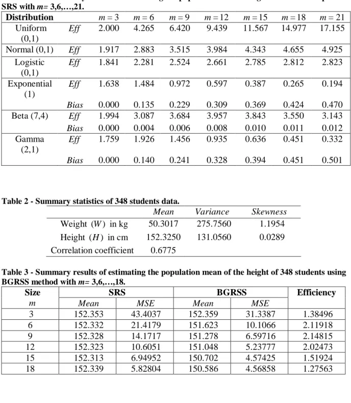
2 ˆ ˆ Var = ˆMSE BGRSSO BGRSSO E BGRSSO . Results of the efficiency and bias values are given in Table 1. Based on Table 1, we may conclude the following:
(1) Gain in efficiency is obtained by using BGRSS compared to SRS for estimating the population mean for different values of m if the underlying distribution is symmetric about its mean. For example, for m=9, the efficiency of the BGRSS is 6.420 for estimating the population mean of a uniform distribution U(0,1). (2) When comparing the efficiencies obtained for the symmetric distributions
considered in this study, the BGRSS is most efficient for estimating the mean of the uniform distribution.
(3) For asymmetric distributions considered in this study, the BGRSS mean estimator has a small bias. For example, if the distribution is B(7,4) with sample size
9 =
m , the efficiency of BGRSS is 3.684 with bias 0.006.
6.
Example for real data set
In this section, a collection of a real data set is used to illustrate the BGRSS for estimating the population mean. These data consists of height (H), and the weight (W) of 348 students. Table 2 contains the summary statistics of the data. We will show how to use the RSS and BGRSS to estimate the mean of the students height based on their weight. It is known that the coefficient of skewness should be close to zero for symmetrically distributed data. But since the coefficient of skewness of the weight and height are 1.1954 and 0.0289, respectively, so that these data are asymmetrically distributed.
To illustrate the RSS and BGRSS methods, we first fix the values of height (H) and do the ranking based on the values of the weight (W). Let k =2, then m=6. For estimating the mean of height consider the following steps:
Step 1: Randomly select 6 independent simple random samples each of size 6 ordered pairs ) , (W H as: Set 1:{(47, 159),(35, 146),(60, 145),(37, 144),(61, 173),(34, 139)} Set 2:{(33, 146), (36, 137), (52, 170), (48, 160), (73, 162), (62, 165)} Set 3:{(54, 160), (56, 165), (39, 151), (37, 155), (55, 147), (46, 160)} Set 4:{(40, 148), (68, 164), (51, 156), (36, 149), (60, 160), (95, 162)} Set 5:{(40, 154), (54, 156), (33, 141), (34, 141), (37, 142), (41, 158)} Set 6:{(50, 158), (56, 166), (87, 155), (37, 144), (40, 138), (49, 163)}.
Step 2: For each set in Step 1, rank the pairs within each set based on their weight (in bold) from the lowest to highest as shown below:
Set 1: (34,139),(35,146),(37,144),(47,159),(60,145),(61,173)} Set 2: (33,146),(36,137),(48,160),(52,170),(62,165),(73,162)} Set 3: (37,155),(39,151),(46,160),(54,160),(55,147),(56,165)} Set 4: (36,149),(40,148),(51,156),(60,160),(68,164),(95,162)} Set 5: (33,141),(34,141),(37,142),(40,154),(41,158),(54,156)} Set 6: (37,144),(40,138),(49,163),(50,158),(56,166),(87,155)}
Step 3: Now, we will consider the SRS, RSS and BGRSS as:
1. Under SRS, we have 6 estimates of the mean. Let ˆH,SRSi be the mean of the ith set
1,2,...,6) = (i . So we have: 151 = ˆH,SRS1 , ˆH,SRS2 =156.66, ˆH,SRS3 =156.33, ˆH,SRS4 =156.5, ˆH,SRS5 =148.66, 154, = ˆH,SRS6
2. Under RSS method, from the ith set, select and measure the height corresponding to the ith ordered weight values. The six RSS height are: 139,137,160,160,158 and 155. Hence, the RSS estimator of the mean is given by:
151.5 = 6 909 = 6 155 158 160 160 137 139 = ˆH,RSS
3. Under BGRSS, the lowest ranked units are measured from the first two sets, the median is measured from the third and fourth sets and largest ranked units are measured from the last two sets. Thus, height values considered are: 139, 146, 157.5, 158, 156, 155. The mean height can be estimated using BGRSS as:
151.92. = 6 911.5 = 6 155 156 158 157.5 146 139 = ˆH,BGRSS
of ˆH,SRS and ˆH,BGRSS. From Table 3, the estimated mean is found to be close to the real value of the population mean. Also, we can see that the BGRSS method is more efficient than the SRS for estimating the population mean of the height.
7.
Summary
A gain in efficiency is obtained using BGRSS for estimating the population mean. It is found that BGRSS is more appropriate for estimating the population mean of symmetric distributions than asymmetric distributions considered in this study. Thus, it is recommended to use BGRSS for estimating the population mean of symmetric distribution, also for estimating the mean of symmetric distributions when the sample size is small since the bias is very negligible.
Appendix: Tables
Table 1 - The efficiency values for estimating the population mean using BGRSS with respect to SRS with m= 3,6,…,21. Distribution m=3 m=6 m=9 m=12 m=15 m=18 m=21 Uniform (0,1) Eff 2.000 4.265 6.420 9.439 11.567 14.977 17.155 Normal (0,1) Eff 1.917 2.883 3.515 3.984 4.343 4.655 4.925 Logistic (0,1) Eff 1.841 2.281 2.524 2.661 2.785 2.812 2.823 Exponential (1) Eff 1.638 1.484 0.972 0.597 0.387 0.265 0.194 Bias 0.000 0.135 0.229 0.309 0.369 0.424 0.470 Beta (7,4) Eff 1.994 3.087 3.684 3.957 3.843 3.550 3.143 Bias 0.000 0.004 0.006 0.008 0.010 0.011 0.012 Gamma (2,1) Eff 1.759 1.926 1.456 0.935 0.636 0.451 0.332 Bias 0.000 0.140 0.241 0.328 0.394 0.451 0.501
Table 2 - Summary statistics of 348 students data.
Mean Variance Skewness
Weight (W) in kg 50.3017 275.7560 1.1954 Height (H) in cm 152.3250 131.0560 0.0289 Correlation coefficient 0.6775
Table 3 - Summary results of estimating the population mean of the height of 348 students using BGRSS method with m= 3,6,…,18.
Size SRS BGRSS Efficiency
m Mean MSE Mean MSE
3 152.353 43.4037 152.359 31.3387 1.38496 6 152.332 21.4179 151.623 10.1066 2.11918 9 152.328 14.1717 151.278 6.59716 2.14815 12 152.323 10.6051 151.048 5.23777 2.02473 15 152.313 6.94952 150.702 4.57425 1.51924 18 152.339 5.82804 150.586 4.56858 1.27563
References
Al-Saleh M. F. and Al-Omari A. I. Multistage ranked set sampling. Journal of Statistical Planning and Inference. 2002;102:273--286.
Dell T. R., and Clutter J. L. Ranked set sampling theory with order statistics background. Biometrika. 1972;28:545--555.
Jemain A. A., and Al-Omari, A. I. Double percentile ranked set samples for estimating the population mean. Advances and Applications in Statistics. 2006a;6(3):261--276.
Jemain A. A. and Al-Omari A. I. Double quartile ranked set samples. Pakistan Journal of Statistics. 2006b;22(3):217--228.
McIntyre G. A. A method for unbiased selective sampling using ranked sets. Australian Journal of Agricultural Research. 1952;3:385--390.
Muttlak H. A. Investigating the use of quartile ranked set samples for estimating the population mean. Journal of Applied Mathematics and Computation. 2003a;146:437--443.
Muttlak H. A. Modified ranked set sampling methods. Pakistan Journal of Statistics. 2003b;19(3):315--323.
Muttlak H. A. Median ranked set sampling, Journal of Applied Statistical Sciences. 1997;6(4):577--586.
Ozturk O. and Deshpande J.V. Ranked Set Sample nonparametric quantile confidence intervals. Journal of Statistical Planning and Inference. 2006;136:570--577.
Samawi H, Abu-Dayyeh W and Ahmed S. Extreme ranked set sampling, The Biometrical Journal. 1996;30:577--586.
Takahasi K., and Wakimoto K. (1968). On the unbiased estimates of the population mean based on the sample stratified by means of ordering. Annals of the Institute of Statistical Mathematics. 1968;20:1--31.