Double Median Ranked Set Sample: Comparing To Other Double Ranked Samples For Mean And Ratio Estimators

(1)

Volume 1 | Issue 2

Article 52

11-1-2002

Double Median Ranked Set Sample: Comparing

To Other Double Ranked Samples For Mean And

Ratio Estimators

Hani M. Samawi

Sultan Qaboos University, Sultanate of Oman

Eman M. Tawalbeh

Yarmouk University, Jordan

Follow this and additional works at:

http://digitalcommons.wayne.edu/jmasm

Part of the

Applied Statistics Commons

,

Social and Behavioral Sciences Commons

, and the

Statistical Theory Commons

This Regular Article is brought to you for free and open access by the Open Access Journals at DigitalCommons@WayneState. It has been accepted for inclusion in Journal of Modern Applied Statistical Methods by an authorized administrator of DigitalCommons@WayneState.

Recommended Citation

Samawi, Hani M. and Tawalbeh, Eman M. (2002) "Double Median Ranked Set Sample: Comparing To Other Double Ranked Samples For Mean And Ratio Estimators,"Journal of Modern Applied Statistical Methods: Vol. 1: Iss. 2, Article 52.

DOI: 10.22237/jmasm/1036109460

(2)

428

Double Median Ranked Set Sample: Comparing To Other Double Ranked Samples

For Mean And Ratio Estimators

Hani M. Samawi

Department of Mathematics & Statistics Sultan Qaboos University

Sultanate of Oman

Eman M. Tawalbeh

Department of Statistics Yarmouk University

Jordan

Double median ranked set sample (DMRSS) and its properties for estimating the population mean, when the underlying distribution is assumed to be symmetric about its mean, are introduced. Also, the performance of DMRSS with respect to other ranked set samples and double ranked set samples, for estimating the population mean and ratio, is considered. Real data that consist of heights and diameters of 399 trees are used to illustrate the procedure. The analysis and simulation indicate that using DMRSS for estimating the population mean is more efficient than using the other ranked samples and double ranked samples schemes except in case of uniform distribution. Also, using double sampling schemes substantially increase the relative efficiency of ratio estimators relative to their counterpart schemes of one stage samples. Moreover, DMRSS is superior to other double sampling schemes for ratio estimation.

Key words: Double extreme ranked set sample; double median ranked set sample, ratio estimation. Introduction

In many agricultural and environmental studies and recently in human populations, it is common for quantification of a sampling unit to be costly as compared with the physical acquisition of the unit. For example, level of bilirubin in the blood of infants can be ranked visually by observing: a) color of the face, b) color of the chest, c) color of lower part of the body, & d) color of terminal parts of the whole body. Then, as the yellowish goes from i to iv, the level of bilirubin in the blood goes higher (Samawi & Al-Sakeer, 2001). In such circumstances, considerable cost savings can be achieved if the number of quantification is only a small fraction of the number of available units but all units contribute to the information content of the quantification.

Hani Michel Samawi is an Associate Professor of Biostatistics. His areas of research are in bootstrap and resampling methods, ranked set sampling estimators, sampling method, testing hypothesis, estimation, and analysis of biostatistics data. E-mail: [email protected].

Ranked set sampling (RSS) is considered to be a new method of sampling compared with other sampling methods that can achieve this goal. RSS was first introduced by McIntyre (1952). The use of RSS is highly powerful and much superior to the standard simple random sampling (SRS) for estimating some of the population parameters.

As a variation of RSS Samawi et al. (1996) and Muttlak (1997) investigated extreme ranked set sample (ERSS) and median ranked set sample (MRSS) respectively. Samawi and Muttlak (1996 & 2001) used RSS and MRSS to improve the performance of the ratio estimator. Also, Samawi (2001) suggested the double extreme ranked set sampling (DERSS). They showed that ERSS, MRSS and DERSS are more practical than RSS and more efficient at least than SRS for estimating the population mean. Moreover, Al-Saleh and Al-Kadiri (2000) showed that the efficiency of estimating the population mean could be improved even more by double ranked set sampling technique (DRSS). Also, they proved that ranking in the second stage is easier than in the first stage.

In this article, DMRSS is introduced. The properties of DMRSS for estimating the population mean, when the underlying distribution

(3)

is assumed to be symmetric about its mean, are discussed. Also, the performance of DMRSS with respect to the other ranked set samples and double ranked set samples, for estimating the population mean and ratio, is considered.

In Section 2 samples notations and definition and some basic results are introduced . DMRSS scheme and properties are introduced in Section 3. Also, its performance with other sampling schemes will be compared for estimating the population mean. In Section 4, the performance of different double ranked samples schemes will be compared with their counterpart one stage ranked samples for ratio estimation based on the relative efficiency. Illustration of the procedure using real data set with final comments and conclusions is discussed in Section 5.

Sample Notations And Definitions With Some Useful Results

One Stage Sampling Univariate population

For any of RSS, ERSS and MRSS schemes, the procedure can be described by selecting r random sets each of size r from the target population. In the most practical situations, the size r will be 2, 3 or 4. Rank each set by a suitable method of ranking like prior information, visual inspection or by the experimenter. In sampling notation this implies:

11 12 1r 21 22 2r r1 r2 rr 1(1) 1(2) 1(r) 2(1) 2(2) 2(r) r(1) r(2) r(r)

X , X ,

, X

X , X ,

, X

_{after ranking}

X , X ,

, X

X , X ,

, X

X , X ,

, X

X , X ,

, X











_{ →}









































(2.1)

where Xji denotes the i-th observation in the j-th set and Xj(i) the i-th ordered statistic in the j-th set.

1) If only

X

₁₍₁₎

,

X

₂₍₂₎

,...,

X

_r₍_r₎, quantified by obtaining the element with smallest rank from the

first set, the second smallest from the second set, and so on until the largest unit from the r-th set is measured. Then, this represents one cycle of RSS. We can repeat the whole procedure m times to get a RSS of size n = mr. (See Takahasi and Wakimoto, 1968.)

2)Similarly, as in Samawi et al. (1996), we have two cases: In case of r is even, and if only RSS,

( )

X

( )

X

( )

X

( )

X

11k

,

2r k

,

…

,

r−11k

,

r rk,

k=1,2,…,m, quantified, then this will denote the

ERSSE . In case of r is odd, and if only

( )

X

( )

X

( )

X

( )

X

k r k r rk r r k 2 1

,

2 1 1 1

…

₋ + ,

k=1,2,…,m, quantified, then this will denote the ERSSO.

3) Again, similar to Muttlak (1997), we have two cases: In case of r is odd, and if only

, ..., m

,

, k

X

,

X

r k r r k

1

2

21 21 1_ +_

…

_ + _

=

,

quantified, then this will denote the MRSSO. In

case of r is even, select for measurement from the first

2 r

samples the

( )

2r -th smallest unit and from

the last

2 r

samples select the











 +

1

2 r

-th smallest unit. This will be denoted by MRSSE (i.e.

( )

r r r r r 1₂k _{2 2}k ₂ 1₂ 1 k r r 1 k 2 , , , , X X X ,_X , k 1, 2, ..., m + + + = … … ).

For bivariate population

Samawi and Muttluk (1996) modified the above procedure in case of bivariate distributions to estimate the population ratio. The procedure is described as follows:

First choose r2_{independent bivariate}

elements from a population, with bivariate distribution function F(x, y). Rank each set with respect to one of the variables Y or X. Suppose ranking is on variable X. Apply the same procedures as in case of univariate population but for each measured unit from the X’s, the associated unit from the Y’s is measured too. This may be repeated m times to get a bivariate sample of size n = rm.

(4)

In sample notation:

1) The sample {

(

_X

_i_{( )}_i _k

,

_Y

_i_{[ ]}_i_k

)

, i=1,2,…,r, k=1,2,…,m} will denote the bivariate RSS.

2) The sample, ( ) ( ) ( ) ( ) 1[1]k 2 r k 2[r ]k 1 1 k r 1[1]k r[r ]k r 1 1 k r r k , ), ( , ), {(X Y X Y ,(X − , Y − ), (X , Y )} … ,

k=1,2,…,m, will denote the bivariate ERSSE and

( ) ( ) ( )

( )

2 r k 1[1]k 2[r]k 1 1 k r 1 r 1 r 1 r k r -1[r]k r ₂ k r ₂ k , Y ), ( , Y ), {(X X , (X ₋ , Y ), (X + , Y _ + _ )}   … ,

k=1,2,…,m, will denote the bivariate ERSSO.

1) Similarly,

( )

(

_i r 1_k _i r 1_k

)

2

,

2

: i

1, 2 ,

,

X

Y

r a n d k

1, 2 ,

,m

+  +     



₌











₌







…

2) will denote the bivariate MRSSO

and

( )

(

)

(

( )

)

( )

(

)

r r r r r r 1₂ k 1 ₂ k _{2 2} k _{2 2} k r ₁ r _{1 k} r ₁ r ₁ 2 2 2 2

,

X

Y

X

Y

,

_X

,

_Y

              + + + __ + __

…

( )

[ ]

(

X

,

Y

)

,

_r r _r r ₁ 2 1 2

,

…

+ + , k=1,2, …, m will denote the bivariate MRSSE.

Double Ranked Samples (Two Stage Sampling) 1) Al-Saleh and Al-Kadiri (2000) introduced DRSS procedure as follows:

1. Identify r3 elements from the target population and divide these elements randomly into r sets each of size r2 elements.

2. Use the usual RSS procedure on each set to obtain r RSS each of size r.

3. Employ again the RSS procedure in Step 2, to obtain the DRSS of size r. 4. We may repeat steps 1-3 m times to obtain a sample of size n = rm.

In sampling notations, after ranking each sample separately in each subset, we get:













) 1 ( ) ( ) 1 ( ) 2 ( ) 1 ( ) 1 ( ) 1 ( ) ( 2 ) 1 ( ) 2 ( 2 ) 1 ( ) 1 ( 2 ) 1 ( ) ( 1 ) 1 ( ) 2 ( 1 ) 1 ( ) 1 ( 1 k r r k r k r k r k k k r k k

X

…

,…,













) ( ) ( ) ( ) 2 ( ) ( ) 1 ( ) ( ) ( 2 ) ( ) 2 ( 2 ) ( ) 1 ( 2 ) ( ) ( 1 ) ( ) 2 ( 1 ) ( ) 1 ( 1 r k r r r k r r k r r k r r k r k r k r r k r k

X

…

, (2.2)

k=1,2,…,m , where

X

_i(_{( )}l_i)_kis the i-th ordered observation in the l-th set in the i-th sample in the

k-th cycle. Use RSS scheme on each subset

separately, we get ( ) ( ) ( ) ( ) ( ) ( )

{

}

( ) ( ) ( ) ( ) ( ) ( )

{

}

1 1 1 1k 1 1 k 2 2 k r r k r r r r k 1 1 k 2 2 k r r k

,

A

X

,

A

X

=

…

.

Then in the second stage, let

_W

_i_{( )}_i_k=i-th smallest observation in

_A

_ik, then {

_W

_i_{( )}_i _k, i=1,2,…,r, k=1,2,…,m} will denote the DRSS. Now let

W

_{( )}₁_k

,...,

W

_{( )}_r_k, k=1, 2, …., m, be a DRSS, with mean and variance of

W

_{( )}_i _kare

µ

_{( )}*_i* and

( )*i*2

σ

, respectively. Al-Saleh and Al-Kadiri (2000) also showed that:

( )** 1

1

i r i

r

µ

∑

=

and ( ) ( )

_







₊

₋

=

_∑

= = 2 * * 1 2 * * 1 2

1 _σ

₍

_µ

₎

σ

r _i i i r i

r

where µ and

σ

2

are the mean and the variance of the population, respectively. Also, it was shown that ranking in the second stage is easier than in the first stage.

2) DERSS is an extension to ERSS procedure by

Samawi (2001). The procedure is just similar to that for DRSS, but taking ERSS instead of RSS in the first and in the second stage. Implies that

(5)

( )

,

( )

,

( )

,

...,

( )

,

k

1,

2,

....,

m

}

{

W

₁₁_k

W

₂_r_k

W

₃₁_k

W

_r_r_k

=

d enotes DERSSE. The case when r is odd is similar.

For more about RSS see for example Kaur et al.,

(1995) and Patil et al. (1999). Double Median Ranked Set Sample

In this Section a modification to MRSS, namely double median ranked set sample (DMRSS) is introduced. The properties of this scheme for estimating the population mean, which is considered to be finite, is discussed when the underlying distribution function is assumed to be symmetric. Also, some numerical and theoretical comparisons with SRS, RSS, MRSS, ERSS, DERSS and DRSS are included.

Sample Notation and Definitions

For each cycle k=1,2,…,m (m= number of cycles), assume a simple random sample, of size r3, is selected from a target population with c.d.f. F(x) and p.d.f. f(x), where F(x) is assumed to be symmetric and absolutely continuous, with mean µ and variance σ2_{. Suppose we divided the sample}

independently into r sets of data where each set contains r samples, each of size r. Two cases are considered:

Case 1:From (2.2) and when r is odd, for the k-th cycle, get r2_{ranked samples as in (2.2):}

Take the median ( )

_{( )}

j

k r i X

2+1

from each sample in each set, then the following sets are resulted: A1k=

{ ( )

_{( )}

1 21 1 r k X ₊ , ( )

_{( )}

1 k 21 r 2 X ₊ , ..., ( )

_{( )}

1 21 k r r X ₊ }, A2k= { ( )

( )

2 21 1 r k

X

₊ _, ( )

_{( )}

2 21 2 r k X ₊ , ..., ( )

_{( )}

2 21 k r r X ₊ }, ..., Ark= {

X

( )

_{( )}

rr _k 21 1 + ,

( )

( )r k r X 21 2 + , ...,

( )

( )r k r r X 21 + }.

These sets are the first stage MRSS samples. The second stage MRSS or double MRSS is the set of medians of A1k, A2k, …, Ark. Define

( )

k r

W

21 1 + = med(A1k),

( )

k r

W

21 2 + = med(A2k), …,

W

r

( )

r k 2+1 = med(Ark), then the sample {W

( )

r _k

21 1 + ,W

( )

r k 21 2 + , …,

( )

r k r W 21 + }, k=1,2,…,m is denoted by DMRSSO.

The sample mean using DMRSSO is given by

=

∑∑

_{( )}

= = + m k r i ir k DMRSS

W

rm

W

O 1 1 ₂1

1

. (3.1)

Case 2: When r is even, for the k-th cycle, after ranking each sample in each set, as in Case 1, divide the r sets in (2.2) in half to two independent sets. From the first

2

r _{sets take the (}

2

r _)-th

smallest unit from each sample and from the last

2

r _{sets take the (}

2

r _{+1)-th smallest unit from each}

sample, that is, we will get the following sets:

( )

{

X

}

A

k r _k r _k _r r_k 1 2 1 2 2 1 2 1 1

=

,

…

,

( )

{

X

}

A

k r r k r k r k 2 2 2 2 2 2 2 1 2

=

,

…

,

,…,

( )













=

2 2 2 2 2 2 2 1 2

,

r k r r r k r r k r k r

X

A

…

,

( )













=

+₊ +₊ +₊1 2 1 2 1 2 1 2 2 1 2 1 2 1 1

,

r k r r r k r r k r k

X

B

…

,

( )









=

+₊ +₊ +₊2 2 1 2 2 2 1 2 2 2 2 1 2 1 2

,

r k r r r k r r k r k

X

B

…

,…

( )









=

₊ ₊ r ₊ k r r r k r r k r k r

X

B

1 2 1 2 2 1 2 1 2

,

…

,

k=1,2,…, m. This is the first stage. Again from each Aik take the ( 2

r

)-th smallest units, while from each Bik take the ( 2

r +1)-th smallest unit as follows:

-

th

2 the

2













=

     

r

W

k r i ordered statistic from Aik, i=1, 2,… , 2 r , k= 1, 2, …, m and th -1 2 the 1 2       + =       + r W k r

i ordered statistic from

Bik, i=1, 2, … , 2

r

(6)

sample

( )

r r r r 1 k 2 k k 2 2 2 2 r r r r 1₂ 1 k 2₂ 1 k _{2 2} 1 k

,

, ,

,

W

,

, ,

W

+ + +

…

,

k=1,2,…,m denotes DMRSSE. The sample mean

using DMRSSE is given by

∑

_













∑

+

∑

=

= = _ _ = _ + _ m k r i r i i r k k r i E DMRSS

W

rm

W

1 2 1 2 1 ₂ 1 2

1

. (3.2)

To study the properties of DMRSSO and

DMRSSE, next we derive the distribution

functions of

_{( )}

21 + r W ,

_{( )}

1 2 2

and

+ r r

W

respectively

and some of their properties.

Distribution Function and Properties of DMRSS Case 1:When r is odd. To find the distribution of

( )

r k i

W

2+1 , i=1,2, …, r say

G

_{( )}

_r

( )

w

21 + , first the distribution of ( )

_{( )}

j k r i

X

21 + say

F

( )

r

( )

x

2 1 + is given by

( )

( ) ( )

( )

(

)

(

( )

)

( )

r 1 2 r 1 r 1 2 2 x _r! F x f(t) r 1 _! r 1 _! 2 2 F t 1 F t d t + − − = _∫ − − − ∞ − (3.3)

(see Arnold, et al. 1992). Let u = F(t), then

( )( )

_{( )( )}

( )

(

)

( )

(

₂1, ₂1

)

, 1 ! ! ! ₂1 21 ) ( 0 ₂1 ₂1 21 + + = − ∫ = ₋ ₋ − − + r r I du u u r x F x F r r x F r r r (3.4) which is the usual incomplete beta function. Hence, ( )

_{( )}

j k r

X

21 1 + ,

( )

( )j k r

X

21 2 + , …,

( )

( )j k r r

X

2+1 , are independent and identically distributed (i.i.d.) with incomplete beta

_I

_F₍_x₎

(

r+₂1

,

r+₂1

)

distribution. Now

from the definition of DMRSSO, the p.d.f. of

( )

r k i

W

21 + will be

( )

( ) ( ) ( )

( )

(

)

( )

(

)

( )

r 1 2 r 1 r 1 _{r 1} _{r 1} 2 2 2 2 r 1 2 r 1 r 1 2 2

r!

g

w

F

w

!

1 F

w

f

w

− + + ₋ ₋ − + +

=

−

=

( )( )

(

( )

(

)

(

)

( )

(

( )

)

(

)

( )

2 _{r 1} 2 r ! r 1 r 1_, r 1 r 1_, F w _{2 2} F(w) _{2 2} r 1 _! r 1 _! 2 2 r 1 2 1 I I f w . F w 1 F w − + + + + − − −   −     × − × (3.5) Let _{( )}

(

, ₂1

)

, then 21 + + = r r t F

I

s the c.d.f. of

( )

r k i

W

2+1 is

( )

_{( ) ( )}

( )

(

)

( )

(

,

)

.

1 !

!

21 21 21 21 21 21 0 ₂1 ₂1 2 1 + + + + − − − −       +

=

−

∫

=

r r r , r w F r r r r

I

ds

s

r

w

G

I IF w r (3.6) Note that,

_{( )}

,

_{( )}

,

_{( )}

21 21 2 21 1r k

W

r k

W

r r k

W

₊ ₊

…

₊ , k=1 ,2

,…, m are i.i.d. with the (3.6 ) distribution function.

Case 2: Distribution function of

_{( )}

2 r i

W

and

_{( )}

1 2+ r i

W

, i=1, 2, …,

2 r

when r is even.

Recall the assumption that the MRSS is based on a

simple random sample of size r3_{with the}

symmetric and i.i.d. distribution function F(x). Distribution function of

_{( )}

2 r i

W

Using the same steps as in case 1, the p.d.f. and c.d.f. of k r i

W

      2 , i =1, 2, …,

2 r

, will be respectively

(7)

( )

( ) ( )

( )

(

)

( )

r 1 2 r r ( ) ₂ 2 r 2 r 2

r!

g

w

F

w

r

_!

r

_{1 !}

2

2 1 F

w

_f

r

2

−

=

−













( ) (

)

( )

(

)

(

( )

)

( )

r 2 ₁ 2 F(w) r r 2 2 r 2 F(w) r ₁ r 2 2

r !

r r

_,

₁

I

!

1 !

2 2

r r

1 _I

,

1 2 2

f w

1 F w

F w

− −



_{ }

_

_

=



_

_{ }

_

_

+

_

−











₋



₊





_



_







×

−

×

(3.7) and

( )

( ) (

)

( )

_{( )}

( )

(

)

( )

( ) r 2 r r_, ₁ F w _{2 2} _r r 1 2 ₂ r r 2 2 0 r r_, ₁ IF w 2 2

G

w

I

r!

_{1 s}

_{d s}

s

!

1 !

r r

,

1 .

I

_{2 2}

 ₊      ₋  ₊     

=

−





=

_

+

_





∫

(3.8)

Note that, the

_{( )}

k r i

W

2 , i =1, 2, …, ₂r, k=1, 2, …, m are i.i.d. with (3.7) distribution function. Similarly, the p.d.f. and c.d.f. of

_{( )}

k r i

W

2 , i=1, 2 , …,

2 r

, k=1, 2, …, m, say,

g

( )

r ₁

( )

w

2+ and

( )

w

G

_r 1 2+ respectively are,

( )

( ) ( )

( )

(

)

( )

(

)

( )

( )( )

(

( )

)

( )

(

)

( )

(

)

( )

(

( )

)

( )

r 2 r 1 r 1 2 2 r 1 2 r 1 r ₁ 2 2 2 _r 2 r! r _1,r F(w) r _! r _{1 !} 2 2 2 2 r 1 2 r _1,r F(w) 2 2 r 1 2 r 2 r! w F w g r _! r _{1 !} 2 2 w f 1 F w I 1 I F w 1 F w f w         + + − + + + − − + − = − −   =     × − × − (3.9) and,

( )

( ) (

)

( )

_{( )}

( )

(

)

( )

( ) r 1 2 r _1,r F w 2 2 _r r 1 2 2 r r 2 2 0 r _1,r IF w 2 2

G

w

I

r!

_{1 u}

_du

u

!

1 !

r

_1,

r

_.

2

2 I

+  ₊      −  ₊     

=

−





=

_

+

_





∫

(3.10) Hence, k r

W

      +1 2 1 ,

W

_ +1r _k 2 2 , …,

W

r_ +1r _k 2 2 , are i.i.d. with the distribution function as in (3.10). However, k r

W

      2 1 ,

W

2_₂r_k, …,

W

₂r_r₂_k,

W

1_ +1r₂ _k, k r

W

      +1 2 2 , …,

W

r_ +1r _k 2 2

, are independent but not identically distributed.

DMRSS for Estimating the Population Mean The following results are stated and proved in the Appendix. Using DMRSS when the underlying distribution is assumed to be

symmetric.

W

DMRSS_O

and

W

DMRSSE are

unbiased estimators for µ, and

(

)

(

)

n

2

σ

≤

_X

W

DMRSS

Var

MRSS

Var

, where

(8)













₊

=

∑∑

= = + = = + m k r i k r i m k r i k r i k r i MRSS

X

n

X

n

X

1 1 ₂ ) 1 ( 1 2 / 1 (₂) (₂ 1)

odd

is

r

if

,

1 even

is

r

if

,

)

(

1

(see the Appendix for Theorem 1, Lemma 1 and Theorem 2.

Simulation Study

Based on 5000 replication, a computer simulation is conducted to study the behavior of the efficiency of the sample mean using SRS, MRSS, RSS, ERSS, DERSS and DRSS with respect to DMRSS. Random observations are generated from (1) standard normal distribution (2) Logistic distribution with α =2, β=1 and (3) uniform distribution with θ1 =0, θ2=4. The

performance of the samples means for r=4,5,6 and7 and m=4 and 6 are investigated.

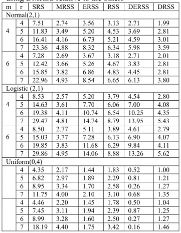
Results of simulation study

The results of these simulations are summarized by the relative efficiency ( the ratio of the variances) of the estimators of the mean. The simulation results are given in Table 3.1.

Table 3.1 shows that estimating the population mean using DMRSS is substantially more efficient than SRS, MRSS, ERSS and RSS. Comparing the sample mean using MRSS with the sample mean using DMRSS, our simulation confirms the results of Theorem 3.2 for the three distributions. Comparing the efficiency for estimating the population mean using DMRSS relative to DERSS, there is a notable difference between them according to the distributions. The best performance was in case of logistic distribution. In normal distribution, the relative efficiency was slightly lower than in logistic distribution.

Clearly in case of uniform distribution, estimating the population mean using DERSS is more efficient than using DMRSS. Also, the population mean estimator using DMRSS is more efficient than the population mean estimator using DRSS, when the underlying distribution is assumed to be symmetric.

Regarding the sample size r, the relative efficiency of the population mean estimators, using DMRSS with respect to any of the other

Table 3.1: The efficiency of the mean estimators using DMRSS relative to the others

m r SRS MRSS ERSS RSS DERSS DRSS Normal(2,1) 4 7.51 2.74 3.56 3.13 2.71 1.99 5 11.83 3.49 5.20 4.53 3.69 2.81 6 16.41 4.16 6.73 5.21 4.59 3.01 4 7 23.36 4.88 8.32 6.34 5.98 3.59 4 7.28 2.69 3.67 3.18 2.71 2.01 5 12.42 3.66 5.26 4.67 3.83 2.81 6 15.85 3.82 6.86 4.83 4.45 2.81 6 7 22.96 4.93 8.54 6.65 6.13 3.80 Logistic (2,1) 4 8.53 2.57 5.20 3.79 4.54 2.80 5 14.63 3.61 7.70 6.06 7.00 4.08 6 19.38 4.11 10.74 6.54 10.25 4.35 4 7 29.47 4.81 14.74 8.79 13.95 5.43 4 8.50 2.77 5.11 3.89 4.61 2.79 5 15.03 3.77 7.28 6.13 6.90 4.07 6 19.85 3.83 11.68 6.29 9.84 4.11 6 7 29.86 4.95 14.06 8.88 13.26 5.62 Uniform(0,4) 4 4.35 2.17 1.44 1.83 0.52 1.00 5 6.82 2.97 1.89 2.29 0.81 1.21 6 8.95 3.34 1.70 2.58 0.26 1.27 7 11.75 4.00 2.10 3.10 0.68 1.35 4 4.46 2.20 1.45 1.78 0.50 1.04 5 7.45 3.11 1.94 2.39 0.87 1.25 6 8.99 3.28 1.60 2.50 0.27 1.27 7 18.19 4.40 1.75 3.42 0.16 1.46

previous sampling techniques, increases as r increases. While considering the cycle size m, the relative efficiency for the sample mean using DMRSS relative to the other sampling schemes is not affected by the value of m.

Ratio Estimators

Frequently the quantity that is to be estimated from a bivariate random sample is the ratio of two means of two correlated variables, say X and Y, which both vary from unit to unit. For example, in a household survey, the average expenditure on cosmetics per adult female, and the average number of hours per week spent watching television for child aged 10 to 15.

Examples of this kind occur frequently when the sampling unit (the household) comprises a group or cluster of elements and our interest is in the population mean per element. Also, the ratio estimation method is used to obtain increased precision of estimating the population mean or total by taking advantage of the correlation between an auxiliary variable X and the variable of interest Y. In this paper, we assume that the

(9)

[ ]

∑ ∑

=

i k

Y

i k

rm

Y

1

bivariate random variable (X,Y) has symmetric marginal distributions.

Ratio Estimator Using SRS

Let the bivariate random variable (X,Y) has c.d.f. F(x,y) with means

µ

_x

and

µ

_y,variances

σ

2

_and

2

y

x , and correlation coefficient ρ, then

x y

R

µ

=

will denote the population ratio. Using a simple bivariate random sample from F(x, y), the estimator of R is given by:

X

Y

R

_SRS

=

(4.1)

where X and Y are the means of X and Y

respectively.

Hansen et al.(1953) showed that the variance of

R

_SRS can be approximated by

(

SRS

)

≅ _Vx +Vy − VxVy_ n R R Var 2 2 2 2

ρ

_, (4.2) where x x x V

µ

σ

= , y y y

V

µ

σ

=

,

(

)

(

)

(

)

y x y x

Y

X

E

σ

µ

ρ

=

−

and n= rm.

Ratio Estimator Using RSS

Samawi and Muttlak (1996) showed that the ratio estimator using RSS when ranking is on

the variable X, is [ ] ( )r r RSS

X

Y

R

2

=

, where [ ]

∑∑

_{[ ]} = =

=

m k r i iik r

Y

n

Y

1 1

1

, ( )

∑∑

_{( )} = =

=

m k r i iik r

X

n

X

1 1

1

and the variance is given by

(

)

2 R S S 2 2 x y x y r r ₂ r ₂ x ( i ) y [ i ] _{x ( i )y [ i} i 1 i 1 i 1 2 2 x y x y R V a r R n V V 2 V V T T T _] _, m 2 n n n = = = ≅  + − ρ       _∑ _∑ _∑  × ₋  ₊ ₋    _µ _µ _{µ µ}         (4.3) where

x

i

x

T

=

µ

₍_i₎

−

µ

)

(

,

T

y[i]

=

µ

y[i]

−

µ

y and

)

)(

(

₍₎ _[_] ] [ ) (i yi xi x yi y x

T

=

µ

−

µ

−

µ

.

As demonstrated by Samawi and Muttluk (1996), that ranking on X is more efficient than ranking on Y in ratio estimation in terms of variance, therefore we introduce only the case where ranking on the variable X is assumed to be without errors. In the next subsections, we will introduced and study the performance of ratio estimators using the double ranked samples discussed in the pervious sections.

Ratio Estimation Using DRSS

Using the notation of Section 2.3, the second stage a subsample of size n=rm,

( )

,

1 ,

2 ,

,

1 ,

2 ,

,

}

{

W

iik

i

=

…

r

k

=

…

m

is selected.

Also, in the second stage, for each

W

_i

_{( )}

_i _k measure (quantify) the associated value of the random variable Y. The bivariate DRSS

( ) [ ]

(

)

{

W

_i_i_k

, Y

_i_i_k

:

i

=

1 ,

2 ,...,

r

,

k

=

1 ,

2 ,...,

m

}

is measured, where

W

_i

_{( )}

_i _k as defined above, and

[ ]i k i

Y

is the corresponding value of Y obtained

from the i-th RSS sample in the k-th cycle. Now, let

_µ

_x**

=

W

_and

_µ

*_y*

=

Y

,

where

=

∑ ∑

_{( )}

i k

W

i k

rm

W

1

, and then the

estimate of population ratio R using DRSS is given by

(10)

.

W Y

R_DRSS =

(4.4)

By using Taylor expansion and assuming large population size, it is easy to show that

(

)













+

=

n

O

R

E

x y DRSS

1 µ

µ

,

and the variance of

R

_DRSS will be approximated by

(

)

( ) 2 D R S S 2 2 x y x y r r r * * 2 * * 2 * * w ( i ) y [ i ] w i y i i 1 i 1 i 1 2 2 y x x y

R

V a r R

n

2 m

V

V V

T

2 n

n

    = = =

≅



+

− ρ

−

























+

−









µ





_

_µ

µ

_





_

_







∑

(4.5) where 2

and

2

V

x y as in equation (4.2).

Ratio Estimation Using DMRSS

Using similar modification for bivariate case, and assuming that ranking is on variable X in the two stages. Then as in section 2, (W1(s)k,Y1[s]k),

(W2(s)k ,Y2[s]k), …,(Wr(s)k ,Yr[s]k) k=1, 2, …,m will

denote the bivariate DMRSS where s is (

2 r

) for the first

2 r

units and (

1

2 +

r

) for the last

2 r

units in case when r is even and (

2

1 +

r

) when r is odd. Wi(s)k is the s-th smallest X unit in the k-th cycle of

the i-th bivariate MRSS in the first stage and Yi[s]k

is the corresponding Y observation in the k-th cycle of the i-th bivariate MRSS.

Two cases are considered here:

Case(1): When r is odd, the estimate of the

population ratio R using DMRSSO is defined by

O O DMRSS

W

R

Y

O

=

, where ,

1 ,

1

] 21 [ ) 21 (

=

∑∑

=

₊ ₊ k i i r k O k i i r k O

Y

mr

Y

W

mr

W

(4.6)

Again, by using Taylor expansion we have

(

)













+

=

n

O

R

E

x y MDRSSo

1 µ

µ

and ( ) ( )

(

)

D M R S S o 2 * * 2 * * 2 * * * * w s y s W ( s )Y [ s ] w s y s

V a r(

_R

)

R

₂

_,

V

m r

r

1 w h e re s

2

       

≅

+

− ρ

+

=

(4.7) ( ) ( ) [ ] [ ]₂ 2 2 2 2 2

µ

σ

V

,and

µ

σ

V

y ** s y ** s y x ** s w ** s w

=

.

Case(2): When r is even, the estimate of the

population ratio R using DMRSSE is given by

W

Y

E E E DMRSS

R

=

,

(4.8) where, ( ) r E _{i s k} k i 1 r 2 r 2 r r i k i 1 k k i 1 ₂ i 1 ₂ 1 W W mr 1 _W _W mr =    ₊     = _{ } = _ _ =     = +    

∑∑

∑ ∑

∑

and r E _{i s k} k i 1 r 2 r 2 r r i k i 1 k 2 2 k i 1 i 1

1 Y

Y

mr

1 Y

Y

.

mr

    =    ₊         = =

=





=

_

+

_





∑∑

∑ ∑

∑

Again by using Taylor expansion, and

assuming symmetric underlying distributions then

(

)













+

=

n

O

R

E

x y MDRSSE

1 µ

µ

and

(11)

(

)

( ) ( ) ( ) E r r r r 2 2 1 2 2 y 2 DMRSS x ** ** ** 2 ** 2 w y w 1 y 1 y s w s 2 2 x y y x

Var

mr

R

σ

µ

  +  +        

≅



₊





₊

₋















µ

σ

µ µ

µ

( ) ( )

(

)

2 ** 2 ** 2 ** ** w s y s W(s)Y[s] w s y s R _V _V ₂ _V _V mr       = + − ρ (4.9) where _{( )} ( ) _{[ ]} ₂[ ] 2 2 2 2 2

µ

σ

V

µ

σ

V

y ** s y ** s y x ** s w ** s w

=

,

=

and s can be either











 +

1

2 or

2 r

r

since

( )

σ

( )

σ

[ ]

σ

[ ]

σ

** 1 2 * * 2 * * 1 2 * * 2

and

+ +

=

_wr _yr _yr r w .

Ratio Estimation Using DERSS

Assume without loss of generality that r is even. The case when r is odd is similar and it will be indicated in the numerical results only. Also assume ranking is on variable X. Let

( )

(

)

(

( )

)

( )

(

)

(

( )

)

11 k 11k 2 r k 2 r k 3 1 k 3 1k r r k r r k

W ,Y

, W

,Y

,

W ,Y

, ..., W ,Y

                be the bivariate

DERSS

(see Samawi, 2001). This set of bivariate observations is independent but not identically distributed.

The estimate of the population ratio R using

DERSS

is given by DERSS DERSS DERSS

W

Y

R

ˆ

=

, (4.10) where ( ) ( ) ( ) ( )

(

)

DERSS i 1 k i r k k i odd i even r 2 r 2 2 i 1 1 k 2 i r k i 1 i 1 k 1 W W W m r 1 _W _W m r = − =   = _ + _   = +

∑ ∑

∑

∑ ∑

∑

, 1 r D E R S S r 2 2 i 1 1 k 1 k i 1 r 2 2 i 1 k r k i 1

Y

,

2 Y

1 Y

,

m

r 2

Y

1 a n d Y

m

r 2

        −  _{ }     =         =

+

=





=



_



_









=



_



_





∑ ∑

.

Once again, by using Taylor expansion we have

(

)













+

=

n

O

R

E

x y EDRSS

1 µ

µ

and

(

)

( ) ( )

(

)

( ) ( )

(

)

DERSS 2 ** 2 ** 2 ** ** w 1 y 1 _W(1)Y[1] w 1 y 1 2 ** 2 ** 2 ** ** w r y r W(r)Y[r] w r y r

Var R

R

_V

₂

_V

mr

R

_V

₂

_V

mr

               

≅

+

− ρ

=

+

− ρ

(4.11) where ( ) _{( )} ( ) ( ) ** ** * * w j w j x y j ** ** ** ** y j W(j)Y[j] w j y j y y j w j

,

µ

V

σ

V

ρ

σ

and

µ

σ

               

=

, j=1 or r. Simulation Study

A computer simulation is conducted to study the efficiency of estimating R when ranking is performed on the variable X. Using SRS, RSS, MRSS, ERSS, DRSS, DERSS and DMRSS, bivariate random samples where generated from a bivariate normal distribution with µx=2, µy=4, σx=1, σy=1and ρ=

±

0.9,

±

0.8,

±

0.5.

The performance of the ratio estimate will be investigated for r=4, 5, 6 and 7 and m=4 and 6. The ratios of the population means are estimated from SRS, RSS, MRSS, ERSS, DRSS, DERSS and DMRSS data sets. Using 5000 replications,

(12)

estimates of the means, the mean square errors and the ratio of the mean squrare errors (relative efficiency) for the ratio were computed.

Results of the simulation study

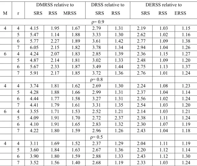
The values obtained by the simulation study are given in Table 4.1. In all cases the simulation showed that the efficiency of estimating R is not affected by the cycle size m, an explanation for this is that m is canceled in the numerator and dominator when relative efficiency is used. The values in the tables vary from a value of m to another because of the simulation variation. When the underlying distribution is N2(2,4,1,1,ρ), Table 4.1 shows that estimating the

population ratio using DMRSS is more efficient

than using SRS, RSS, and MRSS. Also, using DRSS to estimate the population ratio is more efficient than using SRS and RSS, and using DERSS is more efficient than using SRS, RSS and ERSS.

Moreover, using the definition of relative efficiency, the double sampling schemes can be compared with each other. Our simulation indicates that, estimating the population ratio using DMRSS is more efficient than using DRSS

and DERSS. Also, whenever

ρ

increases the

efficiency increases in all cases. Note that negative values of ρ give higher efficiency than the positive values.

Table 4.1 Efficiency of the estimators of R when ranking on X and (X,Y) has N2(4,2,1,1,ρ)

M r DMRSS relative to SRS RSS MRSS DRSS relative to SRS RSS DERSS relative to SRS RSS ERSS ρ= 0.9 4 4 4.15 1.95 1.67 2.79 1.31 2.19 1.03 1.15 5 5.47 1.14 1.88 3.33 1.30 2.62 1.02 1.16 6 5.77 2.27 1.89 3.61 1.42 2.77 1.09 1.38 7 6.05 2.15 1.82 3.78 1.34 2.94 1.04 1.26 6 4 4.24 2.07 1.83 2.85 1.39 2.36 1.15 1.27 5 4.87 2.14 1.81 3.02 1.33 2.48 1.09 1.20 6 5.67 2.33 1.87 3.49 1.44 2.75 1.13 1.37 7 5.91 2.17 1.85 3.72 1.36 2.76 1.01 1.24 ρ= 0.8 4 4 3.74 1.81 1.62 2.69 1.30 2.24 1.08 1.23 5 4.28 1.88 1.66 2.99 1.31 2.37 1.04 1.14 6 4.44 1.77 1.58 3.27 1.31 2.56 1.02 1.24 7 4.41 1.79 1.61 3.31 1.35 2.54 1.03 1.20 6 4 3.55 1.71 1.53 2.52 1.21 2.14 1.03 1.21 5 4.09 1.91 1.70 2.72 2.37 2.38 1.11 1.24 6 4.10 1.91 1.65 2.83 1.32 2.30 1.07 1.19 7 4.22 1.80 1.59 2.96 1.26 2.43 1.04 1.18 ρ= 0.5 4 4 3.11 1.69 1.52 2.37 1.29 2.04 1.11 1.19 5 3.60 1.84 1.63 2.67 1.36 2.20 1.12 1.14 6 3.90 1.80 1.59 2.88 1.33 2.43 1.12 1.30 7 3.52 1.56 1.40 2.68 1.19 2.33 1.03 1.24

(13)

6 4 2.99 1.68 1.52 2.36 1.33 2.01 1.13 1.16 5 3.45 1.67 1.51 2.53 1.23 2.15 1.04 1.10 6 3.66 1.66 1.47 2.85 1.29 2.26 1.02 1.20 7 3.46 1.65 1.46 2.63 1.26 2.29 1.09 1.22 ρ= -0.5 4 4 5.12 2.22 1.99 3.17 1.37 2.55 1.11 1.24 5 6.08 2.40 2.01 3.51 1.38 2.91 1.15 1.34 6 7.67 2.55 2.01 4.14 1.51 2.94 1.07 1.37 7 7.23 2.23 1.96 4.22 1.41 3.23 1.08 1.33 6 4 4.52 2.08 1.78 2.96 1.36 2.39 1.10 1.27 5 5.63 2.39 2.01 3.32 1.41 2.74 1.16 1.34 6 6.93 2.44 2.00 4.17 1.88 3.11 1.09 1.40 7 6.91 2.23 1.95 4.21 1.72 3.09 1.00 1.26 ρ= -0.8 4 4 6.73 2.73 2.37 3.83 1.56 2.89 1.17 1.35 5 8.77 3.15 2.58 4.19 1.51 3.06 1.10 1.29 6 10.31 3.52 2.72 4.97 1.70 3.41 1.17 1.42 7 12.95 3.64 3.03 5.72 1.61 3.83 1.08 1.36 6 4 5.90 2.54 2.19 3.49 1.50 2.71 1.17 1.32 5 9.33 3.12 2.62 4.24 1.42 3.25 1.09 1.27 6 9.07 3.30 2.71 4.42 1.61 3.13 1.14 1.43 7 11.84 3.60 2.79 5.62 1.71 3.72 1.13 1.39 ρ= -0.9 4 4 6.76 2.18 2.43 3.50 1.45 2.72 1.13 1.34 5 11.03 3.84 3.05 4.54 1.58 3.52 1.23 1.36 6 12.91 3.83 3.13 5.20 1.54 3.66 1.08 1.45 7 17.19 4.66 3.56 6.36 1.72 3.99 1.08 1.42 6 4 6.84 2.90 2.46 3.56 1.51 2.78 1.18 1.40 5 10.63 3.69 2.92 4.41 1.53 3.40 1.18 1.36 6 12.82 4.04 3.19 5.17 1.63 3.43 1.08 1.41 7 16.33 4.50 3.50 5.80 1.60 3.77 1.04 1.37

Application To Real Data Set And Conclusions We illustrate the double ranked sample mean estimation procedure using a real data set which consists of the height (Y) and the diameter (X) at breast height of 399 trees. See Platt et al. (1988) for a detailed description of the data set. The summary statistics for the data are reported in Table 5.1. Note that the correlation coefficient is

ρ=0.908.

Table 5.1. Summary Statistics of trees data.

Variable Mean Variance Height (Y) in

feet 52.36 325.14

Diameter (X) in cm

20.84 310.11 In this article, ranking is performed on the variable X exactly measured. However, in practice ranking is done before any actual quantification. Using a set size r = 3 and the cycle size m = 3, we draw bivariate SRS, DRSS, and DMRSS of size 9,

(14)

however DERSS is the same as DRSS in this case. Table 5.2 contains all the above proposed estimators and their estimated variances using the drawn samples.

Table 5.2. Results from the drawn samples. Sample Naïve Estimator of the Diameter (X) 9(Estimated

Variance)* Ratio _Estimator 9(Estimated _Variance)*

SRS 13.57 168.60 2.50 1.036

DRSS 19.39 148.37 2.29 0.633

DMRSS 15.89 131.35 2.15 0.297

Table 5.2 confirms the simulation results. However, this example is just to illustrate the application using the proposed estimators.

Finally, the theortical and simulation results showed that the population mean estimator using DMRSS is an unbiased estimator for the population mean whenever the underlying distribution is assumed to be symmetric. Also, it was shown theoretically that the variance of this estimator is less than the variance of the sample mean using MRSS (the first stage). Although using numerical simulation it was noticed that the sample mean based on DMRSS is more efficient than using other sampling methods (see Table 3.1) with respect to there variances.

Note there are difficulties in selecting the DMRSS because of the similarity of the subjects from the first stage. However, in practice this is not a problem because the number of units we rank in the second stage will not exceed 5.

In ratio estimation using the two stage sampling for different schemes, the estimator of the population ratio of two variables was introduced and the variance in each case was derived. Our numerical study indicated that the two stage sampling is more efficient than the first stage sampling considering the same sampling scheme with respect to their variances.

Comparing the two stage sampling schemes, namely DRSS, DMRSS and DERSS, superiority in efficiency depends on the distribution of the bivariate variable. However, DMRSS was more efficient than DRSS and DERSS when the underlying distribution is the bivariate normal. Moreover, those efficiencies depend on the set size r and the strength of the correlation between X and Y.

References

Al-Saleh, M. F., & Al-Kadiri, M. A. (2000). Double ranked set sampling. Statistics and probability letters, 48(2), 205-212.

Arnold, B. C., Balakrishnan, N., & Nagaraja, H. N. (1992). A first course in order

statistics. New York: John Wiley and Sons, Inc.

Hansen, M. H., Hurwitz, W. N., &

Madow, W. G. (1953). Sampling survey methods

and theorey. Vol. 2. John Wiley and Sons.

Kaur, A., Patil, G. P., Sinha, A. K., & Tailie, C. (1995). Ranked set sampling: an

annotated bibliography. Environmental and

Ecological Statistics, 2, 25-54.

McIntyre, G. A. (1952). A method for unbiased selective sampling using ranked set.

Australian Journal of Agricultural Research, 3,

385-390.

Muttlak, H. A. (1997). Median ranked set sampling. Journal of Applied Statistical Science,

6( 4), 245-255.

Patil, G. P., Sinha, A. K., & Taillie, C. (1999). Ranked set sampling: A bibliography.

Environmental and Ecological Statistics, 6, 91-98. Platt, W. J., Evans, G. W., & Rathbun, S.L. (1988). The population dynamics of a long-lived conifer. The American Naturalist,131, 391-525.

Samawi, H. M. (2001, in press). On double extreme ranked set sample with application to regression estimator.

Samawi, H. M. Ahmed, M. S., & Abu Dayyeh, W. (1996). Estimating the population mean using extreme ranked set sampling.

Biometrical Journal, 38, (5) 577-586.

Samawi, H. M., & Al-Sageer, O. A. (2001). On the estimation of the distribution function using extreme and median ranked set sampling. Biometrical Journal,43(3), 357- 373.

Samawi, H. M., & Muttlak, H. A. (1996). Estimation of ratio using ranked set sampling.

Biometrical Journal, 38 (6), 753-764.

Samawi, H. M., & Muttlak, H. A.(2001). On ratio estimation using median ranked set sampling. Journal of Applied Statistical Science, 10(2), 89-98.

Takahasi, K., & Wakimoto, K. (1968). On unbiased estimates of the population mean based on the stratified sampling by means of ordering.

Annals of the Institute of Statistical Mathematics,

(15)

~

iid

Yang, H.(1980). On the Variance of

median and some other statistics. Bulletin of

Institute Mathematics Academic Simulation, 10,

197-204.

Appendix

Theorem 1: Let X be a random variable with symmetric distribution function F (x)and meanµ, then (a)

g

_{( )}

r

( )

w

2 1 + is symmetric about µ , if r is odd.

(b) Without loss of generality, assume

that

µ

=

0

, then

_W

( )

r

d

_W

( )

r ₁ 2 2

−

+ and hence

0

2

* * 1 * * 2 2

=

+

µ

₊

µ

r r if r is even, where

( )

W

E

( )

W

( )

E

r r r r ₁ 2 * * 1 2 2 * * 2

=

and

µ

+

=

+

µ

. Proof: (a) Because

f

_r

( )

x

      + 21 is symmetric about 0 (see Arnold, et al. 1992), then by using (3.5)

( )

.

21 21

w

g

w

g

r r             ₊

−

=

₊ Therefore,

g

r _

( )

w

     + 21 is symmetric about 0.

(b) Using the fact that in case of symmetry

( )

₂r

d

−

X

( )

₂r+1

X

, when r is even, and from (3.7)

and (3.9), then it is clear that

( )

−

=

      ₊

w

g

r ₁ 2

( )

2

w

g

r       . Therefore,

( )

1 2 2

+

−

_r r

d

W

. Also note that

µ

** ** ₁ 2 r 2r 1 2 2      +             +        ⇒ =−     ₋ =       r r E W W E and hence

0

2

* * ) 1 2 ( * * ) 2 (

=

+

µ

r r . Lemma 1: Let

_{( )}

,

_{( )}

,

_{( )}

21 21 2 21 1r k

W

r k

W

r r k

W

₊ ₊

…

₊ ,

k=1,2,…, m be the

DMRSS

_O when r is odd, and

k r

W

      2 1 ,

W

2_₂r_k, …,

W

₂r_₂r_k,

W

1_ +1r₂ _k, k r

W

      +1 2 2 , …,

W

r_ +1r _k 2 2 , k=1, 2, …, m be the E

DMRSS when r is even. If the c.d.f. F(x) is

symmetric about its mean µ, then

O

DMRSS

W

and

W

DMRSSE are unbiased

estimators for µ.

Proof: The proof is a consequence of Theorem 1. Theorem 2: If the random variable X has a symmetric distribution function F(x) about µ, then

(

)

(

)

_n

2

σ

≤

_X

W

DMRSS

Var

MRSS

Var

, where













+

=

∑∑

= = + = = + m k r i k r i m k r i k r i k r i MRSS

X

n

X

n

X

1 1 2 ) 1 ( 1 2 / 1 (2) (2 1)

odd

is

r

if

,

1 even

is

r

if

,

)

(

1

.

Proof: Because Yang (1982) showed that

(

)

2

) (med ≤

σ

X

Var ,

where

X

₍_med₎ is the sample median of i.i.d sample of size r, then we need to prove only that

(

_W

_DMRSS

)

Var

(

_X

_MRSS

)

Var

≤

.

Case 1: When r is odd. Because

_{( )}

k r

W

21 1 + ,

W

( )

r k 21 2 + , …,

_{( )}

k r r

W

2+1

, k=1,2,…,m, are i.i.d. from

( )

w

G

_r

21

+ then the prove is similar to that by

(16)

Case 2: When r is even,

_{( )}

k r i

W

2 , i =1, 2, …, ₂r, k=1, 2, …, m are i.i.d. with (3.8) distribution

function and

_{( )}

k r

W

1 2 1 + ,

W

( )

r 1k 2 2 + , …,

W

r

( )

r 1k 2 2 + , are i.i.d. with the distribution function as in (3.10). The two samples are independent. Also, assuming

that

µ

=

0

we have that

( )

₁

2 2

d

W

r

−

r₊ ,

then by using Yang (1982)

( ) ( )

( )

2

2 2 2 1 2 2 2 1 2 2

σ

r r r r r

W

Var

=

+

≤













+

+       +       ,

and hence

Var

(

_W

)

Var

(

_X

)

E

E MRSS