Approximating and reducing bias in 2SLS estimation of Approximating and reducing bias in 2SLS estimation of dynamic simultaneous equation models

Approximating and reducing bias in 2SLS estimation of

dynamic simultaneous equation models

Garry D.A. Phillips1, Gareth Liu-Evans2,∗

Abstract

An order O(1/T) approximation is made to the bias in 2SLS estimation of a dynamic simultaneous equation model, building on similar large-T moment approximations for non-dynamic models. The expression is long because it contains two distinct parts: a part due to the simultaneity which is di-rectly related to the Nagar bias and a part due to the dynamics which has many component terms. However, the analytically corrected 2SLS estima-tors resulting from this approximation perform well in terms of remaining estimation bias. The biases of these estimators are compared with the Que-nouille half-sample jackknife and the residual bootstrap for 2SLS in dynamic models, and are found to be competitive. The Monte Carlo and bias ap-proximation also suggest that the bias in estimating endogenous variable co-efficients in dynamic simultaneous equation models is non monotonic in the sample size, contrary to the well known theoretical result for static models. The effect of using weaker instruments on our numerical and Monte Carlo results is explored.

Keywords: 2SLS, simultaneous equation model, time series, bias approximation, bias correction, bootstrap, jackknife

1. Introduction

The issues of bias approximation and reduction have been previously addressed in relation to static simultaneous equation models. Recent exam-ples of bias approximation are Hahn & Hausman (2002), Hahn, Hausman & Kuersteiner (2004), Phillips (2007), Iglesias & Phillips (2010), and Bun &

∗

Corresponding author

Email address: [email protected](Gareth Liu-Evans)

1_{Cardiff Business School, Cardiff University, Cardiff, UK CF10 3EU} 2

Windmeijer (2011). On bias reduction see MacKinnon & Davidson (2006), Dahlberg & Blomquist (2006), Davidson & MacKinnon (2007) and Acker-berg & Devereux (2009), who consider the JIVE method and its variants, Iglesias & Phillips (2012) who construct estimators that are unbiased up to orders O(T−1) and O(T−2), where T is the sample size, and Hsu, Lau, Fung & Ulveling (1986), who assess the bootstrap method due to Freedman (1984) and the standard delete-1 jackknife for static models. The Freedman (1984) method is asymptotically valid in the dynamic setting, and performs well in Ip (1991) for dynamic models. Freedman & Peters (1984a,1984b) use the method to obtain bootstrap estimates of the bias in GLS and 3SLS coefficient estimators, respectively. Freedman & Peters (1984a) also conduct a Monte Carlo simulation study to assess the performance of the bootstrap in estimating standard errors, and MacKinnon (2002) presents Monte Carlo evidence for its use in hypothesis testing in static models. Also in the context of dynamic models, Kiviet & Phillips (1995) present a small-σ approxima-tion to the 2SLS coefficient bias, where, following Kadane (1971), σ is a small scalar multiple of the variance of the structural equation disturbance, and examine its use in bias reduction, showing that certain results for the static model do not carry over to the dynamic case.

Given a sample size T and an estimate ˆα of a coefficient vector α, the large-T approach in Nagar (1959) starts by expanding the estimation error as follows: √ T( ˆα−α) = p X s=1 es T12(s−1) + rp T12p , (1)

wherees, for s= 1, ..., p, and rp are all Op(1) as T → ∞. The last term is the remainder in an expansion of √T( ˆα−α) to order Op(T

1

2(p−1)). In the

small-σ approach the general expansion is

1 σ( ˆα−α) = p X s−1 σs−1e˙p+σpr˙p, (2)

where ˙es, for s= 1, ..., p, and ˙rp are also bounded in probability, this time asσ, the standard deviation of the equation disturbance, tends to zero. The bias is then approximated to orderO(T−1) orO(σ2) by calculating the first moment of the approximate estimation error in each case.

Kadane (1971) shows that the large-T and small-σ approaches yield es-sentially equivalent results for the static SEM. In particular, it is shown that the large-T result in Nagar (1959) can be obtained by taking the limit of the

small-σ result as T → ∞. Kiviet & Phillips (1989) and Kiviet and Phillips (1993) show that the same is not true in dynamic settings.

A large-T moment approximation for a dynamic simultaneous equation model (”DSEM”) is presented here under a Normality assumption, building on the above results for static models and on the small-σ approximations for dynamic models. The simulation experiments in Section 3 investigate the remaining bias and the mean squared error after using this for bias re-duction. The performance of the analytically corrected estimator, C2SLS, is compared with the bootstrap method due to Freedman (1984) and the half-sample jackknife in Quenouille (1956). Though Freedman (1984) pro-vides a consistency result for the bootstrap in DSEMs, there is no theoretical result for bootstrap bias correction in this context, though the favourable simulation results in Hsu, Lau, Fung, & Ulveling (1986) for bias-corrected estimation of 2SLS estimation of static models suggest that a correction is likely. Finally, the behaviour of the bias correction numerically is explored as the instruments grow weak, and the three bias correction methods are compared in a situation where the instruments are relatively weak.

The jackknife method considered is due to Quenouille (1956). Dhaene & Jochmans (2010) find that it performs well in terms of bias correction in large-T dynamic panel data modeling with fixed effects. It is referred to as the Quenouille jackknife (QJ) here. Rather than creating subsamples by deleting one observation at a time for each subsample, two subsamples are obtained from the first and second halves of the whole sample with the ordering intact. This has the benefit of retaining the dynamics of the data, and it means that the 2SLS bias does not need to be monotonically decreasing in the sample size for a bias correction to occur. The related delete-djackknife in Shao (1989) can be applied withd=dT /2e, but it does not retain the dynamics and will not work here.

2. The model and bias approximation

The complete system is assumed to be as follows:

Y B+Y−1Λ +XC = ¯U , (3)

whereY is aT×Gmatrix of observations on G endogenous variables,Y−1

is a T ×G matrix of observations on the endogenous variables lagged one time period,Xis aT×Kmatrix of observations onKstationary exogenous variables and ¯U is a T×Gmatrix of structural disturbances. The matrices

is assumed to be non-singular. The rows of ¯U are assumed to be normally and independently distributed with zero mean and fixed covariance matrix Σ.

The reduced form of the model is

Y =−Y−1ΛB−1−XCB−1+ ¯U B−1

=Y−1Γ +XΠ + ¯V , (4)

where Γ = −ΛB−1, Π = −CB−1 and ¯V = ¯U B−1. Here the rows of ¯

V are normally distributed with zero mean and covariance matrix Ω = (B−1)0ΣB−1, and as a stationarity condition it is assumed that the eigen-values of Γ are inside the unit circle.

It will be assumed that the rows of the Y matrix are generated from a fixed valueY0,. at time t = 0 so that by successive substitution the matrix may be separated into stochastic and non-stochastic parts. This is done by noting that thet−th row ofY may be written as

yt,.=y0,.Γt+ t X i=1 Xi,.ΠΓt−i+ t X i=1 ¯ Vi,.Γt−i, (5)

where Xi,. and ¯Vi,. are the i−th rows of X and ¯V, respectively, for i =

0,1, ..., t andt= 1,2, ..., T. WithY0,. taking a fixed value it is seen that the

non-stochastic part of Yt,. is given by the first two terms of (5), while the last term represents the stochastic part. Therefore the following holds for the non-stochastic part:

¯ yt,.=y0,.Γt+ t X i=1 Xi,.ΠΓt−i, (6)

while the stochastic part is

¯ wt,.= t X i=1 ¯ Vi,.Γt−i. (7) Defining a T×T matrixDas D=           0 0 . . . . 0 1 0 . . . . 0 0 1 0 . . . 0 0 0 1 0 . . 0 . . . 0 . . . 0 0 . . . . 1 0           (8)

where DT = 0 and where D0 is defined as IT, the stochastic part of Y = ¯ Y + ¯W is ¯ W = T−1 X t=1 DtV¯Γt+ ¯V = T−1 X t=0 DtV¯Γt. (9)

Without loss of generality the estimation of the parameters of the first equa-tion of the system in (3) is considered. This equaequa-tion is assumed to be over-identified and given by

y1 =Y2β1+LY1λ1+X1c1+ ¯u1 =Rδ1+ ¯u1, (10) where R= [Y2 :LY1:X1], δ1 = (β10, λ 0 1, c 0 1) 0 and u¯1 =σ1u1. (11)

HereY1 = (y1:Y2) is aT×(g+ 1) matrix of observations on g+ 1 included

endogenous variables, LY1 is the one period lagged version of Y1, X1 is a

T ×k matrix of observations onk included exogenous variables, and σ1 is

the standard deviation of the structural disturbances. Let

¯

R= [ ¯Y2 :LY¯1 :X1] and F¯ = [ ¯W2 :LW¯1 : 0] (12)

denote the non-stochastic and stochastic parts ofR, respectively, where use has been made of (9), and where ¯F =σF, with F = (W2 :LW1 : 0). The

2SLS estimator ofδ1 may be written as

δ₁?= ( ˆR0Rˆ)−1Rˆ0y1

=δ1+ ( ˆR0Rˆ)−1Rˆ0u¯1, (13)

where ˆR = [ ˆY2 :LY1 :X1] and ˆY2 =LYˆΓˆ2+XΠˆ2, and where ˆΓ2 and ˆΠ2 are

obtained from OLS estimation of (4).

As withR, the term ˆRmay be separated into non-stochastic and stochas-tic parts:

ˆ

R= ¯R+ ( ˆR−R¯). (14)

The stochastic part can be written as ˆ

R−R¯= [LY¯(ˆΓ2−Γ) +X( ˆΠ2−Π2) +LW¯Γ2 :LW¯1 : 0]

The first term in the above is of order Op(σ) while the second is Op(σ2). The small-σ expansions for the OLS and 2SLS bias in the dynamic case (see Kiviet & Phillips (1995)) are discussed below and given in Theorems 2 and 3.

The 2SLS estimation error is as follows, from (13)

δ₁?−δ1 = ( ˆR0Rˆ)−1Rˆ0u¯1, (16)

and one can rearrange (15) to give ˆ R= ¯R+ ∆1+ ∆2, (17) where ∆1 = [LW¯Γ2:LW¯1 : 0], and ∆2 = [LY¯(ˆΓ2−Γ2) +X( ˆΠ2−Π2) +LW¯(ˆΓ2−Γ2) : 0 : 0]. (18) Using these, ˆ R0Rˆ = ¯R0R¯+E[∆0₁∆1] + ( ¯R0∆1+ ∆10R¯) + ( ¯R0∆2+ ∆02R¯) + (∆01∆2+ ∆02∆1) + (∆0₁∆1−E[∆10∆1]) + ∆02∆2, (19)

where ¯R0R¯+E[∆₁0∆1] is O(T), ( ¯R0∆1+ ∆01R¯) and (∆01∆1−E[∆01∆1]) are

Op(T12), ( ¯R0∆₂+ ∆0

2R¯) and (∆01∆2+ ∆20∆1) are Op(1), and where ∆02∆2 is

Op(1). Also

ˆ

R0u¯1 = ¯R0u¯1+ ∆01u¯1+ ∆02u¯1, (20)

where ¯R0u¯1 and ∆10u¯1 areOp(T

1

2) and ∆0

2u¯1 is Op(1). Defining

Q?−1 = ¯R0R¯+E[∆0₁∆1] (21)

and writing theOp(T

1

2) component of ˆR0RˆasS₁ with theO_p(1) component

asS2, (19) gives

( ˆR0Rˆ)−1 = (Q?−1+S1+S2)−1 =Q?(I+S1Q?+S2Q?)−1

=Q?−Q?S1Q?+Op(T−

3

2). (22)

Combining (22) with (20) yields

( ˆR0Rˆ)−1Rˆ0u¯1=Q?Ru¯ 1+Q?∆01u¯1+Q?∆02u¯1−Q?S1Q?R¯u¯1−Q?S1Q?∆01u¯1

The expected value, taken term by term, yields the 2SLS bias. This is presented in Theorem 1 below, where Θ is a vector of all the structural coefficients in (3) along with the parameters in Σ and Ω. The bias expression uses aG×(g+k) matrixI? 1 = Ig 0 0 0 and a (G+K)×GmatrixI? 2 = IG 0 . Moreover, let Z = (Y−1 : X), ¯Z = E[Z] = [LY¯ : X], QZ = (E[Z0Z])−1,

ϕ = E[_T1V¯0u¯1] = σ2φ, where φ is defined using the decomposition for ¯V

in Nagar (1959), namely that ¯V =S+ ¯u1φ0, where ¯u1 and S are normally

distributed but independent. Additionally, letψ=I₁?0ϕ,Q_Z? =I₂?0QZI2?and

QW = PT_t=1−1(T −t)Γt−1

0

ΩΓt−1. The following results from Nagar (1959) are used for calulating the expected values of matrix quadratic forms inS.

Lemma 1. (Nagar (1959)) Given a conformable matrixN with appropriate rank the following hold:

E[SN S0] =tr(C₂?N).I E[S0N S] ={tr(N).I}C₂? E[SN S] =N0C₂? E[S0N0S0] =C₂?N where C? 2 = Ω−σ2φφ0 and Ω =E[T1V¯ 0_V¯].

Theorem 1. To order O(T−1) the bias in 2SLS estimation ofδ1 in (10) is

E[δ? 1−δ1] =b(Y, Z,Θ) +o(T−1) where b(Y, Z,Θ) = −Q?{R¯0ZQ¯ ZZ¯0RQ¯ ?+ (tr{ZQ¯ ZZ¯0RQ¯ ?R¯0}.I)}ψ +Q?(tr{ZQ¯ ZZ¯0}.I)ψ−Q? T−1 X t=1 {R¯0DtRQ¯ ?+ (tr{R¯0DtRQ¯ ?}.I)}A0(Γt−1)0ϕ −Q? T−1 X t,r=1 {R¯0DtDr0RQ¯ ?+ (tr{DtDr0RQ¯ ?R¯0}.I)}(tr{ΩΓr−1Q?_ZΓt−10}.I)ψ −Q? T−1 X t,r=1 (tr{DtDr0ZQ¯ ZI2?Γt −10 ΩΓr−1AQ?R¯0}.I)ψ −Q?{(tr{QWI? 0 2 QZZ¯0RQ¯ ?A0}.I) + ¯R0ZQ¯ ZI2?QWAQ?+A0QWI? 0 2 QZZ¯0RQ¯ ?}ψ −Q? T−1 X r,t=1 (tr{ZQ¯ ZZ¯0DtDr 0 }.I){(tr{ΩΓt−1AQ?A0Γr−10}.I) +A0Γt−10ΩΓr−1AQ?}ψ

−Q? T−1 X r,t=1 A0Γt−10ΩΓr−1I₂?0QZZ¯0DtDr 0 ¯ RQ?ψ −Q?{A0QWQ?ZQWAQ?+ (tr{QWQ?ZQWAQ?A0}.I)}ψ −Q?R¯0 T−1 X t,r=1 DtDrRQ¯ ?I₁?0ΩΓt−1Q?_ZΓr−10ϕ −Q? T−1 X r,t=1 A0Γt−10{ΩI₁?Q?R¯0(Dr0Dt0+Dr0Dt) ¯ZQZI2?Γr−1 0 + (tr{Dt0DrZQ¯ ZI2?Γr −10 ΩI₁?Q?R¯0}.I)}ϕ −Q?A0 T−1 X r,t=1 Γt−10(tr{ΩI₁?Q?A0Γr−10}tr{Dt0ZQ¯ ZZ¯0Dr 0 }.I)ϕ −Q? T−1 X r,t,s=1 A0Γt−10ΩΓs−1AQ?A0Γr−10{tr(Dt0DrDs).I}ψ −Q? T−1 X r,t,s=1 A0Γt−10tr(ΩΓr−1AQ?A0Γs−10)tr(Dt0DrDs0)ψ −Q? T−1 X r,t=1 I₁?0ΩΓr−1{Q?_ZΓt−10(tr{DtRQ¯ ?R0Dr}.I) +AQ?A0Γt−10(tr{ZQ¯ ZZ¯0DtDr}.I) +AQ?R¯0Dt 0 Dr0ZQ¯ ZI2?Γt−1 0 }ϕ

The proof of Theorem 1 appears in Appendix A, and uses the results in Lemma 1 obtained by Nagar under a Normality assumption. Twelve lengthy but routine expected value calculations are collected in Appendix B. It is to be noted that while the result is written in terms of true model parameters and quantities such as QZ = (E[Z0Z])−1 and ϕ=E[_T1V¯0u¯1] which require

knowledge about the whole system, these can be estimated for the purpose of bias correction without having to specify the whole system, beyond deciding the set of endogenous variables to include inY and the exogenous variables to include in X; the estimator ˆθ(1)_C2SLS in Section 3 simply uses a 2SLS estimate of the first structural equation and an OLS estimate of the reduced form for the system to estimateϕ.

The expression in Theorem 1 should reduce to the Nagar (1959) bias approximation in static models when any terms that result from the inclusion of lagged endogenous regressors are removed. This means that a reduction of our result to that for the static case requires the removal of any terms

involving theDmatrix, includingQW since the “T−t“ factor is from a trace of products ofDmatrices. If the partitions of Z andR that involve lags of the endogenous regressors are removed, then ¯Z =E[Z], QZ = (E[Z0Z])−1,

¯

R = [ ¯Y2 :X1] and Q? = ( ¯R0R¯)−1 =Q. After removing all terms involving

Dthe expression in Theorem 1 becomes

−Q?{R¯0ZQ¯ ZZ¯0RQ¯ ?+ (tr{ZQ¯ ZZ¯0RQ¯ ?R¯0}.I)}ψ+Q?(tr{ZQ¯ ZZ¯0}.I)ψ.

These reduce as follows using the above along with the fact that our ψ is the same as Nagar’s q when model is static:

−Q?{R¯0ZQ¯ ZZ¯0RQ¯ ?ψ=−( ¯R0R¯)−1R¯0Z(Z0−1Z0RQq¯ =−Qq −Q?{(tr{ZQ¯ ZZ¯0RQ¯ ?R¯0}.I)}ψ=−Q{tr(Z(Z0−1Z0R¯( ¯R0R¯)−1R¯0).I}q =−Q{tr( ¯R( ¯R0R¯)−1R¯0).I}q =−(g+k)Qq Q?(tr{ZQ¯ ZZ¯0}.I)ψ=Q{tr( ¯Z( ¯Z0Z¯)−1Z¯0).I}q =KQq.

This gives theO(T−1) bias approximation for the static model:

(K−g−k−1)Qq = (L−1)Qq,

which agrees with Nagar, where L = K −g −k denotes the degree of overidentification.

The result in Theorem 1 can be compared with the small-σ result in Kiviet & Phillips (1995):

Theorem 2. (Kiviet & Phillips (1995)) LetHt= ¯R0DtRQ¯ +tr{RD¯ tRQ¯ }.I,

ϕ=E[_T1F¯0u1], ψ= E[_T1V¯0u1] and A = (Γ2 :I1 : 0), where I1 =

Ig+ 1

0

is a G×(g+ 1) selection matrix and where the other terms are as defined earlier. Then, to orderO(σ2) the 2SLS bias is

E[δ₁?−δ1] = (G+K−2g−k−2)Qψ−Q

T−1 X

t=1

Ht(Γt−1A)0ϕ.

Kiviet & Phillips (1989) provide an expansion of the estimation error using both methods and note that the small-σ expression will not contain all of the O(T−1) terms while the large-T expression will contain all the

Theorem 3. (Kiviet & Phillips (1995)) To order O(σ2) the OLS bias is E[δ₁?−δ1] =(T−2g−k−2)Qψ−Q T−1 X t=1 Ht(Γt−1A)0ϕ.

Kiviet & Phillips (1995) show that a weighted average of OLS and 2SLS due to Sawa (1973a), see also Sawa (1973b), which is unbiased to order

O(σ2) in static SEMs, is not unbiased to this order in the dynamic case. Note that the expression for the small-σ bias expansion of 2SLS is very sim-ilar to the expression for OLS. The terms involving dynamics are identical in Theorems 2 and 3, and the first terms correspond to the 2SLS and OLS bias approximations for the static model in Sawa (1973a). The Sawa estimator eliminates the simultaneity component of the bias, but cannot remove bias introduced by the dynamics.

3. Bias reduction simulations

The bias approximation in Theorem 1 is applicable to systems containing

G equations. Its performance is considered here, along with the bootstrap and jackknife, in correcting the bias in 2SLS estimation of equation (10) in a two-equation model whereY2 contains one endogenous variable:

y1=y2β1+y1,−1λ1+X1c1+ ¯u1. (24)

Theith element ofδ1is denoted in the following byθ, and its 2SLS estimator

by ˆθ2SLS.

The analytically bias-corrected estimator is denoted by ˆθC2SLS, and is defined as follows, where ei is a vector with one in position i and zeros elsewhere:

Definition 1. The C2SLS estimator of θ is given by ˆ

θC2SLS= ˆθ2SLS−e0iˆb(Y, Z,Θ). (25)

whereˆb(Y, Z,Θ) is an estimate of the true biasb(Y, Z,Θ).

A Matlab implementation of the analytical correction is available from the corresponding author. Monte Carlo results are presented below for two different ways of estimating b(Y, Z,Θ), which correspond to two different ways of estimating ϕ=E[ ¯V0u¯1]. The first uses ˆϕ(1) = _T1Vˆ¯0uˆ¯1 where ˆV¯ and

ˆ ¯

u1 are residuals from OLS estimation of the reduced form and from 2SLS

estimation of the structural equation, and the estimator that results from this is denoted by ˆθ(1)_C2SLS. The second method, which is denoted by ˆθ(2)_C2SLS, has ˆϕ(2) _{= ( ˆB}−1₎0_(ˆσ2_,σˆ

12)0, and uses estimates of the second structural

equation. It is based on

1

TE[ ¯V

0_u¯

1] = (B−1)0(σ2, σ12)0, where σ2 and σ12 are estimated by ˆσ2 = 1

Tuˆ¯

0

1u¯ˆ1 and ˆσ12 = _T1uˆ¯01uˆ¯2, and where B is estimated by 2SLS. The 2SLS

estimator has moments up to the order of overidentificationL, therefore the mean and MSE of ˆθ_C(2)_2SLSrequires at leastL= 2 andL= 4, respectively, for both Equation 1 and 2, because of the use of ˆσ2 _{and ˆσ}

12 which are obtained

using the 2SLS estimates. The product of estimated terms in ˆϕ(2) is difficult to analyse. We also recall that the relationship between moment existence and order of overidentification for 2SLS, see for example Kinal (1980), was obtained for static models, and it has yet to be shown that it applies to the dynamic case. The standard degrees of freedom correction is made in both cases when estimating the reduced form covariance matrix. Bias corrections such as the one here can potentially be iterated, as discussed in MacKinnon & Smith (1998), see in particular their equation (16), though convergence would not be guaranteed in the present setting and conditions for this would need to be established.

The bootstrap method due to Freedman requires pseudodata y?₁, y?_1,−1

and y?₂ to be generated iteratively from the 2SLS estimate of (24),

y1 =y2βˆ1+y1,−1λˆ1+X1ˆc1+ ˆu¯1 (26)

in conjunction with the OLS estimated reduced form fory2,

y2= ˆγ2y1,−1+Xπˆ2+ ˆv¯2. (27)

The disturbances are resampled from the rows of (ˆu¯1,vˆ¯2), and these

resample rows are denoted by (ˆu¯?

1,vˆ¯2?). Using a starting value for y1, which

here is the first observation in the sample, one can generate (y?₂)1 from (27)

then (y₁?)1 from (26), and (y2?)2 from (27). Continuing in this way gives the

full vectorsy₁?,y?_1,−1 and y?₂.

The vectory₂? is regressed on (y₁?_,−1 :X) to obtain fitted values ˆy2?, then

y?₁ is regressed on (ˆy?₂ :y₁?_,−1 :X) to give bootstrap 2SLS replicates ˆβ?1,b, ˆλ?1,b and ˆc?_1,b. The mean of the bootstrap estimates is denoted by ˆθ˜_b = _B1 PBb=1θˆ?b. The following defines the bias-corrected bootstrap for our model:

Definition 2. The bootstrap bias-corrected estimator θˆb is given by ˆ

The following defines the QJ estimator when the sample size is even, which is sufficient for our purpose.

Definition 3. (Assuming even T) Let θˆ2SLS be the 2SLS estimator of θ1

as before, based on all T observations. Let θˆ1_1,2SLS and θˆ2_1,2SLS be the 2SLS estimators using only the first and second T /2 observations in the sample, respectively. The Quenouille jackknife estimator of θ is then

ˆ θQ= 2ˆθ2SLS− ˆ θ₂1_SLS+ ˆθ2_2SLS 2 ! (29)

There will be a bias correction from application of the QJ in (29) so long as 2SLS estimation over the full sample is roughly half as biased as 2SLS estimation over each half-sample. The standard delete-1 jackknife, in contrast, requires the estimator being jackknifed to have a bias that is monotonically decreasing in sample size, something that is not guaranteed for the 2SLS estimator of the dynamic simultaneous equation system. In the context of static models, Owen (1976) shows that the bias and MSE of the 2SLS estimator of the endogenous variable coefficients are monotoni-cally non-increasing in the sample size, while Ip & Phillips (1998) find that the same is not true for 2SLS estimators of exogenous variable coefficients. What has been shown for endogenous variable coefficients in static models, moreover, does not necessarily carry over to dynamic settings, in partic-ular the bias in the endogenous variable coefficient estimates may not be monotonically decreasing in sample size.

3.1. Estimation with L=2

Two models are considered where L = 2 for the equation being esti-mated: Model 1 and Model 2. The Model 1 coefficient matrices are as follows: B = 1 −0.40 −β1 1 , Λ = −λ1 0 0 0 , and C = −c11 −c12 0 0 0 −c13 −0.20 0 −0.30 0.20 −0.80 0 0 ,

where β1 = 0.20, c11 = 0.80, c12 = 0.30, c13 = 0.50 and λ1 = 0.10. The

maximum eigenvalue of Γ is τ = 0.11. A matrix of six exogenous variables

X= (x1, ..., x5, x6) is used in the following, where x1 is a constant and the

others are realisations from a Gaussian autoregressive processes with mean zero and autoregressive coefficient 0.9.

The reduced form of the structural model is given in (4), where ¯V = (¯v1,v¯2) is aT×2 matrix of reduced form disturbances. These are generated

using a matrixP from a Cholesky factorisation of Ω, so that

¯ v1,t ¯ v2,t =P 1,t 2,t , (30)

where 1,t and 2,t denote the standardised disturbances. The distribution oft= (1,t, 2,t)0 has mean 0 and covariance matrix I, and is i.i.d. Normal.

The distribution of the structural disturbances can be recovered from

B0v¯t= ¯ut⇒u¯tiid∼(0,Σ), (31)

where Σ =B0ΩB. The structural covariance matrix is as follows:

Σ = 4 −2 −2 5 ,

which implies the following reduced form covariance matrix:

Ω = 4.02 0.52 0.52 4.78 .

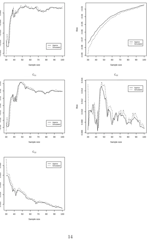
Figure 1 below plots the Monte Carlo simulated 2SLS bias and theO(T−1) approximate bias for a number of sample sizes. The two are very close, and it is clear that 2SLS estimation of the endogenous variable coefficient β1 is

not monotonically non increasing in the sample size, something that would be the case for estimation of a static model.

Figure 1: Approximate vs Simulated Bias in 2SLS estimation 30 40 50 60 70 80 90 100 −0.020 −0.015 −0.010 −0.005 0.000 Sample size Bias β1 Approx Simulated 30 40 50 60 70 80 90 100 −0.09 −0.08 −0.07 −0.06 −0.05 −0.04 −0.03 Sample size Bias λ Approx Simulated 30 40 50 60 70 80 90 100 −0.03 −0.02 −0.01 0.00 0.01 0.02 0.03 Sample size Bias C11 Approx Simulated 30 40 50 60 70 80 90 100 0.006 0.008 0.010 0.012 0.014 0.016 Sample size Bias C12 Approx Simulated 30 40 50 60 70 80 90 100 0.010 0.015 0.020 0.025 0.030 Sample size Bias C13 Approx Simulated

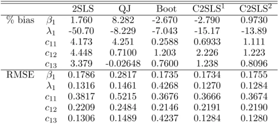
Table 1 presents empirical % bias and RMSE values for the parame-terisation above at a sample size of T = 50. The studies by Hsu, Lau, Fung, & Ulveling (1986) on static models and Ip (1991) on both static and dynamic models, cited earlier, used 200 and 500 Monte Carlo replications respectively when providing evidence for the 2SLS bootstrap bias correction. The number of bootstrap replicates considered were 150 and 300 by Hsu, Lau, Fung, & Ulveling (1986), and 200 by Ip (1991). It was found in our own simulation experiments that a relatively large number of replications were required, especially in cases with moderate or large 2SLS bias, and for the parameterisations and exogenous data that are considered. 100,000 or more Monte Carlo replications are used throughout when computing bias and mean squared error values in this section, which enables an accurate comparison of the three bias correction methods. 199 bootstrap replicates were used when obtaining the bias-corrected bootstrap. It can be seen from Table 1 that the 2SLS bias varies substantially across the parameters, with relatively small biases of around 3.4-4.4% for the exogenous variable coeffi-cientsc11, c12 and c13, 1.8% for the endogenous variable coefficient β1, and

51% for the lagged endogenous variable coefficientλ1.

Both C2SLS(1) and C2SLS(2) do well in terms of bias reduction for the model considered here, though C2SLS(2) is the only method that managed to reduce the bias for every coefficient. C2SLS(1) and C2SLS(2) also have reduced values for the empirical RMSE, though with L = 2 the estimator C2SLS(2) will not have a second moment, as mentioned earlier. We report the the empirical RMSE values anyway, as in Hahn, Hausman & Kuersteiner (2004) for the LIML estimator under the conventional normalisation where LIML does not have finite sample moments. It is worth noting that LIML does have finite sample moments under an alternative normalisation, though, as shown in Anderson (2010). See also Fuller (1977). Though the bootstrap has inflated RMSE values for estimation of λ1 and c13 in Model 1, this is

not observed in the other models that follow, except to a much lesser extent in Model 5, where there is a slight increase in RMSE for each parameter. The Quenouille Jackknife has inflated RMSE throughout, as was the case in Orcutt and Winokur (1969) and Liu-Evans and Phillips (2012) for estimation of autoregressive models.

Table 1. Model 1 % bias and RMSE, T = 50 2SLS QJ Boot C2SLS1 C2SLS2 % bias β1 1.760 8.282 -2.670 -2.790 0.9730 λ1 -50.70 -8.229 -7.043 -15.17 -13.89 c11 4.173 4.251 0.2588 0.6933 1.111 c12 4.448 0.7100 1.203 2.226 1.223 c13 3.379 -0.02648 0.7600 1.238 0.8096 RMSE β1 0.1786 0.2817 0.1735 0.1734 0.1755 λ1 0.1316 0.1461 0.4268 0.1270 0.1284 c11 0.3817 0.5215 0.3676 0.3666 0.3674 c12 0.2209 0.2484 0.2146 0.2191 0.2190 c13 0.1306 0.1489 0.4237 0.1284 0.1280

The original 2SLS bias in estimation ofβ1 is small in Model 1, and this

could make bias correction for it difficult, particularly given the much larger bias in estimation of λ1; it may also explain the inflated RMSE values for

the bootstrap. Model 2 below, and Models 3-5 in the next subsection, have original 2SLS biases of around 10-20% in absolute terms. Similar compar-isons are made between the various bias correction methods. The Model 2 coefficient matrices are

B = 1 −0.31 −β1 1 , Λ = −λ1 0 0 0 , and C= −c11 −c12 0 0 0 −c13 −0.31 0 −0.47 −0.16 −0.20 0 0 ,

where β1 = −0.43, c11 = 0.44, c12 = 0.40, c13 = 0.05 and λ1 = 0.59. The

maximum eigenvalue of Γ isτ = 0.52.

Table 2. Model 2 % bias and RMSE, T = 50

2SLS QJ Boot C2SLS1 C2SLS2 % bias β1 15.23 -9.081 -1.698 4.544 6.234 λ1 -13.31 -4.683 -3.324 -5.659 -5.180 c11 11.91 -2.178 1.5165 4.305 4.495 c12 9.687 3.371 -0.2232 3.224 3.895 c13 14.27 -15.40 1.002 4.538 4.833 RMSE β1 0.2901 0.5753 0.2740 0.2796 0.2710 λ1 0.1471 0.1964 0.1297 0.1287 0.1274 c11 0.4085 0.6465 0.3725 0.3789 0.3764 c12 0.2532 0.2966 0.2363 0.2451 0.2415 c13 0.1262 0.1603 0.1214 0.1219 0.1216

The bootsrap does particularly well here, and is the least biased in every case while also reducing the 2SLS RMSE. The Quenouille Jackknife and C2SLS methods reduce the bias, except the Quenouille Jackknife in one case.

3.2. Estimation with L=4

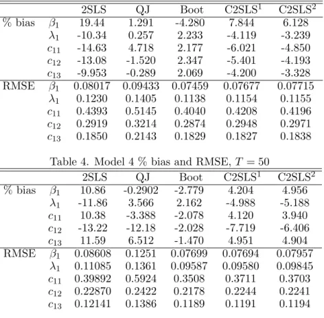
A further three models are considered, Models 3, 4, and 5, where L= 4 for the equation being estimated. An additional two exogenous variables are added to Equation 2, so that X = x1, x2, . . . , x8. The estimator C2SLS(2)

does not have a second moment here still, as the order of overidentification is onlyL= 2 for the second structural equation. The coefficient matrices in our simulations are as follows:

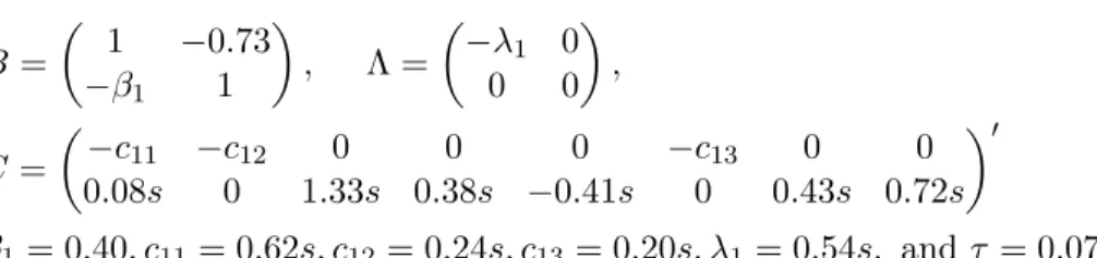
Model 3 B = 1 −1.44 −β1 1 , Λ = −λ1 0 0 0 , C = −c11 −c12 0 0 0 −c13 0 0 −0.11 0 −0.38 −1.08 0.82 0 −1.31 0.67 0 β1= 0.2, c11= 0.85, c12= 0.68, c13= 0.67, λ1 = 0.63, and τ = 0.88 Model 4 B = 1 −0.73 −β1 1 , Λ = −λ1 0 0 0 , C = −c11 −c12 0 0 0 −c13 0 0 0.08 0 1.33 0.38 −0.41 0 0.43 0.72 0 β1= 0.40, c11= 0.62, c12= 0.24, c13= 0.20, λ1= 0.54, and τ = 0.76 Model 5 B= 1 −1.19 −β1 1 , Λ = −λ1 0 0 0 , C= −c11 −c12 0 0 0 −c13 0 0 1.23 0 −0.08 −0.35 1.22 0 −0.38 −0.20 0 β1 = 0.43, c11=−0.76, c12=−1.47, c13= 0.78, λ1 = 0.38, and τ = 0.78

Estimation by Quenouille Jackknife is practically unbiased in some cases, for example the bias is just 0.257% in estimation of λ1 in Model 3, and there

are even smaller remaining biases for Model 5. In estimation ofc12 and c13

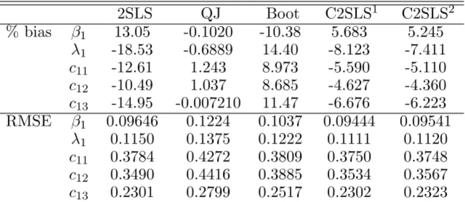
in Model 4, though, it does not reduce the bias as much as the bootstrap and C2SLS methods. Moreover, the RMSE is inflated in every case. The bootstrap performs well across Models 3 and 4, with both reduced bias and RMSE in estimation of each parameter. The C2SLS methods also reduce the bias, but not by as much, and the RMSE is marginally higher overall than with the bootstrap. Model 5 tells a different story, with the bootstrap reducing bias but not by as much as C2SLS, and with the RMSE slightly inflated when compared with 2SLS and C2SLS.

Table 3. Model 3 % bias and RMSE, T = 50

2SLS QJ Boot C2SLS1 C2SLS2 % bias β1 19.44 1.291 -4.280 7.844 6.128 λ1 -10.34 0.257 2.233 -4.119 -3.239 c11 -14.63 4.718 2.177 -6.021 -4.850 c12 -13.08 -1.520 2.347 -5.401 -4.193 c13 -9.953 -0.289 2.069 -4.200 -3.328 RMSE β1 0.08017 0.09433 0.07459 0.07677 0.07715 λ1 0.1230 0.1405 0.1138 0.1154 0.1155 c11 0.4393 0.5145 0.4040 0.4208 0.4196 c12 0.2919 0.3214 0.2874 0.2948 0.2971 c13 0.1850 0.2143 0.1829 0.1827 0.1838

Table 4. Model 4 % bias and RMSE, T = 50

2SLS QJ Boot C2SLS1 C2SLS2 % bias β1 10.86 -0.2902 -2.779 4.204 4.956 λ1 -11.86 3.566 2.162 -4.988 -5.188 c11 10.38 -3.388 -2.078 4.120 3.940 c12 -13.22 -12.18 -2.028 -7.719 -6.406 c13 11.59 6.512 -1.470 4.951 4.904 RMSE β1 0.08608 0.1251 0.07699 0.07694 0.07957 λ1 0.11085 0.1361 0.09587 0.09580 0.09845 c11 0.39892 0.5924 0.3508 0.3711 0.3703 c12 0.22870 0.2422 0.2178 0.2244 0.2241 c13 0.12141 0.1386 0.1189 0.1191 0.1194

Table 5. Model 5 % bias and RMSE, T = 50 2SLS QJ Boot C2SLS1 C2SLS2 % bias β1 13.05 -0.1020 -10.38 5.683 5.245 λ1 -18.53 -0.6889 14.40 -8.123 -7.411 c11 -12.61 1.243 8.973 -5.590 -5.110 c12 -10.49 1.037 8.685 -4.627 -4.360 c13 -14.95 -0.007210 11.47 -6.676 -6.223 RMSE β1 0.09646 0.1224 0.1037 0.09444 0.09541 λ1 0.1150 0.1375 0.1222 0.1111 0.1120 c11 0.3784 0.4272 0.3809 0.3750 0.3748 c12 0.3490 0.4416 0.3885 0.3534 0.3567 c13 0.2301 0.2799 0.2517 0.2302 0.2323

It seems clear that the C2SLS methods are competitive with the boot-strap and jackknife. The C2SLS1 estimator reduces bias in all but one case,

β1in Model 1, where the bootstrap and jackknife corrections also don’t seem

to work. The C2SLS2 estimator has a reduced bias in every case, perhaps due to its use of overidentifying information. The RMSE of the C2SLS1 esti-mator compares well with 2SLS in every case in our experiments. Moreover, no substantial improvement in bias reduction has been observed from using C2SLS(2) over C2SLS(1), indeed sometimes it is worse. While the success of C2SLS(1)may depend on the correct specification of the reduced form forY2,

the potential for mispecification to reduce the bias correction performance also seems greater in the case of C2SLS(2), where each structural equation needs to be estimated. The stronger requirement of having all equations overidentified, and to a higher order, makes it unlikely that an investigator would prefer C2SLS(2) over C2SLS(1), and it is therefore not investigated further.

3.3. Estimation with weak instruments

When instrumental variables are weak, it is well known that the perfor-mance of 2SLS can be very poor. Moreover, it has been shown by Hahn & Hausman (2002), Hahn, Hausman & Kuersteiner (2004) for a static model that the performance of 2SLS moment approximations can also be poor. Moreira, Porter, & Suarez (2004) provide examples where the bootstrap and higher order Edgeworth expansion are valid in weak instrument cases, but it is still unknown how the bootstrap will work in the present context of bias correction for 2SLS in dynamic models. Moreover, while the standard delete-1 jackknife method appears to work well in weak instruments cases in static models, see Hahn & Hausman (2002), Hahn, Hausman & Kuersteiner

(2004), it is unknown how the Quenouille Jackknife, chosen for its potential performance in dynamic models, will fare when there are weak instruments. All three bias correction methods performed quite well for Model 4 in terms of bias correction, particularly the bootstrap and Quenouille Jack-knife. Estimation by the bootstrap and C2SLS also resulted in a RMSE reduction. In order to consider cases with weaker instruments, new models are formed starting from Model 4 by shrinking the reduced form coeffi-cients towards zero while keeping the endogenous variable coefficoeffi-cients and the structural covariance matrix unchanged inBand Σ, respectively. Multi-plying Γ and Π by a constants∈(0,1) while holdingB fixed is equivalent to multplying Λ andCbys. As a measure of instrument weakness the expected

R2 from the first stage regression is used, namelyρ2= 1−_E[y0₂M y2/y20N y2]

where M =I−Z(Z0Z)Z0,N =I− _n1ιι0, and where ι is a T ×1 vector of ones.

Figure 2 below plots the bias approximation in Theorem 1 and the simu-lulated bias for the different ρ2 values achieved by using different values of

s. Smaller values of ρcorrespond to smaller values ofs; a value ofρ2= 0.20 was achieved using s = 0.1. Over the interval of ρ2 values that have been used in the figure, the bias approximation seems to do quite well in terms of its closeness to the true bias. It is also suggested by the figures that the bias approximation begins to break down as ρ2 is moved below 0.2 or, equivalently, as s is reduced below 0.1, and this is indeed the case. For sufficiently small values ofs, the true bias can be in the thousands, and the approximate bias is severely overstated.

Table 4 presents bias and RMSE values for 2SLS, QJ, bootstrap and C2SLS estimation of the following model where s= 0.1:

Model 4* B = 1 −0.73 −β1 1 , Λ = −λ1 0 0 0 , C= −c11 −c12 0 0 0 −c13 0 0 0.08s 0 1.33s 0.38s −0.41s 0 0.43s 0.72s 0 β1 = 0.40, c11= 0.62s, c12= 0.24s, c13= 0.20s, λ1 = 0.54s, andτ = 0.076

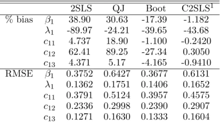
Model 4* is a case with weaker instruments where the bias approximation still appears to work, and this is reflected in the results for bias correction, which strongly favour C2SLS over the other methods. The bootstrap also

Figure 2: Approximate vs Simulated Bias given varying levels of instrument quality 0.2 0.4 0.6 0.8 1.0 20 40 60 80 100 E(R2₎ P ercentage Bias β1 Approx Simulated 0.2 0.4 0.6 0.8 1.0 −200 −150 −100 −50 E(R2₎ P ercentage Bias λ1 Approx Simulated 0.2 0.4 0.6 0.8 1.0 6 8 10 12 E(R2₎ P ercentage Bias C11 Approx Simulated 0.2 0.4 0.6 0.8 1.0 0 50 100 150 E(R2₎ P ercentage Bias C12 Approx Simulated 0.2 0.4 0.6 0.8 1.0 6 8 10 12 E(R2₎ P ercentage Bias C13 Approx Simulated

corrects the bias in this case to some degree, but does not perform nearly as well as C2SLS. The QJ corrects the bias in estimation of two out of five coefficients, and substantially increases the bias in two cases. All three methods inflate the RMSE, though for the bootstrap this increase in RMSE is not substantial.

Table 6. Model 4* % bias and RMSE, T = 50 2SLS QJ Boot C2SLS1 % bias β1 38.90 30.63 -17.39 -1.182 λ1 -89.97 -24.21 -39.65 -43.68 c11 4.737 18.90 -1.100 -0.2420 c12 62.41 89.25 -27.34 0.3050 c13 4.371 5.17 -4.165 -0.9410 RMSE β1 0.3752 0.6427 0.3677 0.6131 λ1 0.1362 0.1751 0.1406 0.1652 c11 0.3791 0.5124 0.3957 0.4575 c12 0.2336 0.2998 0.2390 0.2907 c13 0.1271 0.1630 0.1333 0.1604

Though the main objective of this section has been to investigate the ability to use the result in Theorem 1 for bias correction, and to compare this with other approaches, it may also be interesting to see how the densities and confidence sets for 2SLS and C2SLS compare in cases where the instruments are strong verses cases where the instruments are relatively weak. Figure 3 depicts the estimated densities and 95% confidence sets for 2SLS and C2SLS estimation of the Model 4 equation 1 structural coefficients. A Gaussian kernel with bandwidth parameter 0.5 was used throughout, and a lower number of Monte Carlo replications, 10000, was sufficient. It can be seen that the confidence sets are marginally larger for C2SLS in the case of β1

and λ, and marginally smaller for c11,c12 and c13.

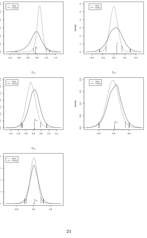
Figure 4 does the same for 2SLS and C2SLS estimation of Model 4* coefficients, and the picture changes somewhat. As in Figure 3, the location of the distribution appears substantially better in the case of C2SLS, though the spread is worse. There does not appear to be a clear winner between the bootstrap and C2SLS based on the results in Models 1-5 and 4*, though it may be concluded that both perform well overall, while the Quenouille jackknife fares less well.

Figure 3: C2SLS vs 2SLS densities, Model 4 (ρ2 = 0.92) 0.2 0.3 0.4 0.5 0.6 0.7 0.8 0 1 2 3 4 5 6 density β1 2SLS C2SLS β1 0.0 0.2 0.4 0.6 0.8 0 1 2 3 4 5 density λ1 2SLS C2SLS λ −1 0 1 2 0.0 0.2 0.4 0.6 0.8 1.0 1.2 density C11 2SLS C2SLS C11 −0.5 0.0 0.5 1.0 0.0 0.5 1.0 1.5 2.0 density C12 2SLS C2SLS C12 −0.2 0.0 0.2 0.4 0.6 0 1 2 3 4 density C13 2SLS C2SLS C13

Figure 4: C2SLS vs 2SLS densities, Model 4* (ρ2= 0.20) −1.0 −0.5 0.0 0.5 1.0 1.5 0.0 0.5 1.0 1.5 2.0 2.5 3.0 density β1 2SLS C2SLS β1 −0.4 −0.2 0.0 0.2 0.4 0 1 2 3 4 5 6 density λ1 2SLS C2SLS λ −1.5 −1.0 −0.5 0.0 0.5 1.0 1.5 0.0 0.2 0.4 0.6 0.8 1.0 1.2 1.4 density C11 2SLS C2SLS C11 −0.5 0.0 0.5 0.0 0.5 1.0 1.5 2.0 density C12 2SLS C2SLS C12 −0.5 0.0 0.5 0 1 2 3 4 density C13 2SLS C2SLS C13

4. Conclusion

The O(T−1) bias approximation for 2SLS in Nagar (1959) is one of the best known approximations in Econometrics and it has led not only to a better understanding of simultaneous equation bias in static models but has also provided a means of overcoming the problem through the development of bias corrected estimators; however it is invalid when the model includes lagged dependent endogenous variables anywhere in the system which is clearly a significant limitation. There has been some earlier work noted, based on the small-σ expansion, which has the attraction of relative sim-plicity, but it is well known that such an approach does not often work well in dynamic models; in particular the approximations may be less accurate than those provided by the more complex large-T expansion. It has now proved possible to extend the Nagar approximation to the dynamic case based on the large-T approach which represents a significant advance. The bias has two distinct parts; a part due to simultaneity and a part which derives from the dynamics of the equation. While the bias expression is long primarily due to the dynamic part, it has proved possible to use the approximation for practical bias reduction and the resulting bias corrected estimator is competitive with both the bootstrap and the Quenouille jack-knife on a bias criterion. In addition it was found to be better overall in terms of RMSE, as there is no inflation of the 2SLS RMSE. An example has also been presented where the bias in an endogenous variable coefficient does not appear to be monotonic in the sample size, suggesting that the result in Owen (1976) for static models does not go through for dynamic models.

The asymptotic approximation provided here has been obtained under a Normality assumption and has used a Nagar expansion methodology. The methodology in Phillips (2000) for 2SLS estimation of static models, or Bao and Ullah (2007), see also Rilstone, Srivastava and Ullah (1996), for GMM estimation of dynamic models, could potentially be used to extend the work here to non Normal settings; the validity assumptions for these approaches, stated in terms of smoothness conditions and the moments of model errors, are also perhaps more acceptable than for the Nagar method.

Appendix A

Calculating E[Q?R¯0u¯1]

It is clear thatE[Q?_R¯0_u¯ 1] = 0

Calculating E[Q?∆0₁u¯1]

It is clear thatE[Q?∆0₁u¯1] = 0 sinceE[W0L0u¯1] = 0

Calculating E[Q?∆0₂u¯1] E[Q?∆0₂u¯1] =Q?E[∆02u¯1]. Note that Q?∆0₂u¯1=Q?{Z¯(Z0Z)−1Z0[ ¯V2 : 0 : 0] + [LW I¯ ? 0 2 (Z 0 Z)−1Z0V¯2 : 0 : 0]}0u¯1 =Q?{[ ¯V2: 0 : 0]0Z(Z0Z)−1Z¯0+ [ ¯V2: 0 : 0]0Z(Z0Z)−1I2?W¯0L0}0u¯1 ={I₁?0V¯0Z¯(E[Z0Z])−1Z¯0+I₁?0V¯0Z¯(E[Z0Z])−1I₂?W¯0L0}u¯1 +Q?I₁?0V¯0W¯?(E[Z0Z])−1Z¯0u¯1 +op(T−1), since _ˆ Γ2−Γ2 ˆ Π2−Π2 = (Z0Z)−1Z0V¯2 = (E[Z0Z])−1Z¯0V¯2+ (E[Z0Z])−1W¯? 0 ¯ V2+op(T−1/2). This gives E[Q?∆0₂u¯1] =Q?I? 0 1 E[ ¯V 0_¯ Z(E[Z0Z])−1Z¯0u¯1]

(since the expectation of the last two terms is zero) =Q?I₁?0E[(S+ ¯u1φ0)0Z¯(E[Z0Z])−1Z¯0u] =Q?(tr{Z¯(E[Z0Z])−1Z¯0I₁?0}.I)(σ2φ). Calculating -E[Q?S1Q?R¯0u¯1] To order o(T−1), −E[Q?S1Q?R¯0u¯1] =−E[Q?{( ¯R0∆1+ ∆01R¯) + ( ¯R 0_∆ 2+ ∆02R¯) + (∆ 0 1∆1+ ∆02∆1) + (∆0₁∆1−E[∆01∆1])}Q?R¯0u¯1]

This leads to −E[Q?S1Q?R¯0u¯1] = −E[Q?( ¯R0LW A¯ +A0W¯0L0R¯)Q?R¯0u¯1] −E[Q?R¯0[LY¯( ˆΓ2−Γ2) +X( ˆΠ2−Π2) +LW¯( ˆΓ2−Γ2) : 0 : 0]Q?R¯0u¯1] −E[Q?[LY¯( ˆΓ2−Γ2) +X( ˆΠ2−Π2) +LW¯( ˆΓ2−Γ2) : 0 : 0]0RQ¯ ?R¯0u¯1] −E[Q?[LW¯Γ2 :LW¯1: 0]0[LY¯( ˆΓ2−Γ2) +X( ˆΠ2−Π2) +LW¯( ˆΓ2−Γ2) : 0 : 0]Q?R¯0u¯1] −E[Q?[LY¯( ˆΓ2−Γ2) +X( ˆΠ2−Π2) +LW¯( ˆΓ2−Γ2) : 0 : 0]0[LW¯Γ2 :LW¯1: 0]Q?R¯0u¯1] Using _ˆ Γ2−Γ2 ˆ Π2−Π2 = (Z0Z)−1Z0V¯2 = (E[Z0Z])−1Z¯0V¯2+ (E[Z0Z])−1W¯? 0 ¯ V2+op(T−1/2) and ˆ Γ2−Γ2 =I? 0 2 {(E[Z 0 Z])−1Z¯0V¯2+ (E[Z0Z])−1W¯? 0 ¯ V2}+op(T−1/2)

the non-zero terms become

−E[Q?R¯0LW AQ¯ ?R¯0u¯1]−E[Q?A0W¯0L0RQ¯ ?R¯0u¯1] −E[Q?R¯0Z¯(E[Z0Z])−1Z¯0V I¯ ₁?Q?R¯0u¯1]−E[Q?R¯0LW I¯ ? 0 2 (E[Z0Z])−1W¯? 0 ¯ V I₁?Q?R¯0u¯1] −E[Q?I₁?0V¯0Z¯(E[Z0Z])−1Z¯0RQ¯ ?R¯0u¯1]−E[Q?I? 0 1 V¯0W¯?(E[Z0Z])−1I2?W¯0L0RQ¯ ?R¯0u¯1] −E[Q?[LW¯Γ2 :LW¯1 : 0]0Z¯(E[Z0Z])−1W¯? 0 ¯ V I₁?Q?R¯0u¯1 −E[Q?I₁?0V¯0W¯?(E[Z0Z])−1Z¯0LW AQ¯ ?R¯0u¯1].

These are calculated in (a)-(i) below. For these calculations it is noted that

¯ W = T−1 X t=0 DtV¯Γt and LW¯ = T−1 X t=1 DtV¯Γt−1, where ¯V =S+ ¯u1φ0.

(a) −E[Q?R¯0LW AQ¯ ?R¯0u¯1] =−E[Q?R¯0 T−1 X t=1 DtV¯Γt−1AQ?R¯0u¯1] −E[Q?R¯0 T−1 X t=1 Dtu¯1φ0Γt−1AQ?R¯0u¯1] =−E[Q?R¯0 T−1 X t=1 Dtu¯1u¯01RQ¯ ?A0(Γt−1)0φ] −Q?R¯0 T−1 X t=1 DtRQ¯ ?A0(Γt−1)0(σ2φ) (b) −E[Q?A0W¯0L0RQ¯ ?R¯0u¯1] =−E[Q?A0 T−1 X t=1 Γt−10V¯0(Dt0RQ¯ ?R¯0u¯1] =−E[Q?A0 T−1 X t=1 Γt−10φu¯0₁Dt0] ¯RQ?R¯0u¯1 =−σ2Q?A0 T−1 X t=1 Γt−10φtr{R¯0Dt0RQ¯ ?} =−σ2Q?A0 T−1 X t=1 Γt−10φtr{R¯0Dt0RQ¯ ?} =−Q?A0 T−1 X t=1 Γt−10(tr{R¯0DtRQ¯ ?}.I)(σ2φ) (c) −E[Q?R¯0Z¯(E[Z0Z])−1Z¯0V I¯ ₁?Q?R¯0u¯1] =−E[Q?R¯0Z¯(E[Z0Z])−1Z¯0u¯1φ0I1?Q?R¯ 0 ¯ u1] =−Q?R¯0Z¯(E[Z0Z])−1Z¯0RQ¯ ?I₁?0(σ2φ) (d) −E[Q?R¯0LW I¯ ₂?0(E[Z0Z])−1W¯?0V I¯ ₁?Q?R¯0u¯1] = −E[Q?R¯0 T−1 X t=1 DtV¯Γt−1I₂?0(E[Z0Z])−1× PT−1 r=1 Γr −10 ¯ V0Dr0 0 ¯ V I₁?Q?R¯0u¯1]

In the final section of this Appendix, it is shown inNote 1that E[ ¯VΓt−1I₂?0(E[Z0Z])−1 PT−1 r=1 Γr−1 0_¯ V0Dr0 0 ¯ V I₁?Q?R¯0u¯1] =σ2Dr0RQ¯ ?I₁?0φtr{Ω[Γr−1 : 0](E[Z0Z])−1I₂?Γt−10} +σ2DrRQ¯ ?I₁?0ΩΓt−1I₂?0(E[Z0Z])−1I₂?Γr−10φ,

and therefore the final expression for (d) is

−Q?R¯0 T−1 X t,r=1 DtDr0RQ¯ ?(tr{Ω[Γr−1: 0](E[Z0Z])−1I₂?Γt−10}.I)I₁?0(σ2φ) −Q?R¯0 T−1 X t,r=1 DtDrRQ¯ ?I₁?0ΩΓt−1I₂?0(E[Z0Z])−1I₂?Γr−10(σ2φ), (e) −E[Q?I₁?0V¯0Z¯(E[Z0Z])−1Z¯0RQ¯ ?R¯0u¯1] =−E[Q?I? 0 1 φu¯01Z¯(E[Z0Z])−1Z¯0RQ¯ ?R¯0u¯1] =−Q?I₁?0φσ2tr{Z¯(E[Z0Z])−1Z¯RQ¯ ?R¯0} =−Q?(tr{Z¯(E[Z0Z])−1Z¯0RQ¯ ?R¯0}.I)I₁?0(σ2φ), (f ) −E[Q?I₁?0V¯0W¯?0(E[Z0Z])−1I₂?W¯0L0RQ¯ ?R¯0u¯1] =−E[Q?I₁?0V¯0( T−1 X t=1 DtV¯Γt−1: 0)(E[Z0Z])−1I₂?W¯0L0RQ¯ ?R¯0u¯1] =−E[Q?I₁?0V¯0( T−1 X t=1 DtV¯Γt−1: 0)(E[Z0Z])−1I₂? T−1 X r=1 Γr−10V¯0Dr0RQ¯ ?R¯0u¯1].

In in the final section of this Appendix, it is shown inNote 2that

E[ ¯V0DtV¯Γt−1I₂?0(E[Z0Z])−1I₂?Γr−10V¯0Dr0RQ¯ ?R¯0u¯1]

=σ2tr{ΩΓt−1I₂?0(E[Z0Z])−1I₂?Γr−10}tr{DtDr0RQ¯ ?R¯0}φ

and therefore the final expression for (f) is −Q? T−1 X r,t=1 (tr{ΩΓt−1I₂?0(E[Z0Z])−1I₂?Γr−10}.I)(tr{DtDr0RQ¯ ?R¯0}.I)I₁?0(σ2φ) −Q?I₁?0 T−1 X r,t=1 ΩΓr−1I₂?0(E[Z0Z])−1I₂?Γt−10(tr{DtRQ¯ ?R0Dr}.I)(σ2φ) (g) −E[Q?A0W¯0L0Z¯(E[Z0Z])−1W¯?0V I¯ ₁?Q?R¯0u¯1] =−E[Q?A0 T1 X t=1 Γt−10V¯0Dt0Z¯(E[Z0Z])−1 PT−1 r=1 Γr−1 0_¯ V0Dr0 00 ¯ V I₁?Q?R¯0u¯1].

In in the final section of this Appendix, it is shown inNote 3that

¯ V0Dt0Z¯(E[Z0Z])−1 PT−1 r=1 Γr −10 ¯ V0Dr0 00 ¯ V I₁?Q?R¯0u¯1 = ΩΓr−1I₂?0(E[Z0Z])−1Z¯0DtDr0RQ¯ ?I₁?0(σ2φ) + ΩI₁?Q?R¯0Dr0Dt0Z¯(E[Z0Z])−1I₂?Γr−10(σ2φ) and therefore the final expression for (g) is

−Q?A0 T−1 X r,t=1 Γt−10ΩΓr−1I₂?0(E[Z0Z])−1Z¯0DtDr0RQ¯ ?I₁?0(σ2φ) −Q?A0 T−1 X r,t=1 Γt−10ΩI₁?Q?R¯0Dr0Dt0Z¯(E[Z0Z])−1I₂?Γr−10(σ2φ) (h) −E[Q?A0W¯0L0LW I¯ ₂?0(E[Z0Z])−1Z¯0V I¯ ₁?Q?R¯0u¯1] =−E[Q?A0 T−1 X t=1 Γt−10V¯0Dt0 T−1 X r=1 DrV¯Γr−10I₂?0(E[Z0Z])−1Z¯0V I¯ ₁?Q?R¯0u¯1]

In in the final section of this Appendix, it is shown inNote 4that ¯

V0Dt0DrV¯Γr−10I₂?0(E[Z0Z])−1Z¯0V I¯ ₁?Q?R¯0u¯1

= (tr{Dt0DrZ¯(E[Z0Z])−1I₂?Γr−10ΩI₁?Q?R¯0}.I)(σ2φ) + ΩΓr−1I₂?0(E[Z0Z])−1Z¯0RQ¯ ?(tr{Dt0Dr}.I)I₁?0σ2φ

and therefore the final expression for (h) is −Q?A0 T−1 X t,r=1 Γt−10(tr{Dt0DrZ¯(E[Z0Z])−1I₂?Γr−10ΩI₁?Q?R¯0}.I)(σ2φ) −Q?A0 T−1 X t,r=1 Γt−10ΩΓr−1I₂?0(E[Z0Z])−1Z¯0RQ¯ ?(tr{Dt0Dr}.I)I₁?0σ2φ −Q?A0 T−1 X t,r=1 Γt−10ΩI₁?Q?R¯0Dr0DtZ¯(E[Z0Z])−1I₂?Γr−10(σ2φ) (i) −E[Q?I₁?0V¯0W¯?(E[Z0Z])−1Z¯0LW AQ¯ ?R¯0u¯1] −E[Q?I₁?0V¯0( T−1 X t=1 DtV¯Γt−1: 0)(E[Z0Z])−1Z¯0 T−1 X r=1 DrV¯Γr−1AQ?R¯u¯1]

In in the final section of this Appendix, it is shown inNote 5that

E[ ¯V0(DtV¯Γt−1 : 0)(E[Z0Z])−1Z¯0DrV¯Γr−1AQ?R¯u¯1]

=−(tr{DtDr0Z¯(E[Z0Z])−1I₂?Γt−10ΩΓr−1AQ?R¯0}.I)(σ2φ)

−ΩΓr−1AQ?R¯0σ2Dt0Dr0Z¯(E[Z0Z0])−1I₂?Γt−10(σ2φ) and therefore the final expression for (i) is

− T−1 X r,t=1 Q?(tr{DtDr0Z¯(E[Z0Z])−1I₂?Γt−10ΩΓr−1AQ?R¯0}.I)I₁?0(σ2φ) − T−1 X r,t=1 Q?I₁?0ΩΓr−1AQ?R¯0σ2Dt0Dr0Z¯(E[Z0Z0])−1I₂?Γt−10(σ2φ) Calculating -E[Q?S1Q?R¯0u¯1] E[Q?S1Q?∆01u¯1] =−E[Q?R¯0Z¯(E[Z0Z])−1W¯? 0 ¯ V I₁?Q?A0W¯0L0u¯1] −E[Q?I₁?0V¯0W¯?(E[Z0Z])−1Z¯0RQ¯ ?A0W¯0L0u¯1] −E[Q?A0W¯0L0Z¯0(E[Z0Z])−1Z¯0V I¯ ₁?Q?A0W¯0L0u¯1] −E[Q?A0W¯0L0LW L¯ 0LW I¯ ₂?0(E[Z0Z])−1W¯?0V I¯ ₁?Q?A0W¯0L0u¯1] −E[Q?{A0W¯0L0LW A¯ −E[A0W¯0L0LW A¯ ]}Q?A0W¯0L0u¯1] −E[Q?I₁?0V¯0Z¯(E[Z0Z])−1Z¯0LW AQ?A0W¯0L0u¯1] −E[Q?I₁?0V¯0W¯?(E[Z0Z])−1I₂?W¯0L0LW AQ¯ ?A0W¯0L0u¯1]

These are calculated in (a’)-(g’) below. (a’) −E[Q?R¯0Z¯(E[Z0Z])−1W¯?0V I¯ ₁?Q?A0W¯0L0u¯1] =−E[Q?R¯0Z¯(E[Z0Z])−1 T−1 X t=1 Γt−10V¯0Dt0 00 ¯ V I₁?Q?A0 T−1 X r=1 Γr−10V¯0Dr0u¯1] =−E[Q?R¯0Z¯(E[Z0Z])−1 T−1 X t=1 Γt−10 00 ¯ V0Dt0V I¯ ₁?Q?A0 T−1 X r=1 Γr−10V¯0Dr0u¯1]

In the final section of this Appendix, it is shown inNote 6that

E[ ¯V0Dt0V I¯ ₁?Q?A0Γr−10V¯0Dr0u¯1] = (tr{Dt

0

Dr}.I)ΩΓr−1AQ?I₁?0(σ2φ)

and therefore the final expression for (a’) is

−Q?R¯0Z¯(E[Z0Z])−1 T−1 X r,t=1 I₂?Γt−10(tr{Dt0Dr}.I)ΩΓr−1AQ?I₁?0(σ2φ) (b’) −E[Q?I₁?0V¯0W¯?(E[Z0Z])−1Z¯0RQ¯ ?A0W¯0L0u¯1] =−E[Q?I₁?0V¯( T−1 X t=1 DtV¯Γt−1 : 0)(E[Z0Z])−1Z¯0RQ¯ ?A0 T−1 X r=1 Γr−10V¯0Dr0u¯1]

In in the final section of this Appendix, it is shown inNote 7that

E[ ¯V(DtV¯Γt−1 : 0)(E[Z0Z])−1Z¯0RQ¯ ?A0Γr−10V¯0Dr0u¯1]

=tr{DtDr0}(tr{ΩΓt−1I₂?0(E[Z0Z])−1Z¯0RQ¯ ?A0Γr−10}.I)(σ2φ)

and therefore the final expression for (b’) is

−Q? T1 X r,t=1 (tr{DtDr0}.I)(tr{ΩΓt−1I₂?0(E[Z0Z])−1Z¯0RQ¯ ?A0Γr−10}.I)I₁?0(σ2φ) (c’) −E[Q?A0W¯0L0Z¯(E[Z0Z])−1Z¯0V I¯ ₁?Q?A0W¯0L0u¯1] =−E[Q?A0 T−1 X t=1 Γt−10V¯0Dt0Z¯(E[Z0Z])−1Z¯0V I¯ ₁?Q?A0 T−1 X r=1 Γr−10V¯0Dr0u¯1].

In in the final section of this Appendix, it is shown inNote 8that E[ ¯V0Dt0Z¯(E[Z0Z])−1Z¯0V I¯ ₁?Q?A0 T−1 X r=1 Γr−10V¯0Dr0u¯1] =tr{ΩI₁?Q?A0Γr−10}(tr{Dt0Z¯(E[Z0Z])−1Z¯0Dr0}.I)(σ2φ) + (tr{Dt0Z¯(E[Z0Z])−1Z¯0Dr}.I)ΩΓr−1AQ?I₁?0(σ2φ)

and therefore the final expression for (c’) is

−Q?A0 T−1 X r,t=1 Γt−10(tr{ΩI₁?Q?A0Γr−10}.I)(tr{Dt0Z¯(E[Z0Z])−1Z¯0Dr0}.I)(σ2φ) (d’) −E[Q?A0W¯0L0LW I¯ ₂?0(E[Z0Z])−1W¯?0V I¯ ₁?Q?A0W¯0L0u¯1] =−E[Q?A0E[ ¯W0L0LW¯]I₂?0(E[Z0Z])−1W¯?0V I¯ ₁?Q?A0W¯0L0u¯1]

to order Op(T−1). Therefore, to order Op(T−1),

−E[Q?A0W¯0L0LW I¯ ₂?(E[Z0Z])−1W¯?0V I¯ ₁?Q?A0W¯0L0u¯1] =−E[Q?A0E[ ¯W0L0LW¯]I₂?0(E[Z0Z])−1 PT−1 t=1 Γt −10 ¯ V0Dt0 00 ¯ V I₁?Q?A0 T−1 X t−1 Γr−10V¯0Dr0u¯1]

In in the final section of this Appendix, it is shown inNote 9that

E[ ¯V0Dt0V I¯ ₁?Q?A0Γr−10V¯0Dr0u¯1] = ΩΓr−1AQ?(tr{Dt

0

Dr}.I)I₁?0(σ2φ)

and therefore the final expression for (d’) is

−Q?A0E[ ¯W0L0LW¯]I₂?0(E[Z0Z])−1 T−1 X r,t=1 I₂?Γt−10ΩΓr−1AQ?(tr{Dt0Dr}.I)I₁?0(σ2φ) (e’) −E[Q?A0W¯0L0LW AQ¯ ?A0W¯0L0u¯1] = −E[Q?A0 T−1 X r,t,s=1 Γt−10V¯0Dt0DrΓr−1AQ?A0Γs−10V¯0Ds0u¯1].

In in the final section of this Appendix, it is shown inNote 10 that

E[ ¯V0Dt0DrΓr−1AQ?A0Γs−10V¯0Ds0u¯1] =

ΩΓs−1AQ?A0Γr−10{tr(Dt0DrDs).I}(σ2φ) +tr(ΩΓr−1AQ?A0Γs−10)tr(Dt0DrDs0)(σ2φ),

and therefore the final expression for (e’) is

−Q? T−1 X r,t,s=1 A0Γt−10ΩΓs−1AQ?A0Γr−10{tr(Dt0DrDs).I}(σ2φ) −Q? T−1 X r,t,s=1 A0Γt−10tr(ΩΓr−1AQ?A0Γs−10)tr(Dt0DrDs0)(σ2φ) (f ’) −E[Q?I₁?0V¯0Z¯(E[Z0Z])−1Z¯0LW AQ¯ ?A0W¯0L0u¯1] =−E[Q?I₁?0V¯0Z¯(E[Z0Z])−1Z¯0 T−1 X r,t DtV¯Γt−1AQ?A0Γr−10V¯0Dr0u¯1].

In in the final section of this Appendix, it is shown inNote 11 that

E[ ¯V0Z¯(E[Z0Z])−1Z¯0DtV¯Γt−1AQ?A0Γr−10V¯0Dr0u¯1]

= (tr{ΩΓt−1AQ?A0Γr−10}.I)(tr{Z¯(E[Z0Z])−1Z¯0DtDr0}.I)(σ2φ) + ΩΓr−1AQ?A0Γt−10(tr{Z¯(E[Z0Z])−1Z¯0DtDr}.I)(σ2φ)

and therefore the final expression for (f’) is

− T−1 X r,t=1 Q?(tr{ΩΓt−1AQ?A0Γr−10}.I)(tr{Z¯(E[Z0Z])−1I₂?W¯0L0LW AQ¯ ?A0W¯0L0u¯1}.I)I? 0 1 (σ2φ) − T−1 X r,t=1 Q?I₁?0ΩΓr−1AQ?A0Γt−10(tr{Z¯(E[Z0Z])−1ZD¯ tDr}.I)(σ2φ) (g’) −E[Q?I₁?0V¯0W¯?(E[Z0Z])−1I₂?0W¯0L0LW AQ¯ ?A0W¯0L0u¯1] −E[Q?I₁?0V¯0W¯?(E[Z0Z])−1I₂?0E[ ¯W0L0LW¯]AQ?A0W¯0L0u¯1]

to order Op(T−1). Therefore, to order Op(T−1), −E[Q?I₁?0V¯0W¯?(E[Z0Z])−1I₂?0W¯0L0LW AQ¯ ?A0W¯0L0u¯1] =−E[Q?I₁?0V¯0( T−1 X t=1 DtV¯Γt−1 : 0)(E[Z0Z])−1I₂?0E[ ¯W0L0LW¯]AQ?A0 T−1 X r=1 Γr−10V¯0Dr0u¯1].

In in the final section of this Appendix, it is shown inNote 12 that

¯

V0(DtV¯Γt−1: 0)(E[Z0Z])−1I₂?0E[ ¯W0L0LW¯]AQ?A0Γr−10V¯0Dr0u¯1

=tr{Ω(Γt−1 : 0)(E[Z0Z])−1I₂?E[W0L0LW]AQ?A0Γr−10}(tr{DtDr0}.I)(σ2φ)

and therefore the final expression for (g’) is

−

?

X

r,t=1

Q?(tr{Ω(Γt−1: 0)(E[Z0Z])−1I₂?E[W0L0LW]AQ?A0Γr−10}(tr{DtDr0}.I)I₁?0(σ2φ)

Rearranging for the final expression

In the following all the expectations calculations for the terms in equation (23) are added together, in the order that they appear. Recall that QZ = (E[Z0Z])−1. Q?(tr{ZQ¯ ZZ¯0}.I)I? 0 1 (σ2φ) −Q?R¯0 T−1 X t=1 DtRQ¯ ?A0(Γt−1)0(σ2φ) −Q?A0 T−1 X t=1 Γt−10(tr{R¯0DtRQ¯ ?}.I)(σ2φ) −Q?R¯0ZQ¯ ZZ¯0RQ¯ ?I? 0 1 (σ2φ) −Q?R¯0 T−1 X t,r=1 DtDr0RQ¯ ?(tr{ΩΓr−1I₂?0QZI2?Γt −10 }.I)(σ2I₁?0φ) −Q?R¯0 T−1 X t,r=1 DtDrRQ¯ ?I₁?0ΩΓt−1I₂?0QZI2?Γr−1 0 (σ2φ) −Q?(tr{ZQ¯ ZZ¯0RQ¯ ?R¯0}.I)I? 0 1 (σ2φ) −Q? T−1 X r,t=1 (tr{ΩΓt−1I₂?0QZI2?Γr−1 0 }.I)(tr{DtDr0RQ¯ ?R¯0}.I)I₁?0(σ2φ)

−Q?I₁?0 T−1 X r,t=1 ΩΓr−1I₂?0QZI2?Γt −10 (tr{DtRQ¯ ?R0Dr}.I)(σ2φ) −Q?A0 T−1 X r,t=1 Γt−10ΩΓr−1I₂?0QZZ¯0DtDr 0 ¯ RQ?I₁?0(σ2φ) −Q?A0 T−1 X r,t=1 Γt−10ΩI₁?Q?R¯0Dr0Dt0ZQ¯ ZI2?Γr −10 (σ2φ) −Q?A0 T−1 X t,r=1 Γt−10(tr{Dt0DrZQ¯ ZI2?Γr −10 ΩI₁?Q?R¯0}.I)(σ2φ) −Q?A0 T−1 X t,r=1 Γt−10ΩΓr−1I₂?0QZZ¯0RQ¯ ?(tr{Dt 0 Dr}.I)I₁?0(σ2φ) −Q?A0 T−1 X t,r=1 Γt−10ΩI₁?Q?R¯0Dr0DtZQ¯ ZI2?Γr −10 (σ2φ) −Q? T−1 X t,r=1 (tr{DtDr0ZQ¯ ZI2?Γt−1 0 ΩΓr−1AQ?R¯0}.I)I₁?0(σ2φ) −Q? T−1 X t,r=1 I₁?0ΩΓr−1AQ?R¯0σ2Dt0Dr0ZQ¯ ZI2?Γt−1 0 (σ2φ) −Q?R¯0ZQ¯ Z T−1 X r,t=1 I₂?Γt−10(tr{Dt0Dr}.I)ΩΓr−1AQ?I₁?0(σ2φ) −Q? T−1 X r,t=1 (tr{DtDr0}.I)(tr{ΩΓt−1I₂?0QZZ¯0RQ¯ ?A0Γr−1 0 }.I)I₁?0(σ2φ) −Q?A0 T−1 X r,t=1 Γt−10(tr{ΩI₁?Q?A0Γr−10}tr{Dt0ZQ¯ ZZ¯0Dr 0 }.I)(σ2φ) −Q?A0 T−1 X r,t=1 Γt−10(tr{Dt0ZQ¯ ZZ¯0Dr}.I)ΩΓr−1AQ?I? 0 1 (σ2φ) −Q?A0E[ ¯W0L0LW¯]I₂?0QZ T−1 X r,t=1 I₂?Γt−10ΩΓr−1AQ?(tr{Dt0Dr}.I)I₁?0(σ2φ)

−Q? T−1 X r,t,s=1 A0Γt−10ΩΓs−1AQ?A0Γr−10{tr(Dt0DrDs).I}(σ2φ) −Q? T−1 X r,t,s=1 A0Γt−10tr(ΩΓr−1AQ?A0Γs−10)tr(Dt0DrDs0)(σ2φ) −Q? T−1 X r,t=1 (tr{ΩΓt−1AQ?A0Γr−10}.I)(tr{ZQ¯ ZZ¯0DtDr 0 }.I)I₁?0(σ2φ) −Q?I₁?0 T−1 X r,t=1 ΩΓr−1AQ?A0Γt−10(tr{ZQ¯ ZZ¯0DtDr}.I)(σ2φ) − T−1 X r,t=1 Q?(tr{ΩΓt−1I₂?0QZI? 0 2 E[W0L0LW]AQ?A0Γr−1 0 }.I)(tr{DtDr0}.I)I₁?0(σ2φ)

Next recall thatϕ=σ2φ,ψ =I₁?0ϕ, (Γr−1 : 0) = Γr−1I₂?0,I₂?0QZI2? =Q?Z, and QW =

PT−1

t=1 (T −t)Γt −10

ΩΓt−1. Also, note that tr{Dt0Dr} = T −t

when t=r and 0 otherwise. The terms above can then be written (in the same order) as follows:

Q?(tr{ZQ¯ ZZ¯0}.I)ψ −Q?R¯0 T−1 X t=1 DtRQ¯ ?A0(Γt−1)0ϕ −Q?A0 T−1 X t=1 Γt−10(tr{R¯0DtRQ¯ ?}.I)ϕ −Q?R¯0ZQ¯ ZZ¯0RQ¯ ?ψ −Q?R¯0 T−1 X t,r=1 DtDr0RQ¯ ?(tr{ΩΓr−1Q?_ZΓt−10}.I)ψ −Q?R¯0 T−1 X t,r=1 DtDrRQ¯ ?I₁?0ΩΓt−1Q?_ZΓr−10ϕ −Q?(tr{ZQ¯ ZZ¯0RQ¯ ?R¯0}.I)ψ −Q? T−1 X r,t=1 (tr{Γr−10ΩΓt−1Q?_Z}.I)(tr{DtDr0RQ¯ ?R¯0}.I)ψ

−Q?I₁?0 T−1 X r,t=1 ΩΓr−1Q?_ZΓt−10(tr{DtRQ¯ ?R0Dr}.I)ϕ −Q?A0 T−1 X r,t=1 Γt−10ΩΓr−1I₂?0QZZ¯0DtDr 0 ¯ RQ?ψ −Q?A0 T−1 X r,t=1 Γt−10ΩI₁?Q?R¯0Dr0Dt0ZQ¯ ZI2?Γr −10 ϕ −Q?A0 T−1 X t,r=1 Γt−10(tr{Dt0DrZQ¯ ZI2?Γr −10 ΩI₁?Q?R¯0}.I)ϕ −Q?A0QWI? 0 2 QZZ¯0RQ¯ ?ψ −Q?A0 T−1 X t,r=1 Γt−10ΩI₁?Q?R¯0Dr0DtZQ¯ ZI2?Γr−1 0 ϕ −Q? T−1 X t,r=1 (tr{DtDr0ZQ¯ ZI2?Γt −10 ΩΓr−1AQ?R¯0}.I)ψ −Q? T−1 X t,r=1 I₁?0ΩΓr−1AQ?R¯0Dt0Dr0ZQ¯ ZI2?Γt −10 ϕ −Q?R¯0ZQ¯ ZI2?QWAQ?ψ −Q?(tr{QWI? 0 2 QZZ¯0RQ¯ ?A0}.I)ψ −Q?A0 T−1 X r,t=1 Γt−10(tr{ΩI₁?Q?A0Γr−10}tr{Dt0ZQ¯ ZZ¯0Dr 0 }.I)ϕ −Q?A0 T−1 X r,t=1 Γt−10(tr{Dt0ZQ¯ ZZ¯0Dr}.I)ΩΓr−1AQ?ψ −Q?A0QWQ?ZQWAQ?ψ −Q? T−1 X r,t,s=1 A0Γt−10ΩΓs−1AQ?A0Γr−10{tr(Dt0DrDs).I}ψ −Q? T−1 X r,t,s=1 A0Γt−10tr(ΩΓr−1AQ?A0Γs−10)tr(Dt0DrDs0)ψ

−Q? T−1 X r,t=1 (tr{ΩΓt−1AQ?A0Γr−10}.I)(tr{ZQ¯ ZZ¯0DtDr 0 }.I)ψ −Q?I₁?0 T−1 X r,t=1 ΩΓr−1AQ?A0Γt−10(tr{ZQ¯ ZZ¯0DtDr}.I)ϕ −Q?(tr{QWQZ?QWAQ?A0}.I)ψ

Appendix B

Note 1 E[ ¯VΓt−1I₂?0(E[Z0Z])−1 Γr−10_¯ V0Dr0 0 ¯ V I₁?Q?R¯0u¯1] =E[¯u1φ0Γt−1I? 0 2 (E[Z 0 Z])−1I₂?Γr−10φu¯0₁Dr0u¯1φ0I1?Q?R¯ 0 ¯ u1] (32) +E[SΓt−1I₂?0(E[Z0Z])−1I₂?Γr−10S0Dr0u¯1φ0I1?Q?R¯ 0 ¯ u1] (33) +E[¯u1φ0Γt−1I? 0 2 (E[Z0Z])−1I2?Γr−1 0 S0Dr0SI₁?Q?R¯0u¯1] (34) +E[SΓt−1I₂?0(E[Z0Z])−1I₂?Γr−10φu¯0₁Dr0SI₁?Q?R¯0u¯1] (35) (32) is calculated as follows: E[¯u1u¯01RQ¯ ? 0 I₁?0φφ0Γt−1I₂?0(E[Z0Z])−1I₂? Γr−10 0 φu¯0₁Dr0u¯1] =σ4{tr(Dr).I+Dr+Dr0}RQ¯ ?0I₁?0φφ0Γt−1I₂?0(E[Z0Z])−1I₂?Γr−10φ =σ4{Dr+Dr0}RQ¯ ?0I₁?0φφ0Γt−1I₂?0(E[Z0Z])−1I₂?Γr−10φ (33) is calculated as follows: E[SΓt−1I₂?0(E[Z0Z])−1 Γr−10 00 S0Dr0u¯1u¯ 0 1RQ¯ ? 0 I₁?0φ] = (tr{C₂?Γt−1I₂?0(E[Z0Z])−1I₂?Γr−10}Dr0σ2RQ¯ ?0I₁?0φ,

using SN S0 =tr(C₂?N).I from Lemma 1. (34) is calculated as follows: E[¯u1u¯01RQ¯ ? 0 I₁?0S0DrS Γr−10 0 0 (E[Z0Z])−1I₂?Γt−10φ] =σ2RQ¯ ?I₁?0E[S0DrS]Γr−1I₂?0(E[Z0Z])−1I₂?Γt−10φ =σ2RQ¯ ?I₁?0{tr(Dr)}C₂?Γr−1I₂?0(E[Z0Z])−1I₂?Γt−10φ

using E[S0N S] ={tr(N)}.C₂? from Lemma 1.

(35) can be written as follows, recalling thatS and ¯u1 are independent, and

recalling from Lemma 1 thatSN S =N0C?

2: E[SDru¯1φ0Γr−1I? 0 2 (E[Z 0 Z])−1I₂?Γt−10C₂?I₁?Q?R¯0u¯1].

Then E[SDru¯1φ0Γr−1I? 0 2 (E[Z0Z])−1I2?Γt−1 0 C₂?I₁?Q?R¯0u¯1] =E[Dru¯1u¯01RQ¯ ?I? 0 1 C2?Γt−1I? 0 2 (E[Z0Z])−1I2?Γr−1 0 φ] =σ2DrRQ¯ ?I₁?0C₂?Γt−1I₂?0(E[Z0Z])−1I₂?Γr−10φ =σ2DrRQ¯ ?I₁?0ΩΓt−1I₂?0(E[Z0Z])−1I₂?Γr−10φ −σ4DrRQ¯ ?I₁?0φφ0Γt−1I₂?0(E[Z0Z])−1I₂?Γr−10φ

Putting these together gives

E[ ¯VΓt−1I₂?0(E[Z0Z])−1 Γr−10V¯0Dr0 0 ¯ V I₁?Q?R¯0u¯1] =σ2Dr0RQ¯ ?I₁?0φtr{ΩΓr−1I₂?0(E[Z0Z])−1I₂?Γt−10} +σ2DrRQ¯ ?I₁?0ΩΓt−1I₂?0(E[Z0Z])−1I₂?Γr−10φ, Note 2 E[ ¯V0DtV¯Γt−1I₂?0(E[Z0Z])−1I₂?Γr−10V¯0Dr0RQ¯ ?R¯0u¯1] =E[φu¯0₁Dtu¯1φ0Γt−1I? 0 2 (E[Z0Z])−1I2?Γr−1 0 φu¯0₁Dr0RQ¯ ?R¯0u¯1] (36) +E[φu¯0₁DtSΓt−1I₂?0(E[Z0Z])−1I₂?Γr−10S0Dr0RQ¯ ?R¯0u¯1] (37) +E[S0Dtu¯1φ0Γt−1I? 0 2 (E[Z0Z])−1I2?Γr−1 0 S0Dr0RQ¯ ?R¯0u¯1] (38) +E[S0DtSΓt−1I₂?0(E[Z0Z])−1I₂?Γr−10φu¯0₁Dr0RQ¯ ?R¯0u¯1] (39) (36) becomes φφ0Γt−1I₂?0(E[Z0Z])−1P₂0Γr−10φtr{(Dt+Dt0)Dr0RQ¯ ?R¯0} (37) becomes σ2tr{ΩΓt−1I₂?0(E[Z0Z])−1I₂?Γr−10}tr{DtDr0RQ¯ ?R¯0}φ −σ4tr{φφ0Γt−1I₂?0(E[Z0Z])−1I₂?Γr−10}tr{DtDr0RQ¯ ?R¯0}φ (38) becomes σ2tr(DtrQ¯ ?R¯0Dr)ΩΓr−1I₂?0(E[Z0Z])−1I₂?Γt−10φ −σ4tr(DtrQ¯ ?R¯0Dr)φφ0Γr−1I₂?0(E[Z0Z])−1I₂?Γt−10φ

(39) becomes zero, and putting these together gives E[ ¯V0DtV¯Γt−1I₂?0(E[Z0Z])−1I₂?Γr−10V¯0Dr0RQ¯ ?R¯0u¯1] =σ2tr{ΩΓt−1I₂?0(E[Z0Z])−1I₂?Γr−10}tr{DtDr0RQ¯ ?R¯0}φ +σ2tr{DtRQ¯ ?R0Dr}ΩΓr−1I₂?0(E[Z0Z])−1I₂?Γt−10φ Note 3 E[ ¯V0Dt0Z¯(E[Z0Z])−1 Γr−10 00 ¯ V0Dr0V I¯ ₁?Q?R¯0u¯1] =E[φu¯0₁Dt0Z¯(E[Z0Z])−1I₂?Γr−10φu¯0₁Dr0u¯1φ0I1?Q?R¯0u¯1] (40) +E[φu¯0₁Dt0Z¯(E[Z0Z])−1I₂?Γr−10S0Dr0SI₁?Q?R¯0u¯1] (41) +E[S0Dt0Z¯(E[Z0Z])−1I₂?Γr−10S0Dr0u¯1φ0I1?Q?R¯0u¯1] (42) +E[S0Dt0Z¯(E[Z0Z])−1I₂?Γr−10φu¯0₁Dr0SI₁?Q?R¯0u¯1] (43) (40) becomes σ4φ0I₁?Q?R¯0DrDt0Z¯(E[Z0Z])−1I₂?Γr−10φφ0 +σ4φ0I₁?Q?R¯0Dr0DtZ¯(E[Z0Z])−1I₂?Γr−10φφ0 (41) is zero (42) becomes σ2ΩΓt−1I₂?0(E[Z0Z])−1Z0DtDr0RQ¯ ?I₁?0φ −σ4φφ0I₁?Q?R¯0DrDt0Z¯(EZ0Z)−1I₂?Γt−10φ (43) becomes σ2ΩI₁?Q?RD¯ r0Dt0Z¯(EZ0Z)−1I₂?Γr−10φ −σ4φφ0I₁?Q?RD¯ r0Dt0Z¯(EZ0Z)−1I₂?Γr−10φ. These reduce to E[ ¯V0Dt0Z¯(E[Z0Z])−1 PT−1 r=1 Γr −10 ¯ V0Dr0 00 ¯ V I₁?Q?R¯0u¯1] = ΩΓr−1I₂?0(E[Z0Z])−1Z¯0DtDr0RQ¯ ?I₁?0(σ2φ) + ΩI₁?Q?R¯0Dr0Dt0Z¯(E[Z0Z])−1I₂?Γr−10(σ2φ)

Note 4 E[ ¯V0Dt0DrV¯Γr−10I₂?0(E[Z0Z])−1Z¯0V I¯ ₁?Q?R¯0u¯1] =E[φu¯0₁Dt0Dru¯1φ0Γr−1 0 I₂?0(E[Z0Z])−1Z¯0u¯1φ0I1?Q?R¯ 0 ¯ u1] (44) +E[φu¯0₁Dt0DrSΓr−10I₂?0(E[Z0Z])−1Z¯0SI₁?Q?R¯0u¯1] (45) +E[S0Dt0DrSΓr−10I₂?0(E[Z0Z])−1Z¯0u¯1φ0I1?Q?R¯ 0 ¯ u1] (46) +E[S0Dt0Dru¯1φ0Γr−1 0 I₂?0(E[Z0Z])−1Z¯0SI₁?Q?R¯0u¯1] (47) (44) becomes σ4φtr[1 2{D t0_Dr_+Dr0_Dt_}]tr{RQ¯ ?_I?0 1 φφ 0_Γr−1_I?0 2 (E[Z 0_Z])−1_Z¯0_} + 2σ4φtr[1 2{D t0_Dr_+Dr0_Dt_}RQ¯ ?_I?0 1 φφ0Γr−1I? 0 2 (E[Z0Z])−1Z¯0] (45) becomes σ2φtr[Dt0DrZ¯(E[Z0Z])−1I₂?Γr−10ΩI₁?Q?R¯0] −σ4φtr[Dt0DrZ¯(E[Z0Z])−1I₂?Γr−10φφ0I₁?Q?R¯0] (46) becomes σ2tr{Dt0Dr}ΩΓr−1I₂?0(E[Z0Z])−1Z¯0RQ¯ ?I₁?0φ −σ4tr{Dt0Dr}φφ0Γr−1I₂?0(E[Z0Z])−1Z¯0RQ¯ ?I₁?0φ (47) becomes σ2ΩI₁?Q?R¯0Dr0DtZ¯(E[Z0Z])−1I₂?Γr−10φ −σ2φφ0Γr−1I₂?0(E[Z0Z])−1Z¯0Dt0DrRQ¯ ?I₁?φ

Putting these together gives

E[ ¯V0Dt0DrV¯Γr−10I₂?0(E[Z0Z])−1Z¯0V I¯ ₁?Q?R¯0u¯1]

= (tr{Dt0DrZ¯(E[Z0Z])−1I₂?Γr−10ΩI₁?Q?R¯0}.I)(σ2φ) + ΩΓr−1I₂?0(E[Z0Z])−1Z¯0RQ¯ ?(tr{Dt0Dr}.I)I₁?0σ2φ

Note 5 E[ ¯V0(DtV¯Γt−1 : 0)(E[Z0Z])−1Z¯0DrV¯Γr−1AQ?R¯u¯1] =E[φu¯0₁Dtu¯1φ0Γt−1I? 0 2 (E[Z0Z])−1Z¯0Dru¯1φ0Γr−1AQ?R¯u¯1] (48) +E[φu¯0₁DtSΓt−1I₂?0(E[Z0Z])−1Z¯0DrSΓr−1AQ?R¯u¯1] (49) +E[S0DtSΓt−1I₂?0(E[Z0Z])−1Z¯0Dru¯1φ0Γr−1AQ?R¯u¯1] (50) +E[S0Dtu¯1φ0Γt−1I2?(E[Z 0_Z])−1_Z¯0_Dr_SΓr−1_AQ?_R¯u¯ 1] (51) (48) becomes 2φσ4tr{1 2(D t_+Dr0 )Dr0Z¯(E[Z0Z])−1I₂?Γt−10φφ0Γr−1AQ?R¯0} (49) becomes σ2φtr{DtDr0Z¯(E[Z0Z])−1I₂?Γr−10ΩΓr−1AQ?R¯0} −σ4φtr{DtDr0Z¯(E[Z0Z])−1I₂?Γr−10φφ0Γr−1AQ?R¯0} (50) is zero (51) becomes σ2Ω{DtRQ¯ ?A0Γr−10}0Dr0Z¯(E[Z0Z])−1I₂?Γt−10φ −σ2φφ{DtRQ¯ ?A0Γr−10}0Dr0Z¯(E[Z0Z])−1I₂?Γt−10φ

using E[W0N0W0] =C₂?N (see Lemma 1). Putting these together gives

E[ ¯V0DtV¯Γt−1I₂?0(E[Z0Z])−1Z¯0DrV¯Γr−1AQ?R¯u¯1] =−(tr{DtDr0Z¯(E[Z0Z])−1I₂?Γt−10ΩΓr−1AQ?R¯0}.I)(σ2φ) −ΩΓr−1AQ?R¯0σ2Dt0Dr0Z¯(E[Z0Z0])−1I₂?Γt−10(σ2φ) Note 6 E[ ¯V0Dt0V I¯ ₁?Q?A0Γr−10V¯0Dr0u¯1] =E[φu¯0₁Dt0u¯1φ0I1?Q?A0Γr−1 0 φu¯0₁Dr0u¯1] (52) +E[φu¯0₁Dt0SI₁?Q?A0Γr−10S0Dr0u¯1] (53) +E[S0Dt0SI₁?Q?A0Γr−10φu¯0₁Dr0u¯1] (54)

+E[S0Dt0u¯1φ0I1?Q?A 0 Γr−10S0Dr0u¯1] (55) (52) becomes σ4φφ0I₁?Q?A0Γr−10φ[2tr{1 2(D t_+Dt0_)Dr0_}] (53) is zero (54) is zero (55) becomes σ2tr(Dt0Dr)ΩΓr−1AQ?I₁?0φ −σ4tr(Dt0Dr)φφ0Γr−1AQ?I₁?0φ

Putting these together gives

E[ ¯V0Dt0V I¯ ₁?Q?A0Γr−10V¯0Dr0u¯1] = (tr{Dt 0 Dr}.I)ΩΓr−1AQ?I₁?0(σ2φ) Note 7 E[ ¯V DtV¯Γt−1I₂?0(E[Z0Z])−1Z¯0RQ¯ ?A0Γr−10V¯0Dr0u¯1] =E[φu¯0₁Dtu¯1φ0Γt−1I? 0 2 (E[Z0Z])−1Z¯0RQ¯ ?A0Γr−1 0 φu¯0₁Dr0u¯1] (56) +E[φu¯0₁DtSΓt−1I₂?0(E[Z0Z])−1Z¯0RQ¯ ?A0Γr−10S0Dr0u¯1] (57) +E[SDtu¯1φ0Γt−1I? 0 2 (E[Z0Z])−1Z¯0RQ¯ ?A0Γr−1 0 S0Dr0u¯1] (58) +E[SDtSΓt−1I₂?0(E[Z0Z])−1Z¯0RQ¯ ?A0Γr−10φu¯0₁Dr0u¯1] (59) (56) becomes σ4φφ0Γt−1I₂?0(E[Z0Z])−1Z¯0RQ¯ ?A0Γr−10φtr{1 2(D t_+Dt0 )Dr0}

(57) and (58) are zero. (59) becomes

σ2φtr(DtDr0)tr{ΩΓt−1I₂?0(E[Z0Z])−1Z¯0RQ¯ ?A0Γr−10} −σ4φtr(DtDr0)tr{φφ0Γt−1I₂?0(E[Z0Z])−1Z¯0RQ¯ ?A0Γr−10}

Putting these together gives

=tr{DtDr0}(tr{ΩΓt−1I₂?0(E[Z0Z])−1Z¯0RQ¯ ?A0Γr−10}.I)(σ2φ) Note 8 E[ ¯V0Dt0Z¯(E[Z0Z])−1Z¯0V I¯ ₁?Q?A0 T−1 X r=1 Γr−10V¯0Dr0u¯1] =E[φu¯0₁Dt0Z¯(E[Z0Z])−1Z¯0u¯1φ0I1?Q?A 0 T−1 X r=1 Γr−10φu¯₁0Dr0u¯1] (60) +E[φu¯0₁Dt0Z¯(E[Z0Z])−1Z¯0SI₁?Q?A0 T−1 X r=1 Γr−10S0Dr0u¯1] (61) +E[S0Dt0Z¯(E[Z0Z])−1Z¯0u¯1φ0I1?Q?A0 T−1 X r=1 Γr−10S0Dr0u¯1] (62) +E[S0Dt0Z¯(E[Z0Z])−1Z¯0SI₁?Q?A0 T−1 X r=1 Γr−10φu¯₁0Dr0u¯1] (63) (60) becomes σ4φφ0I₁?Q?A0Γr−10φtr{(Dr+Dr0)Dt0Z¯(E[Z0Z])−1Z¯0} (61) becomes σ2φtr(ΩI₁?Q?A0Γr−10)tr{Dt0Z¯(E[Z0Z])−1Z¯0Dr0} −σ4φtr(φφ0I₁?Q?A0Γr−10)tr{Dt0Z¯(E[Z0Z])−1Z¯0Dr0} (62) becomes σ2tr{Dt0Z¯(E[Z0Z])−1Z¯0Dr}ΩΓr−1AQ?I₁?0φ −σ4tr{Dt0Z¯(E[Z0Z])−1Z¯0Dr}φφ0Γr−1AQ?I₁?0φ

(63) is zero. Putting these together gives

E[ ¯V0Dt0Z¯(E[Z0Z])−1Z¯0V I¯ ₁?Q?A0 T−1 X r=1 Γr−10V¯0Dr0u¯1] =tr{ΩI₁?Q?A0Γr−10}(tr{Dt0Z¯(E[Z0Z])−1Z¯0Dr0}.I)(σ2φ)

+ (tr{Dt0Z¯(E[Z0Z])−1Z¯0Dr}.I)ΩΓr−1AQ?I₁?0(σ2φ) Note 9 E[ ¯V0Dt0V I¯ ₁?Q?A0Γr−10V¯0Dr0u¯1] =E[φu¯0₁Dt0u¯1φ0I1?Q?A 0 Γr−10φu¯₁0Dr0u¯1] (64) +E[φu¯0₁Dt0SI₁?Q?A0Γr−10S0Dr0u¯1] (65) +E[S0Dt0u¯1φ0I1?Q?A 0 Γr−10S0Dr0u¯1] (66) +E[S0Dt0SI₁?Q?A0Γr−10φu¯0₁Dr0u¯1] (67) (64) becomes σ4φφ0I₁?Q?A0Γr−10φtr{(Dt+Dt0)Dr0} (65) is zero (66) becomes σ2tr(Dt0Dr)ΩΓr−1AQ?I₁?0φ−tr(Dt0Dr)φφ0Γr−1AQ?I₁?0φ (67) is zero. Simplifying gives E[ ¯V0Dt0V I¯ ₁?Q?A0Γr−10V¯0Dr0u¯1] = ΩΓr−1AQ?(tr{Dt 0 Dr}.I)I₁?0(σ2φ) Note 10 E[ ¯V0Dt0DrV¯Γr−1AQ?A0Γs−10V¯0Ds0u¯1] =E[φu¯0₁Dt0Dru¯1φ0Γr−1AQ?A0Γs−1 0 φu¯0₁Ds0u¯1] (68) +E[φu¯0₁Dt0DrSΓr−1AQ?A0Γs−10S0Ds0u¯1] (69) +E[S0Dt0Dru¯1φ0Γr−1AQ?A0Γs−1 0 S0Ds0u¯1] (70) +E[S0Dt0DrSΓr−1AQ?A0Γs−10φu¯₁0Ds0u¯1] (71) (68) becomes σ4φφ0Γr−1AQ?A0Γs−10φtr{(Ds+Ds0)Dt0Dr}. (69) becomes σ2φtr(ΩΓr−1AQ?A0Γs−10)tr(Dt0DrDs0)