GPS/Optical/Inertial Integration for 3D
Navigation Using Multi-Copter Platforms
Evan T. Dill and Steven D. Young, NASA Langley Research Center
Maarten Uijt de Haag, Ohio University
BIOGRAPHY (IES)
Dr. Evan T. Dill is a research scientist in the Safety Critical Avionics Systems Branch at NASA Langley Research Center. In 2014, Evan received his Ph.D. in electrical engineering from Ohio University. Currently, his research is focused on aerial system state prediction and awareness, assurance technologies for autonomous flight, and GPS-denied navigation for autonomous vehicles. Dr. Maarten Uijt de Haag is the Edmund K. Cheng Professor of Electrical Engineering and Computer Science and a Principal Investigator (PI) with the Avionics Engineering Center at Ohio University since 1999. He obtained his M.S.E.E. degree from Delft University in The Netherlands in 1994 and a Ph.D. in Electrical Engineering from Ohio University in Athens, Ohio in 1999. He has taught on various subjects such as Inertial Navigations Systems (INS), radio navigation systems, integrated navigation systems, GPS, target tracking, and aviation standards and software certification.
Dr. Steven D. (Steve) Young is a senior research scientist at NASA with more than 30 years of experience in the related fields of safety assurance, avionics systems engineering, and human-machine interaction. While at NASA, he has led multiple research projects including the advancement of low visibility landing and taxi guidance systems, synthetic and enhanced vision systems, and intelligent flight deck technologies. He is an associate fellow of the AIAA, has more than 60 technical publications, and via participation on industry committees, has contributed to more than 20 published industry standards for avionics systems.
ABSTRACT
In concert with the continued advancement of a UAS traffic management system (UTM), the proposed uses of autonomous unmanned aerial systems (UAS) have become more prevalent in both the public and private sectors. To facilitate this anticipated growth, a reliable three-dimensional (3D) positioning, navigation, and mapping (PNM) capability will be required to enable operation of these platforms in challenging environments where global
navigation satellite systems (GNSS) may not be available continuously. Especially, when the platform’s mission requires maneuvering through different and difficult environments like outdoor open-sky, outdoor under foliage, outdoor-urban and indoor, and may include transitions between these environments. There may not be a single method to solve the PNM problem for all environments.
The research presented in this paper is a subset of a broader research effort, described in [1]. The research is focused on combining data from dissimilar sensor technologies to create an integrated navigation and mapping method that can enable reliable operation in both an outdoor and structured indoor environment. The integrated navigation and mapping design is utilizes a Global Positioning System (GPS) receiver, an Inertial Measurement Unit (IMU), a monocular digital camera, and three short to medium range laser scanners. This paper describes specifically the techniques necessary to effectively integrate the monocular camera data within the established mechanization. To evaluate the developed algorithms a hexacopter was built, equipped with the discussed sensors, and both hand-carried and flown through representative environments. This paper highlights the effect that the monocular camera has on the aforementioned sensor integration scheme’s reliability, accuracy and availability.
INTRODUCTION
UTM is an ecosystem for coordinating UAS operations in uncontrolled airspace, particularly operations under 400 ft altitude involving small to mid-sized vehicles. [2] In this domain, information services regarding the state of the airspace will be provided to UAS operators. In addition, UTM would coordinate and authorize access to airspace for particular time periods based on requests from the operators. The FAA would maintain regulatory and operational authority, and may for example, issue changes to constraints or airspace configurations to operators via this information service. However, there is no direct control from ATC personnel (e.g. “climb and maintain 300 ft”, or “turn left heading 150”).
As with VFR operations of manned aircraft in uncontrolled airspace, under UTM the onus is on the vehicle operator to assure the flight system provides adequate performance
with regard to communication, navigation, and surveillance during flight. The vehicle/operator is responsible for avoiding other aircraft, terrain, obstacles, and incompatible weather. UTM information services do not include, for example, information from an APNT system that may be needed for operations conducted in GPS-degraded environments (e.g. near buildings or other structures). This is the challenge being addressed by the integrated navigation concept described in this paper. Other concepts are also being considered and developed for alternate, and unique, UAS missions and/or flight environments.
The method presented here employs a monocular camera as part of a multi-sensor solution continuously as a UAS operates throughout and between outdoor and structured indoor environments. For this work, an indoor environment is considered “structured” if its walls are vertical and remain approximately parallel, while the floor is either roughly flat or slanted. In this type of environment, GPS is typically only sparsely available or not available at all. Hence, in our proposed navigation architecture, additional information from a camera and multiple laser range scanners (not the focus of this paper) are used to increase the system’s PNM availability and accuracy in a GPS-challenged indoor environment. Figure 1 shows the target operational scenario, and Figure 2, the equipped multi-copter used in this research.
Figure 1. Operational scenario: open-sky environment, transition to indoor,and indoor environment.
Figure 2. Hexacopter sensors and sensor locations.
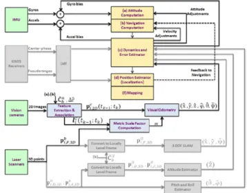
A block diagram for the methodology implemented in this research is depicted in Figure 3, with the elements related to monocular camera methods highlighted. When assessing the capabilities of each of the sensors used in the work, only the inertial sensor produces data that is solely dependent on the motion of the platform and local gravity and is more or less unaffected by its surroundings. Therefore, the inertial is chosen to be the primary sensor for this method. The mechanization integrates the measurements from GPS, the laser scanners and the monocular camera, through a complementary Kalman Filter (CKF) that estimates the errors in the inertial measurements and feeds them back to the inertial strapdown calculations. For this inertial error estimation method to function properly, pre-processing methods must be implemented that relate the sensors’ observables to the inertial measurements. The following section describes the processing techniques necessary to relate measurements from a monocular camera to measurements from the IMU. Following the discussion of these techniques, the remainder of this paper presents how these techniques are used in the broader GPS/optical/inertial mechanization, the results of testing using such an integration, and conclusions.
Figure 3. Monocular camera components of a broader mechanization.
2D MONOCULAR CAMERA METHODS
To process data from the camera we first perform feature detection and tracking of both point features and line features. Specifically, elements from Lowe's Scale Invariant Feature Transforms (SIFT) [3] are used to track point features, which are in turn used to obtain estimates of the camera’s rotational and un-scaled translational motion using structure from motion (SFM) based methods. To resolve the ambiguous scale factor, a novel scale estimation technique is employed that uses data from the
platform’s horizontally scanning laser. This technique as well as algorithms that produce a 3D visual odometry solution are presented below.
SIFT Point Feature Extraction and Association To aid in determining camera motion, SIFT has been used as a way of identifying local features that are invariant to translation, rotation, and image scaling. This technique yields 2D point features that are unique to their surroundings and readily identified and associated across a set of sequential camera images. Through the analysis of difference of Gaussian (DoG) functions computed on a multi-scale representation of an image, key locations can be identified at local maxima and minima, which are inherently located at places in the image with high variations at each scale. The larger these variations, the better the features can be identified in future images while the camera moves. Through the processes described in [4], each key location and its surroundings are analyzed resulting in a descriptive 128 element feature vector, known as a SIFT key. Example results of the SIFT key identification process are shown in Figure 4.
Figure 4. SIFT feature identification.
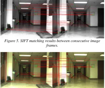
Based on the results of the SIFT feature extraction process from two image frames, a feature association function is performed using the feature vectors. For this work, a two-step procedure is implemented. First, SIFT keys are associated using the matching procedure in the "Sift for Matlab" code developed in [5]. Example results of this process are shown in Figure 5, where it can be observed that incorrectly associated features may result from this process. To remove these artifacts, inertial measurements are utilized to ensure the correctness of the associations. Using the triangulation method described in [6], prospective associations are used to crudely estimate each feature’s 3D position with respect to the previous frame. While this triangulation method yields 3D data, it is of poor quality, and is therefore only used to obtain rough approximations that are sufficient for association purposes, but insufficient for navigation purposes. Once transformed to a 3D reference frame, the projected distances of each feature are compared with one another and prospective associations that produce significantly different depths
than surrounding points are eliminated. Example results of this filtering process can be seen in Figure 6.
Figure 5. SIFT matching results between consecutive image frames.
Figure 6. Point feature association after inertial based miss-association rejection.
In future implementations, the ORB feature will be evaluated, as its performance is expected to be more than two orders of magnitude faster than SIFT [7].
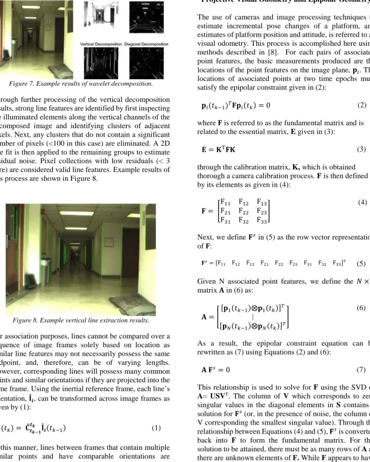
Wavelet Line Feature Extraction and Association To implement the scale factor estimation technique described in a later section, it is necessary to first extract and track vertical line features. To accomplish this, a method using wavelet transforms (WTs) was developed. In general, a WT is a multi-scale transformation that produces a time-frequency representation of a signal using “basis functions.” These bias functions are scaled and time-shifted copies of a “mother wavelet”. When applied to a 2D image, WTs can be viewed as filters operating in the x and y directions of an image. These filters may be high-pass or low-pass filters with different bandwidths. By applying either a high- or low-pass filter to both of an image’s channels (i.e., x and y directions), four sub-images are formed to represent an image approximation. For this work, a level one bi-orthogonal 1.3 wavelet was used to decompose each image. An example of the four sub-images produced by this wavelet is shown in Figure 7 along with the original image.
Figure 7. Example results of wavelet decomposition. Through further processing of the vertical decomposition results, strong line features are identified by first inspecting the illuminated elements along the vertical channels of the decomposed image and identifying clusters of adjacent pixels. Next, any clusters that do not contain a significant number of pixels (<100 in this case) are eliminated. A 2D line fit is then applied to the remaining groups to estimate residual noise. Pixel collections with low residuals (< 3 here) are considered valid line features. Example results of this process are shown in Figure 8.
Figure 8. Example vertical line extraction results. For association purposes, lines cannot be compared over a sequence of image frames solely based on location as similar line features may not necessarily possess the same endpoint, and, therefore, can be of varying lengths. However, corresponding lines will possess many common points and similar orientations if they are projected into the same frame. Using the inertial reference frame, each line’s orientation, 𝐥𝐥̂𝒊𝒊, can be transformed across image frames as given by (1):
𝐥𝐥̂𝒊𝒊(𝑡𝑡𝑘𝑘) = 𝐂𝐂�𝒕𝒕𝒌𝒌−𝟏𝟏
𝒕𝒕𝒌𝒌 𝐥𝐥̂
𝒊𝒊(𝑡𝑡𝑘𝑘−1) (1)
In this manner, lines between frames that contain multiple similar points and have comparable orientations are considered associated.
Projective Visual Odometry and Epipolar Geometry The use of cameras and image processing techniques to estimate incremental pose changes of a platform, and estimates of platform position and attitude, is referred to as visual odometry. This process is accomplished here using methods described in [8]. For each pairs of associated point features, the basic measurements produced are the locations of the point features on the image plane, 𝐩𝐩𝑖𝑖. The locations of associated points at two time epochs must satisfy the epipolar constraint given in (2):
𝐩𝐩𝑖𝑖(𝑡𝑡𝑘𝑘−1)𝑇𝑇𝐅𝐅𝐩𝐩𝑖𝑖(𝑡𝑡𝑘𝑘) = 0 (2)
where 𝐅𝐅 is referred to as the fundamental matrix and is related to the essential matrix, E given in (3):
𝐄𝐄=𝐊𝐊T𝐅𝐅𝐊𝐊 (3)
through the calibration matrix, K, which is obtained thorough a camera calibration process. F is then defined by its elements as given in (4):
𝐅𝐅= �FF1121 FF1222 FF1323
F31 F32 F33
� (4)
Next, we define 𝐅𝐅𝑠𝑠 in (5) as the row vector representation of 𝐅𝐅:
𝐅𝐅𝑠𝑠= [F11 F12 F13 F21 F22 F23 F31 F32 F33]𝑇𝑇 (5) Given N associated point features, we define the 𝑁𝑁× 9 matrix 𝐀𝐀 in (6) as: 𝐀𝐀=�[𝐩𝐩1(𝑡𝑡𝑘𝑘−1)⨂𝐩𝐩1(𝑡𝑡𝑘𝑘)] 𝑇𝑇 ⋮ [𝐩𝐩𝑁𝑁(𝑡𝑡𝑘𝑘−1)⨂𝐩𝐩𝑁𝑁(𝑡𝑡𝑘𝑘)]𝑇𝑇 � (6)
As a result, the epipolar constraint equation can be rewritten as (7) using Equations (2) and (6):
𝐀𝐀𝐅𝐅𝑠𝑠= 0 (7)
This relationship is used to solve for F using the SVD of A= USVT. The column of V which corresponds to zero
singular values in the diagonal elements in S contains a solution for 𝐅𝐅𝑠𝑠(or, in the presence of noise, the column of V corresponding the smallest singular value). Through the relationship between Equations (4) and (5), 𝐅𝐅𝑠𝑠 is converted back into F to form the fundamental matrix. For this solution to be attained, there must be as many rows of A as there are unknown elements of F. While F appears to have nine unknowns, one of its elements is guaranteed to be uniquely zero. Therefore, eight sets of matching points are required to find a unique solution to F. For this reason, this process is often known as the eight-point algorithm.
Once the eight-point algorithm is completed, the intrinsic parameters [8] of the camera are considered. These parameters are represented in the matrix K, and are infused into the fundamental matrix to form the essential matrix, E. Through application of the SVD on 𝐄𝐄=𝐔𝐔𝐔𝐔𝐕𝐕𝑇𝑇, two possible solutions for the rotation can found using (8) and (9):
𝐂𝐂𝑡𝑡𝑡𝑡𝑘𝑘𝑘𝑘+1=𝐑𝐑
𝟏𝟏=𝐔𝐔𝐖𝐖𝐕𝐕T (8)
𝐂𝐂𝑡𝑡𝑡𝑡𝑘𝑘𝑘𝑘+1=𝐑𝐑
𝟐𝟐=𝐔𝐔𝐖𝐖T𝐕𝐕T (9)
Where W is found using (10):
𝐖𝐖=�01 −01 00
0 0 1�
(10)
Two possible translations can be found as well using (11) and (12):
[∆𝐫𝐫�×] =𝐘𝐘1=𝐔𝐔𝐖𝐖𝐔𝐔𝐔𝐔T (11)
[∆𝐫𝐫�×] =𝐘𝐘2=𝐔𝐔𝐖𝐖𝐓𝐓𝐔𝐔𝐔𝐔T (12)
where Δ𝐫𝐫� is unit-length and, thus, indicates the direction in which the camera is travelling. Δ𝐫𝐫� is related to the translation ∆𝐫𝐫 through a scale factor, m, as given by (13):
∆𝐫𝐫= m ∆𝐫𝐫� (13)
Since two possible solutions exist for both the camera rotation and translation, there are four possible solutions. By considering each of the four geometric solutions and the translations and rotations that project associated point features into 3D space, the correct rotation and translation combination can be identified. When these four solutions are applied for projection purposes, only one yields a 3D point that could be physically observed by the camera.
Resolution of True Metric Scale
As the unscaled translation estimate calculated through the aforementioned visual odometry method is a unit vector, ‖∆𝐫𝐫�‖ = 1, it only indicates the most likely direction of motion of the camera. To obtain the sensor’s actual translational motion, an estimate of the scale factor, m, is requiredto determine the absolute translation ∆𝐫𝐫. This can be accomplished through techniques such as those seen in [9][10][11]. These methods use of a priori knowledge of the operational environment or measurements from other sensors. In this research effort, a new method is employed
that makes use of data provided by a horizontally scanning laser.
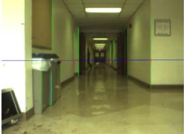
The proposed method estimates the scale in an image by identifying points in the environment that are simultaneously observed by the camera and the forward-looking laser range scanner. To enable this estimation method we must identify the correspondences between the pixels in the camera images (each defined by a direction unit vector 𝐞𝐞𝑐𝑐𝑏𝑏,𝑥𝑥,𝑦𝑦 corresponding to the row x and column y) and the laser scanner measurements (each defined by direction unit vector 𝐞𝐞𝑙𝑙𝑏𝑏,𝛼𝛼). A calibration procedure described in [1] establishes these correspondences. Given the laser range measurements, 2D features located on the scan/pixel intersections can be scaled up to 3D points. Unfortunately, extracted 2D point features are rarely illuminated by a laser scan in two consecutive frames. This can be resolved by considering the intersection of a laser scan with 2D line features rather than point features. As the laser intersects the camera frame at the same location regardless of platform motion, and the platform does not make excessive roll and pitch maneuvers, vertical line features in the image frame are preferred as they will be relatively orthogonal to the laser scan plane. Using the previously-described vertical line extraction procedure, Figure 9 shows an example image frame overlaid with the points in the image frame illuminated by the laser (indicated by a blue line) and the extracted vertical line features (indicated as green lines). Multiple intersections of 2D vertical lines with laser scan data are calculated (indicated as red points).
Figure 9. 2D vertical line and laser intersections overlaying an example image frame.
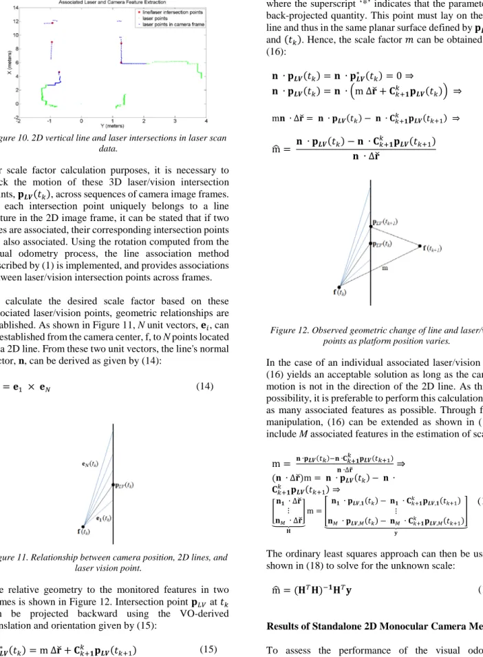
Inversely, Figure 10 depicts the location of all laser scan points in green, all laser points observable with the field-of-view (FoV) of the camera in blue, and the intersection points in red.
Figure 10. 2D vertical line and laser intersections in laser scan data.
For scale factor calculation purposes, it is necessary to track the motion of these 3D laser/vision intersection points, 𝐩𝐩𝑳𝑳𝑳𝑳(𝑡𝑡𝑘𝑘), across sequences of camera image frames. As each intersection point uniquely belongs to a line feature in the 2D image frame, it can be stated that if two lines are associated, their corresponding intersection points are also associated. Using the rotation computed from the visual odometry process, the line association method described by (1) is implemented, and provides associations between laser/vision intersection points across frames. To calculate the desired scale factor based on these associated laser/vision points, geometric relationships are established. As shown in Figure 11, N unit vectors, 𝐞𝐞𝑖𝑖, can be established from the camera center, f, to N points located on a 2D line. From these two unit vectors, the line's normal vector, n, can be derived as given by (14):
𝐧𝐧=𝐞𝐞1 × 𝐞𝐞𝑁𝑁 (14)
Figure 11. Relationship between camera position, 2D lines, and laser vision point.
The relative geometry to the monitored features in two frames is shown in Figure 12. Intersection point 𝐩𝐩𝐿𝐿𝐿𝐿 at 𝑡𝑡𝑘𝑘 can be projected backward using the VO-derived translation and orientation given by (15):
𝐩𝐩𝑳𝑳𝑳𝑳∗ (𝑡𝑡𝑘𝑘) = m ∆𝐫𝐫�+𝐂𝐂𝑘𝑘+𝟏𝟏𝑘𝑘 𝐩𝐩𝑳𝑳𝑳𝑳(𝑡𝑡𝑘𝑘+1) (15)
where the superscript ‘*’ indicates that the parameter is a back-projected quantity. This point must lay on the same line and thus in the same planar surface defined by 𝐩𝐩𝑳𝑳𝑳𝑳(𝑡𝑡𝑘𝑘) and (𝑡𝑡𝑘𝑘). Hence, the scale factor 𝑚𝑚 can be obtained using (16):
𝐧𝐧 ∙ 𝐩𝐩𝑳𝑳𝑳𝑳(𝑡𝑡𝑘𝑘) =𝐧𝐧 ∙ 𝐩𝐩𝑳𝑳𝑳𝑳∗ (𝑡𝑡𝑘𝑘) = 0⇒
𝐧𝐧 ∙ 𝐩𝐩𝑳𝑳𝑳𝑳(𝑡𝑡𝑘𝑘) =𝐧𝐧 ∙ �m ∆𝐫𝐫�+𝐂𝐂𝑘𝑘+𝟏𝟏𝑘𝑘 𝐩𝐩𝑳𝑳𝑳𝑳(𝑡𝑡𝑘𝑘)� ⇒ m𝐧𝐧 ∙ ∆𝐫𝐫�= 𝐧𝐧 ∙ 𝐩𝐩𝑳𝑳𝑳𝑳(𝑡𝑡𝑘𝑘)− 𝐧𝐧 ∙ 𝐂𝐂𝑘𝑘+𝟏𝟏𝑘𝑘 𝐩𝐩𝑳𝑳𝑳𝑳(𝑡𝑡𝑘𝑘+1) ⇒
m� = 𝐧𝐧 ∙ 𝐩𝐩𝑳𝑳𝑳𝑳(𝑡𝑡𝑘𝑘)− 𝐧𝐧𝐧𝐧 ∙ ∆𝐫𝐫�∙ 𝐂𝐂𝑘𝑘𝑘𝑘+𝟏𝟏𝐩𝐩𝑳𝑳𝑳𝑳(𝑡𝑡𝑘𝑘+1) (16)
Figure 12. Observed geometric change of line and laser/vision points as platform position varies.
In the case of an individual associated laser/vision point, (16) yields an acceptable solution as long as the camera's motion is not in the direction of the 2D line. As this is a possibility, it is preferable to perform this calculation using as many associated features as possible. Through further manipulation, (16) can be extended as shown in (17) to include M associated features in the estimation of scale:
m = 𝐧𝐧∙𝐩𝐩𝑳𝑳𝑳𝑳(𝑡𝑡𝑘𝑘)−𝐧𝐧∙𝐂𝐂𝑘𝑘+𝟏𝟏𝑘𝑘 𝐩𝐩𝑳𝑳𝑳𝑳(𝑡𝑡𝑘𝑘+1) 𝐧𝐧∙∆𝐫𝐫� ⇒ (𝐧𝐧 ∙ ∆𝐫𝐫�)m = 𝐧𝐧 ∙ 𝐩𝐩𝑳𝑳𝑳𝑳(𝑡𝑡𝑘𝑘)− 𝐧𝐧 ∙ 𝐂𝐂𝑘𝑘+𝟏𝟏𝑘𝑘 𝐩𝐩𝑳𝑳𝑳𝑳(𝑡𝑡𝑘𝑘+1)⇒ �𝐧𝐧𝟏𝟏⋮∙ ∆𝐫𝐫� 𝐧𝐧𝑀𝑀 ∙ ∆𝐫𝐫� � ������� 𝐇𝐇 m =� 𝐧𝐧𝟏𝟏 ∙ 𝐩𝐩𝑳𝑳𝑳𝑳,𝟏𝟏(𝑡𝑡𝑘𝑘)−𝐧𝐧𝟏𝟏 ∙ 𝐂𝐂𝑘𝑘+𝟏𝟏 𝑘𝑘 𝐩𝐩 𝑳𝑳𝑳𝑳,𝟏𝟏(𝑡𝑡𝑘𝑘+1) ⋮ 𝐧𝐧𝑀𝑀 ∙ 𝐩𝐩𝑳𝑳𝑳𝑳,𝑀𝑀(𝑡𝑡𝑘𝑘)−𝐧𝐧𝑀𝑀 ∙ 𝐂𝐂𝑘𝑘+𝟏𝟏𝑘𝑘 𝐩𝐩𝑳𝑳𝑳𝑳,𝑀𝑀(𝑡𝑡𝑘𝑘+1) � ��������������������������� 𝐲𝐲 (17)
The ordinary least squares approach can then be used as shown in (18) to solve for the unknown scale:
m� = (𝐇𝐇𝑇𝑇𝐇𝐇)−𝟏𝟏𝐇𝐇𝑇𝑇𝐲𝐲 (18)
Results of Standalone 2D Monocular Camera Methods To assess the performance of the visual odometry processes, multiple experiments were conducted. The results of two tests are discussed in this paper, and further
results can be found in [1]. During each test, the visual odometry results for rotation, shown in blue, were easily evaluated through comparison with the platform’s inertially-measured rotation, displayed in red. The rotational results for each sensor were decomposed into the Euler angles: pitch, roll and yaw with respect to an established navigation frame. Unfortunately, the inertial sensor itself cannot be used to evaluate the visual odometry translation results due to relatively large inertial drift in the sensor measurements. As no independent measurements were available to evaluate translation with high precision, the truth reference was established by accurately measuring the actual paths taken during each flight.
For one test, the platform was flown along a feature-rich hallway. Results of the attitude estimation are shown in Figure 13. During the 113 second flight, pitch and yaw remained consistent with the inertial solution to less than 3°, while roll remained within 5°.
d
Figure 13. Visual odometry attitude estimation during a test flight traversing a hallway.
With respect to translational motion estimation produced through the flight, Figure 14 shows that the cross-track error of the estimated trajectory with respect to the reference trajectory deviated by no more than 25cm, however, the along-track position deviated by as a large as 40 cm.
Figure 14. Visual odometry path determination during a test flight traversing a hallway.
A second test flight was conducted traversing a rectangular indoor hallway loop. In contrast to the relatively simple
first test, this test contained translation in multiple dimensions, large heading changes, as well as an increase in duration of flight. Moreover, this test allowed for evaluation of the eight point algorithm and scale estimation method in the presence of rapid scene changes.
The attitude estimation results for the second test are shown in Figure 15. Throughout data collection, the maximum separation between the inertial and vision based attitude estimators for pitch, roll and yaw was 9°,19°, and 14°, respectively. Upon comparison to the first test, the maximum attitude errors were larger. There are multiple reasons for this increase. First, the duration of experiment 2 was more than double that of the previous experiment. Errors accumulate as a function as time due to integration of residual bias errors, so increasing flight duration will increase cumulative error. Next, the looping path observed throughout this test cause the eight-point algorithm and scale estimation procedures to quickly adapt to differing scenery. Drastic scene changes (i.e. turning a corner) increase the difficulty of feature association between frames. This directly affects the procedures used for visual odometry in an adverse manner. Finally, there are situations in this flight where features are sparse. In general, a decrease in features will cause a decrease in the estimation capabilities of visual odometry.
Figure 15. Visual odometry attitude estimation while traveling around an indoor loop.
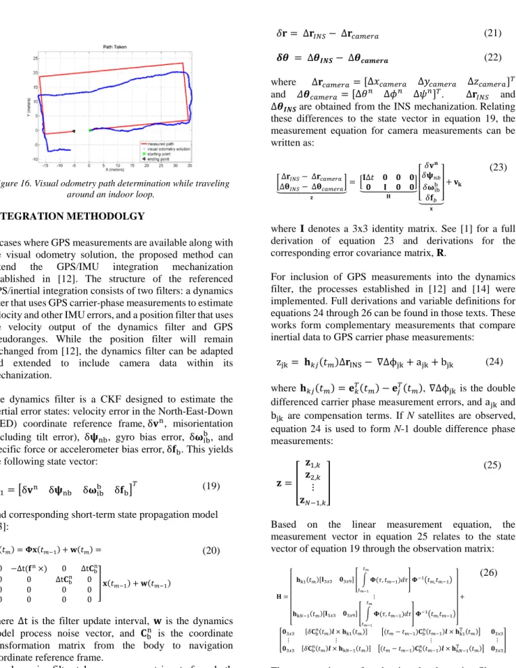
The visual odometry path calculated for experiment 2 can be observed in Figure 16. In this figure, it is shown that the estimated length of each of the 4 straight legs of the rectangular loop matches to within 2 meters of the measured hallway lengths. This implies that the scale estimation technique is working reasonably well. As for the estimated translational directionality produced by the eight-point algorithm, the first two legs of the loop never divert from the measured path by more than 2 meters. Unfortunately, the third leg diverts by 5 meters. This is most likely due to a lack of well dispersed features in that specific hallway. The cumulative error contained in the third linear leg of the loop also makes evaluation of the final leg difficult. However, if previous errors are removed, the final leg appears to match the measured path well. In total, the landing position calculated through visual odometry is 6.5 meters away from the measured end of the trial.
Figure 16. Visual odometry path determination while traveling around an indoor loop.
INTEGRATION METHODOLGY
In cases where GPS measurements are available along with the visual odometry solution, the proposed method can extend the GPS/IMU integration mechanization established in [12]. The structure of the referenced GPS/inertial integration consists of two filters: a dynamics filter that uses GPS carrier-phase measurements to estimate velocity and other IMU errors, and a position filter that uses the velocity output of the dynamics filter and GPS pseudoranges. While the position filter will remain unchanged from [12], the dynamics filter can be adapted and extended to include camera data within its mechanization.
The dynamics filter is a CKF designed to estimate the inertial error states: velocity error in the North-East-Down (NED) coordinate reference frame,δ𝐯𝐯n, misorientation (including tilt error), δ𝛙𝛙nb, gyro bias error, δ𝛚𝛚ibb, and specific force or accelerometer bias error,δ𝐟𝐟b. This yields the following state vector:
𝐱𝐱1=�δ𝐯𝐯n δ𝛙𝛙nb δ𝛚𝛚ibb δ𝐟𝐟b�𝑇𝑇 (19)
And corresponding short-term state propagation model [13]: 𝐱𝐱(𝑡𝑡𝑚𝑚) =𝚽𝚽𝐱𝐱(𝑡𝑡𝑚𝑚−1) +𝐰𝐰(𝑡𝑡𝑚𝑚) = � 0 −∆t(𝐟𝐟n×) 0 ∆t𝐂𝐂 b n 0 0 ∆t𝐂𝐂bn 0 0 0 0 0 0 0 0 0 � 𝐱𝐱(𝑡𝑡𝑚𝑚−1) +𝐰𝐰(𝑡𝑡𝑚𝑚−1) (20)
where ∆t is the filter update interval, 𝐰𝐰 is the dynamics model process noise vector, and 𝐂𝐂bn is the coordinate transformation matrix from the body to navigation coordinate reference frame.
The dynamics filter takes measurement inputs from both GPS and the visual odometry solution. The vision-based measurement is formed by taking the difference between the position change as computed through visual odometry and the inertial navigation system (INS), or:
𝛿𝛿𝐫𝐫= ∆𝐫𝐫𝐼𝐼𝑁𝑁𝐼𝐼− ∆𝐫𝐫𝑐𝑐𝑐𝑐𝑚𝑚𝑐𝑐𝑐𝑐𝑐𝑐 (21)
𝜹𝜹𝜹𝜹 = ∆𝜹𝜹𝑰𝑰𝑰𝑰𝑰𝑰− ∆𝜹𝜹𝒄𝒄𝒄𝒄𝒄𝒄𝒄𝒄𝒄𝒄𝒄𝒄 (22)
where Δ𝐫𝐫𝑐𝑐𝑐𝑐𝑚𝑚𝑐𝑐𝑐𝑐𝑐𝑐= [Δ𝑥𝑥𝑐𝑐𝑐𝑐𝑚𝑚𝑐𝑐𝑐𝑐𝑐𝑐 Δ𝑦𝑦𝑐𝑐𝑐𝑐𝑚𝑚𝑐𝑐𝑐𝑐𝑐𝑐 Δ𝑧𝑧𝑐𝑐𝑐𝑐𝑚𝑚𝑐𝑐𝑐𝑐𝑐𝑐]𝑇𝑇 and 𝛥𝛥𝜹𝜹𝑐𝑐𝑐𝑐𝑚𝑚𝑐𝑐𝑐𝑐𝑐𝑐 = [∆𝜃𝜃𝑛𝑛 ∆𝜙𝜙𝑛𝑛 ∆𝜓𝜓𝑛𝑛]𝑇𝑇. Δ𝐫𝐫𝐼𝐼𝑁𝑁𝐼𝐼 and
∆𝜹𝜹𝑰𝑰𝑰𝑰𝑰𝑰are obtained from the INS mechanization.Relating
these differences to the state vector in equation 19, the measurement equation for camera measurements can be written as: � ∆𝐫𝐫𝐼𝐼𝑁𝑁𝐼𝐼− ∆𝐫𝐫𝑐𝑐𝑐𝑐𝑚𝑚𝑐𝑐𝑐𝑐𝑐𝑐 ∆𝛉𝛉𝐼𝐼𝑁𝑁𝐼𝐼−∆𝛉𝛉𝑐𝑐𝑐𝑐𝑚𝑚𝑐𝑐𝑐𝑐𝑐𝑐� ������������� 𝐳𝐳 = �𝐈𝐈∆𝑡𝑡 𝟎𝟎 𝟎𝟎 𝟎𝟎�����������𝟎𝟎 𝐈𝐈 𝟎𝟎 𝟎𝟎� 𝐇𝐇 ⎣⎢ ⎢ ⎡𝛿𝛿𝛙𝛙𝛿𝛿𝐯𝐯𝑛𝑛𝑏𝑏𝐧𝐧 𝛿𝛿𝛚𝛚ibb 𝛿𝛿𝐟𝐟𝑏𝑏 ⎦ ⎥ ⎥ ⎤ ����� 𝐱𝐱 +𝐯𝐯𝐤𝐤 (23)
where I denotes a 3x3 identity matrix. See [1] for a full derivation of equation 23 and derivations for the corresponding error covariance matrix, R.
For inclusion of GPS measurements into the dynamics filter, the processes established in [12] and [14] were implemented. Full derivations and variable definitions for equations 24 through 26 can be found in those texts. These works form complementary measurements that compare inertial data to GPS carrier phase measurements:
zjk= 𝐡𝐡𝑘𝑘𝑘𝑘(𝑡𝑡𝑚𝑚)∆𝐫𝐫INS− ∇Δϕjk+ ajk+ bjk (24)
where 𝐡𝐡𝑘𝑘𝑘𝑘(𝑡𝑡𝑚𝑚) =𝐞𝐞𝑘𝑘𝑇𝑇(𝑡𝑡𝑚𝑚)− 𝐞𝐞𝑘𝑘𝑇𝑇(𝑡𝑡𝑚𝑚), ∇Δϕjk is the double differenced carrier phase measurement errors, and ajk and
bjk are compensation terms. If N satellites are observed,
equation 24 is used to form N-1 double difference phase measurements: 𝐳𝐳=� 𝐳𝐳1,𝑘𝑘 𝐳𝐳2,𝑘𝑘 ⋮ 𝐳𝐳𝑁𝑁−1,𝑘𝑘 � (25)
Based on the linear measurement equation, the measurement vector in equation 25 relates to the state vector of equation 19 through the observation matrix:
𝐇𝐇= ⎣ ⎢ ⎢ ⎢ ⎢ ⎢ ⎢ ⎡ 𝐡𝐡 k1(𝑡𝑡𝑚𝑚)[𝐈𝐈3𝑥𝑥3 𝟎𝟎3𝑥𝑥9]� � 𝚽𝚽(𝜏𝜏, 𝑡𝑡𝑚𝑚 𝑡𝑡𝑚𝑚−1 𝑡𝑡𝑚𝑚−1)𝑑𝑑𝜏𝜏� 𝚽𝚽−1�𝑡𝑡𝑚𝑚,𝑡𝑡𝑚𝑚−1� ⋮ 𝐡𝐡k𝑁𝑁−1(𝑡𝑡𝑚𝑚)[𝐈𝐈3𝑥𝑥3 𝟎𝟎3𝑥𝑥9]� � 𝚽𝚽(𝜏𝜏, 𝑡𝑡𝑚𝑚 𝑡𝑡𝑚𝑚−1 𝑡𝑡𝑚𝑚−1)𝑑𝑑𝜏𝜏� 𝚽𝚽−1�𝑡𝑡𝑚𝑚,𝑡𝑡𝑚𝑚−1� ⎦ ⎥ ⎥ ⎥ ⎥ ⎥ ⎥ ⎤ + (26) �𝟎𝟎3𝑥𝑥3 [𝛿𝛿𝐂𝐂b n(𝑡𝑡 𝑚𝑚)𝒍𝒍×𝐡𝐡k1(𝑡𝑡𝑚𝑚)] �(𝑡𝑡𝑚𝑚− 𝑡𝑡𝑚𝑚−1)𝐂𝐂bn(𝑡𝑡𝑚𝑚−1)𝒍𝒍×𝐡𝐡k1T(𝑡𝑡𝑚𝑚)� 𝟎𝟎3𝑥𝑥3 ⋮ ⋮ ⋮ ⋮ 𝟎𝟎3𝑥𝑥3 [𝛿𝛿𝐂𝐂bn(𝑡𝑡𝑚𝑚)𝒍𝒍×𝐡𝐡k𝑁𝑁−1(𝑡𝑡𝑚𝑚)] �(𝑡𝑡𝑚𝑚− 𝑡𝑡𝑚𝑚−1)𝐂𝐂bn(𝑡𝑡𝑚𝑚−1)𝒍𝒍×𝐡𝐡k𝑁𝑁−1T (𝑡𝑡𝑚𝑚)� 𝟎𝟎3𝑥𝑥3 �
The error estimates found using the dynamics filter are directly fed back to the attitude (a) and navigation (b) estimators of the inertial mechanization shown in Figure 3.
The position estimator in Figure 3 is a simple Kalman Filter implementation that uses the outputs of the corrected inertial from the previously discussed dynamics filter and satellite pseudoranges. This state vector is equal to the North-East-Down (NED) position, 𝐫𝐫𝑛𝑛. Since the velocity output of the dynamics filter is accurately known, it can be used as a forcing function:
𝐱𝐱(tm) = 𝐱𝐱(tm−1) +𝐮𝐮(tm−1) +𝐰𝐰(tm) (27)
where 𝐮𝐮(𝑡𝑡𝑚𝑚−1) is the integrated velocity from the dynamics filter (e.g. 𝐮𝐮(𝑡𝑡𝑚𝑚−1) =𝐯𝐯�(𝑡𝑡𝑚𝑚−1)Δ𝑡𝑡). The measurements can be obtained from a straight forward pseudorange based position solution. As previously stated, this filter initializes at the origin of an established local navigation frame. However, the local frame is relative and an absolute reference frame is desired. Given the above mechanization, if four or more pseudoranges are available, an absolute position calculation can be made. When an absolute position is obtained, the reference frame for the filter is converted from a local NED frame to an absolute Earth Centered Earth Fixed (ECEF) frame. Once conversion to this reference frame is made, the filter proceeds to output absolute positions regardless of the number of pseudorange measurements. Essentially, if an absolute position is ever obtained, then all of the filter outputs will correspondingly be in the absolute frame (e.g. ECEF).
RESULTS
To evaluate the proposed algorithms, data was collected through multiple flights of the hexacopter platform shown in Figure 2 through a structured indoor and outdoor environment including transitions between these two environments. The availability of GPS measurements in these environments ranged from fully denied, to substantially degraded, to enough observables for a full solution. The results of one test flight are discussed in this section. Further results along with a more detailed description of the operational environment can be found in [1]. Apart from the data collections with the hexacopter, truth reference maps were created for the indoor operational environment and used for evaluation of the described processes.
The results of the full GPS/inertial/laser/camera integrated solution described in Figure 3 are shown in an NED frame in Figure 17. The truth reference of the environment, depicted in red (derived from a terrestrial laser scanner), is compared to the flight path obtained from the EKF, displayed in blue. The estimated flight trajectory constantly remains within in hallway truth model, indicating sub-meter level performance. Furthermore, based on an extension of this work for environmental laser mapping [1] produced from the EKF, combined with the accuracy of the
map, it is further reinforced that sub-meter level navigation performance is obtained.
Figure 17. Path compared to 2D reference map. During portions of the described data collection, there was enough visibility (> 3 satellites) to calculate a GPS position. The availability of GPS measurements to the position estimation portion of the filter allowed for geo-referencing of the produced flight path and 3D map. Figure 18 displays the geo-referenced flight path based on the integration filter superimposed on Google Earth™ on the left, while the standalone GPS solution based on pseudoranges only is plotted on the right. The geo-referenced path correctly displays the platform passing through Stocker Center, the Ohio University engineering building.
Figure 18. (a) Left: EKF produced path; (b) Right: standalone GPS path.
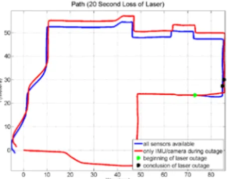
To demonstrate the contributions of the monocular camera to the above results, laser measurements were removed from the solution for a 20 second period where GPS was unavailable. During the 20 second removal of laser data, the system is forced to operate on integration between visual odometry measurements and the IMU. The cumulative effect caused by this situation can be observed in Figure 19. After coasting on an IMU/camera solution for 20 seconds, the path is subsequently altered by 3 meters, as opposed to the solution with all sensors.
Figure 19. Effect of losing GPS and lasers for 20 seconds. To further emphasize the contribution of the visual odometry component, both the laser and camera were removed from the integration for the same 20 second period. During this time frame the EKF is forced to coast on calibrated inertial measurements. The effect of losing all secondary sensors for a 20 second period can be observed in Figure 20. During the forced sensor outage, a 45 meter cumulative difference is introduced between the path using all sensors and the path with denied sensors. Through comparison of the results shown in Figure 19 and Figure 20. The contribution of monocular camera data can be isolated. When the EKF was forced to operate for 20 seconds using an IMU/camera solution, 3 meters of error were introduced. This is significantly smaller than the 45 meters of error observed when using only the inertial for the same period. Thus, the camera is shown to provide stability to the EKF when neither the laser nor GPS are available.
Figure 20. Effect of coasting on the IMU for 20 seconds. SUMMARY AND CONCLUSIONS
This paper presented an implementation of a monocular camera-based visual odometry method, a unique wavelet line extraction procedure, a novel scale estimation process, and a 6DOF pose estimation technique that integrates GPS, IMU and camera measurements into a single solution. Each of the presented methods was tested and evaluated using data collected by a specifically designed hexacopter. Through this data it was shown that the visual odometry techniques produced reasonably good attitude estimation and are effective at constraining inertial drift when other
sensors are not available. The inclusion of camera measurements to the discussed integrated solution resulted in increases in the accuracy, availability, continuity and reliability of the system.
REFERENCES
[1] Dill, E., “GPS/Optical/Inertial Integration for 3D Navigation and Mapping Using Multi-copter Platforms,” Ph.D. Dissertation, Ohio University, December, 2014.
[2] Kopardekar, P., Rios, J., Prevot, T., Johnson, M., Jung, J., & Robinson, J., “Unmanned aircraft system traffic management (utm) concept of operations,” 16th AIAA Aviation Technology, Integration, and Operations Conference, AIAA Aviation, 2016. [3] Lowe, D.G. “Object Recognition from Local
Scale-Invariant Features,” Computer Science Department, University of British Columbia, Vancouver, Canada, 1999.
[4] Lowe, D. “Distinctive image features from scale-invariant keypoints,” International Journal of Computer Vision, vol. 60, pp. 91–110, 2004.
[5] Vedaldi, A.,
http://www.robots.ox.ac.uk/~vedaldi/code/sift.html l , University of California, Los Angeles(UCLA), 2006.
[6] Zisserman, A. and Hartley, R., "Multiple View Geometry in Computer Vision," CambridgeUniversity Press, 2003.
[7] Rublee, E., V. Rabaud, K. Konolige, and G. Bradski, “ORB: an efficient alternative to SIFT or SURF,” in
IEEE International Conference on Computer Vision
(ICCV), Barcelona, Spain, November 2011, pp.
2564–2571
[8] Ma, Y., Soatto, S., Kosecka, J., and Sastry, S.S.,An Invitation to 3-D Vision, Springer Science and Business Media, Inc., New York, 2004.
[9] Soloviev, A., Gans,N., Uijt de Haag, M., “Integration of Video Camera with 2D Laser Scanner for 3D Navigation,” Proceedings of the 2009 International Technical Meeting of the Institute of Navigation, January 26 - 28, 2009, Anaheim,CA, pp. 767 – 776.
[10] Engel, J., Strum, J., Cremers, D., "Scale-Aware Navigation of a Low-Cost Quadrocopter with a Monocular Camera", Robotics and Autonomous Systems (RAS), 2014.
[11] Kitt, B., Rehder, J., Chambers, A., Schonbein, M., Lategahn, H., Singh, S., "Monocular Visual Odometry using a Planar Road Model to Solve Scale Ambiguity", European Conference on Mobile Robotics, 2011.
[12] Farrell, J.L., “GNSS Aided Navigation and Tracking,” American Literary Press, 2007.
[13] Wendel, J., Meister, O. Monikes, R., Trommer, G.F., "Time-Differenced Carrier Phase
Measurements for Tightly Coupled GPS/INS Integration," Proceedings of the ION/IEEE Position Location and Navigation Symposium PLANS, pp. 54-60 (2006).
[14] Uijt de Haag, M., van Graas, F., Coherent GPS/Inertial Notes, Cedar Rapids, IA, August 4, (2010).