An open benchmark implementation for multi-CPU multi-GPU pedestrian detection in automotive systems

(1)

An Open Benchmark Implementation for Multi-CPU

Multi-GPU Pedestrian Detection in Automotive Systems

Matina Maria Trompouki∗, Leonidas Kosmidis†, Nacho Navarro†,∗

∗

Universitat Polit`ecnica de Catalunya †Barcelona Supercomputing Center (BSC)

Abstract—Modern and future automotive systems incorporate several Advanced Driving Assistance Systems (ADAS). Those systems require significant performance that cannot be provided with traditional au-tomotive processors and programming models. Multicore CPUs and Nvidia GPUs using CUDA are currently considered by both automotive industry and research community to provide the necessary computational power. However, despite several recent published works in this domain, there is an absolute lack of open implementations of GPU-based ADAS software, that can be used for benchmarking candidate platforms. In this work, we present a multi-CPU and GPU implementation of an open implementation of a pedestrian detection benchmark based on the Viola-Jones image recognition algorithm. We present our optimization strategies and evaluate our implementation on a multiprocessor system featuring multiple GPUs, showing an overall 88.5× speedup over the sequential version.

I. INTRODUCTION

Modern automotive systems are getting increasingly complex every year. In particular, each generation contains more and more Advanced Driving Assistance Systems (ADAS), in order to achieve the mile-stones set by car manufacturing companies in their roadmap towards self-driving cars [10].

However, the current hardware platforms used in the automotive domain cannot satisfy the high performance requirements of future ADAS systems. The reason is that those systems are typically micro-controllers designed to comply with the strictest timing, reliability and safety requirements imposed by automotive standards such as ISO26262 [9].

As a consequence, both industry and academia have started ex-ploring alternative architectures that can provide the performance needed for these sophisticated features [13]. Multiprocessor systems and General purpose Graphics Processing Units (GPGPUs) are a promising candidate platform. Nvidia already designs embedded development kits which are promoted for use in automotive, while Qualcomm, which designs both mobile CPUs and GPUs, has recently entered strongly in the automotive domain after the acquisition of NXP. In addition, other embedded design companies with mobile GPU designs in their portfolio (ARM, Imagination Technologies and others) can offer solutions for the automotive market, which increases significantly the available number of potential candidate platforms for ADAS systems.

However, none of those platforms are already certified as ASIL-D (the highest integrity level in automotive systems) according to ISO26262 in order to be able to be used in production cars. The significant effort and cost to obtain such certification can only be justified by customer interest in purchasing large quantities of those platforms.

On the other hand, the interested parties that can create such a market demand – automotive industries and academia – lack open ADAS applications that can be used in order to benchmark the available platforms and decide which ones match their requirements

and could serve as a basis for the designs of their products. This is counter-intuitive considering that significant research has been performed recently by both agents, but it has been always considering closed-source in house developments focusing on specific hardware. In this paper, we try to bridge this gap in the literature, by presenting the design, implementation and evaluation of an open source ADAS application based on multiple CPUs and GPUs. Our baseline CPU implementation is based on an open pedestrian detec-tion case study using the Viola-Jones detecdetec-tion algorithm, developed by Thales Group within the FP7 project TERAFLUX and shared via the HiPEAC network of excellence with research institutes worldwide [14].

Our baseline application implements an object recognition task, which is a common element in ADAS systems. Despite that other computer vision and deep learning algorithms with higher detection accuracy have been proposed in the literature, all those algorithms have a similar structure with our application. Finally, our multi-CPU and multi-GPU implementation is distributed in open source form [15], retaining the same license as the original application. Therefore it is a representative application that can serve as a benchmark for future ADAS oriented automotive architectures.

Although our implementation is based on a non-proprietary code base, without using advanced state-of-the-art detection algorithms and it is released as open source, the achieved performance in our platform outperforms non-public implementations with similar characteristics, achieving real-time performance.

II. BACKGROUND

A. Features

Viola-Jones method [16][17] is an effective object recognition algorithm, that was originally proposed for face detection. The algorithm is based on a set of features, which are based on Haar wavelets. Haar wavelet is a certain sequence of rescaled ”square-shaped” functions, which together form a wavelet family. In two dimensions, a square wave is a pair of adjacent rectangles, one light and one dark.

A feature is used to detect the presence or not of a certain pattern. To achieve this, the value of the feature is evaluated with the following formula:

value=X(pixel values in white region)−

X

(pixel values in black region)

This value is compared with a threshold, provided by the classifier. If the value of the feature is higher than the threshold, the feature is considered present.

© 2017 IEEE. Personal use of this material is permitted. Permission from IEEE must be obtained for all other uses, in any current or future media, including reprinting/ republishing this material for advertising or promotional purposes, creating new collective works, for resale or redistribution to servers or lists, or reuse of any copyrighted component of this work in other works.

(2)

B. Integral Image

The Viola-Jones algorithm requires a large number of features, of many different scales and different kinds to be computed very rapidly, making it extremely computationally intensive. For this reason the concept ofintegral imagewas introduced [16][17], which is an intermediate representation of the image, in order to reduce the amount of calculations required to compute the value of a feature. This way we can detect a feature or determine its absence significantly faster.

The value of each pixel in the integral image contains the sum of all the pixel values above and to the left of the concerned pixel of the original image. Given the integral image, the evaluation of each feature can be performed by adding and subtracting values from the vertices that define the dark and white square regions of the feature. Since the number of regions in each feature is very small, the computation is very fast. We refer the interested reader to the above seminal works for more details.

C. Classification

Even though the features can be computed very efficiently, the number of possible features is very large, given the fact that there are several types of them and they are scaled and shifted across all possible combinations. In order to ensure fast classification, Viola-Jones as well as more advanced machine learning classification algorithms, has a structure that allows to exclude the presence of most features quickly and only look for a few critical features.

The Viola and Jones method combines a series of classifiers as a filter chain calledclassifier cascade. The order of filters in the cascade is based on their weight importance. The more heavily weighted filters come first, to eliminate non-detected image regions as quickly as possible. A positive result from the first classifier triggers the evaluation of a second classifier, a positive result from the second classifier triggers a third classifier and so on. A negative result at any point leads to the immediate rejection of the subregion and it is classified as ”Not Found”. The image subregion that makes it through the entire cascade is classified as ”Found”.

III. APPLICATION STRUCTURE

Our baseline code is based on a pedestrian detection application that was adapted from the OpenCV library [11] by the Thales group and it was used as a reference application in the FP 7 funded project TERAFLUX [1]. Additionally, this application is part of the Task Force of HiPEAC as a representative of its respective domain.

The algorithm used implements the Viola-Jones method written in C. The application takes 2 files as input: a classifier description and an image file. Each of the weak classifiers forms a stage and it is made up by simple features. The higher the stage of the classifier, the more complex it gets, which means that contains more features, whose number is increased exponentially with the stage. The image file contains a picture to which the detection is performed.

The application consists of two main parts. In the first one, the initial image is transformed to two intermediate representations (integral images) and in the second one, the detection takes place.

The first part of the application has two paths of execution, both starting from the input image. The first path is to compute the integral image from the input image, while the second path computes the DotSquare image (which is the square of all the pixel values) and then its integral image. Both of these paths lead to the classification phase where it is checked whether there is detection or absence of the features selected by the learning algorithm. Finally the image is written to a file, with the detected person highlighted.

read input image

compute intermediate representation images for each scale {

mark all locations as found for each subregion {

for each stage {

if feature_value < threshold {

mark the location not found break } else if stage == last_stage found++ } } if found {

for each subregion {

if location marked as found

reduce number of detections in a given range }

}

store number of detections for each scale }

delete detections which are too close highlight detection and write the image

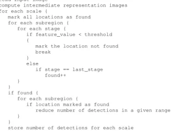
Fig. 1: High-Level Sequential Application Pseudocode.

As we can see in the pseudocode of the application in Figure 1, the detection phase starts with the smallest scale and selects a subwindow of the picture to check it for detection. Then for each stage of the classifier, takes its features, magnifies them according to the scale and checks their presence based on the threshold, as we described in the previous Section. In case of absence, the next stages of the classifier are not checked. If the last stage of the classifier is reached, then a detection has been successful in this scale.

Next, multiple detections in nearby regions are merged together in a single detection. Finally the process is completed for any combination of scales and subwindows.

A more detailed description of the application can be found in [1], [2] and [3].

IV. BENCHMARKPARALLELIZATION

First we ported the code to C++ and fixed minor bugs, regarding conversions from integer to floating point. In order to have a correct view of the performance bottlenecks of the original application, we performed profiling. This step revealed the parts of the application in which the majority of the execution time was spent and that could be effectively programmed into CUDA.

A. Classifier memory transformation

The classifier cascade is one of the most important data structures of the application, since the entire Viola-Jones algorithm is built on top of it.

The data structure comprises a hierarchical organization of nu-merous dynamically allocated nested structures linked with pointers, as depicted in the left part of Figure 2. In particular, the classifier cascade consists of an array of stage classifiers, each stage classifier of an array of classifiers, each one of them holds the set of features used for the detection, and each of them the details of the rectangles. Although this organization eases programmer’s access in its various fields, it suffers from some important disadvantages which make it inappropriate for use in a distributed memory environment as GPU computing:

(3)

1) The smaller data structures of the classifier are dynamically allocated and as a consequence, they are scattered in various locations in memory. Therefore, a naive straightforward GPU implementation based on this classifier implementation, would require many small DMA transfers, one per each individual structure. This would force the CPU to spend time setting up each short-lived DMA transfer, instead of being able to perform useful work.

2) Since host and GPU memory spaces are different, pointers from one memory space are not are not valid in the other one. In order to maintain the links between the data structures, all pointers need to be updated. In a naive implementation, this would require to perform a memory transfer to the appropriate location in the GPU, with the value of a pointer returned by the device’s memory allocation function, for each allocated structure. Since these memsets would be tiny (64bit, a size of a GPU pointer), CPU would be busy setting up a set of transfers, making matters worse.

3) Dynamic memory allocation on GPU is an expensive operation, because it requires a call to the operating system, therefore it is preferable to minimize the number of these requests. 4) Small allocations can lead to fragmentation of the address

space, which can increase the cost of large subsequent requests. This happens because the GPU memory allocator may try to reuse chunks of memory that lie between already allocated chunks.

For all the above reasons, it is clear that the organization of the classifier was needed to be modified in order to suit better the GPU programming model.

The primary idea of our modification was to allocate a single chunk of memory and partition it internally to represent the same structure. This is possible because the size of each structure is known a priori, as well as the number of structures in each level of the hierarchy. Therefore, the addresses of the various structures, which are needed to establish the links between them, can be computed as a function of the sizes and their relative position in the structure.

This way we could ensure that all the smaller data structures that comprise the classifier are allocated in contiguous memory locations. As consequence, the whole classifier structure can be transferred to the GPU memory with a single DMA transfer, which can be completed much faster than by a series of small DMA requests. Moreover the cost of a single allocation is significantly lower than many smaller ones and in addition it prevents fragmentation.

However, there there was still a challenge to be solved: since the classifier is copied in its entirety from the host memory, the pointer values are not valid anymore, since they belong to a different address space. In order to address this situation we performed a trick based on a simple observation: the relative offsets between the starting address of the classifier and each structure in it remain the same. Therefore, each pointer can be adjusted as follows:

device ptr = device classifier start+

(host classifier start - host ptr)

The advantage over the naive implementation described earlier, is that these updates can be performed in parallel by a kernel running directly in the GPU. This way there is no need for the CPU to do the same job serially, with a lot of costly small DMA transfers, instead of spending this time performing useful work.

.. . .. . .. . .. . .. . .. . cascade feature classifier stage

Original layout Transformed layout

Fig. 2: Classifier memory transformation.

B. Kernels

We implemented three kernels in order to compute the inter-mediate image representations used by the classification phase. In our implementation we took care to achieve memory coalescing, so that neighboring threads access neighboring locations. This way, the DRAM bandwidth is better utilized, because all the requests performed by the 32 threads of a warp at once, are satisfied with a single DRAM burst.

During the classification, the image is scanned at 30 different scales, starting with a very small window size (at a size of 36×18 pixels), which is incremented 10% from the previous one. Each thread is assigned a sub-window and calculates all the features of all stages. Note that compared to previous GPU works, we launch all the threads in parallel, for all the different scales. A thread continues to work on a sub-window for all the remaining stages, even if there is a fail in an earlier stage. Although this would penalize the performance in sequential execution in the CPU, this is not true for the GPU. This happens for two reasons: first, we avoid divergence between threads and second all threads are synchronized before processing the detections. In the final step, a rectangle is drawn around the detected person.

C. Scales - Stages Loop Interchange

In the previous Section, we described how the detection takes place in the original application using the classifier. The selected subwindow for a given scale passes from the several stages describing the features of the classifier, as described in the Section II-C, and each time the sliding window shifts, the new region within the sliding window will go through the cascade classifier stage-by-stage.

The original pseudocode for this implementation can be seen in the Figure 1, but in our GPU implementation we interchanged the two outer loops. We chose to change the order of execution in order to increase the amount of parallelism, since the body of the outer loop is assigned to a GPU thread and the number of subwindows is significantly larger than the number of scales. Moreover, with our modification neighboring threads belonging in the same warp process subwindows of the same size, because now they correspond to the same scale. This results in a better cache utilization and even creates opportunities for memory coalescing for the smaller scales, because the amount of subwindow shifting increases with the scale ratio.

(4)

CPU

Ti

m

e

read image 1 from file request transfer to GPU launch kernel request transfer from GPU write output image 1 to file read image 2 from file request transfer to GPU launch kernel request transfer from GPU write output image 2 to file

memcpy to GPU

kernel execution

memcpy from GPU

memcpy to GPU

kernel execution

memcpy from GPU

GPU

(a)

CPU

read image 1 from file

request transfer to GPU

launch kernel

request transfer from GPU

write output image 1 to file

read image 2 from file

request transfer to GPU

launch kernel

request transfer from GPU

write output image 2 to file

memcpy to GPU

kernel execution

memcpy from GPU

memcpy to GPU

kernel execution

memcpy from GPU

GPU

(b)

Fig. 3: (a) Synchronous GPU operations result in no overlapping between CPU and GPU tasks. (b) The use of asynchronous GPU task scheduling offers overlapping between CPU and GPU operations.

V. OPTIMIZATIONS

In this Section we explain the most significant optimizations that allow to properly exploit the performance of a CPU and multi-GPU hardware platform. First we explain how we manage to execute multiple operations in parallel on the CPU and the GPU, and later on how we take advantage of multiple CPUs and GPUs in a system.

A. Overlapping CPU and GPU operations

Despite the data parallelism that enables us to simultaneously compute the same function on lots of data elements, task parallelism involves doing two or more completely different tasks in parallel.

In the CUDA programming model, the GPU operations are executed synchronously by default. This means that when GPU operations are launched, such as kernels or memory transfers, the CPU waits for the operation to be completed, before proceeding continuing the program execution.

Figure 3a shows the application execution distribution in CPU and GPU during the time. As we see, the time that is spent on waiting could be used to perform useful work.

In particular, while the input image is transferred to the CPU or is being processed, the CPU can perform another time consuming operation, which is to read the next image from the disk. Moreover, while the result image is transferred back to the host, the CPU can perform a more costly operation, which is to write the detection result to the disk.

In order to be able to perform these operations in parallel, we should be able to execute GPU jobsasynchronously. Luckily, CUDA provides an interface for launching GPU jobs asynchronously and waiting for the their completion when this is required. After using this interface, we managed to overlap CPU and GPU as shown in Figure 3b.

B. Overlapping GPU transfers and GPU computations

Although asynchronous GPU calls enable the CPU to overlap some work with the GPU, all the GPU operations are serialized. This means that so far in the application, the way we used cudaMemcpy serialized data transfer and GPU computation. However, since our CUDA device is equipped with DMA controller, which supports overlapping, we can simultaneously execute a kernel while performing a copy between device and host memory.

memcpy to GPU (image 1) kernel (image 1) memcpy from GPU (image 1)

Stream 0 Stream 1

Ti

m

e

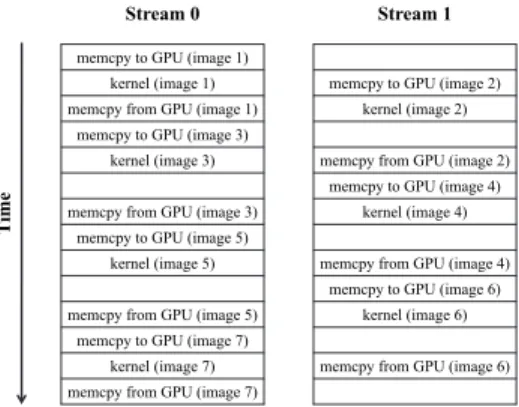
Fig. 4: Two Streams in one GPU.

Below we will see a method for achieving a kind of task-level parallelism in our GPU-based implementation, which is based on

CUDAstreams. Streams implement a task mechanism on the GPU,

which allows parallel execution of jobs. A CUDA stream represents a queue of GPU operations that get executed in the order they are added to the stream.

In this version of the benchmark, we use two different CUDA streams to perform the work. Figure 4, shows the timeline of the application execution when we are using those two independent streams and if we assume that the memory copies and the kernel executions take roughly the same time. Stream 0 will start with the first image by performing a memcpy to the GPU (which is loading the image) and then it will continue with the kernel execution, while stream 1 copies its input buffers to the GPU. After that stream 0 will copy its results to the host, while stream 1 will proceed with the kernel execution of the second image. The Figure 4 shows that the GPU can perform a kernel execution and memory copy at the same time, while the empty spaces represent the time that a stream waits to execute an operation that cannot overlap with an operation of another stream. While one stream is executing a memory copy, another stream will execute a kernel1.

In order to successfully perform the overlapping of the transfers and the GPU computations, we used pinned memory on the host.

Pinned memory, or page locked memory, is a special kind of

dynamically allocated memory, which has the property not to be paged out. This means that this memory chunk will never be swapped in the disk, in order the physical memory page to be given to another process.

Due to this fact, the use of pinned memory not only reduces the latency that the process spends for its memory to be swapped in, but also makes the transfers faster. This happens because the CUDA driver doesn’t need to copy this memory to a temporary page-locked buffer before giving control to the DMA controller to complete the transfer, but instead it uses the same buffer for this operation. For this reason, this optimization is known asZero-Copytransfer.

The drawback of the pinned memory, however, is that it is more expensive to be obtained from the operating system, since it is an expensive resource. In our case this is not a big problem, because the amount of pinned memory we require is small (120KB per image, so 480KB in total) and additionally the allocation cost is paid only once during the initialization phase, which is very short compared with the actual execution time.

1_{In fact, high-end systems can even execute two memory transfers at the}

same time, one from the GPU and one towards the GPU, therefore the actual overlapping in the system might be even more aggressive than the depicted one.

(5)

Ti

m

e

Device 0

Ti

m

e

memcpy to GPU (image 4) kernel (image 4) memcpy from GPU (image 4) Device 1

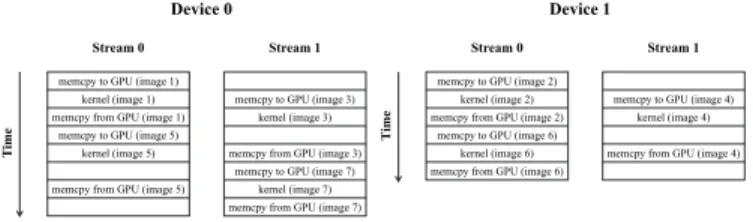
Fig. 5: Two Streams in each one of the two GPUs.

C. Using Two GPUs with MPI

In this version of the application we are taking advantage of multiple GPUs and CPUs that may exist in an architecture. A limitation of CUDA is that each thread can use a single GPU device. Therefore, in order to use a second GPU we are going to need a separate CPU context which will control it. In a multi-processor platform, as the one we used for the evaluation, the new CPU thread can run in parallel without any loss of performance.

In order to implement this scheme we used MPI to create two processes, each one coupled with a GPU device. For each of the devices we continue to use two streams as before.

In order to achieve the best performance we pin each process in the CPU that is closer to the GPU that it is controlling. Moreover, we allocate memory closer to that CPU, so that the memory transfers are more effective.

Figure 5 shows the timeline of the application execution for device 0 and device 1 respectively.

D. Improve CPU and GPU overlapping

Although asynchronous GPU operations provide a way of over-lapping CPU and GPU tasks, there is still a limiting factor. This factor – which in our case is the bottleneck of the system as we explain in the Evaluation Section – is the file I/O. Read and write operations of the input and output images respectively are expensive

blockingoperations. This means that when the CPU requests data to

be read from a file, the operating system blocks the process until the requested data are retrieved from the disk. When the data are ready, the operating system wakes up the process to continue its execution. However this operation can take millions of processor cycles, since the disk is several orders of magnitude slower than the CPU.

The same problem is encountered during file write operations, which is an even slower operation. Therefore, in order to increase the performance of our benchmark we need to attack this problem. Note that the blocking behavior of reading requests is not a problem in our design, since at some point we have to wait until the previous operation in the same stream is finished.

However, the blocking nature of write does create a problem, because the file read of the new image and the subsequent GPU operations are delayed until the image is written in the disk, because the process is unable to proceed. There are two solutions to this problem: one is the use ofasynchronous I/Ofor image writing or the elimination of the image writes completely.

The use of asynchronous I/O for image writing gives the opportu-nity to a process to continue immediately after an I/O request. The process associates a callback function which is going to be called at the completion of the request. This way, the file descriptor of the file can be closed after the completion of the write request.

In our implementation, after all the images are correctly processed, we wait until all the write requests are completed, and close the files

before exiting. As we discuss in the Evaluation Section, our program spends the majority of its time in this waiting phase.

An alternative solution that is common in previous works [12] is to skip completely the image writing. This depends on the particular application. For example, in an ADAS system typically the output doesn’t need to be written in a file (unless it is required for legal purposes) but instead to be projected on a display and inform the cruise system about the position of the detection for possible emergency breaking. These operations don’t have the cost of writing the output image and can give a significant boost on the performance of the system, as we see in the next Section.

VI. EXPERIMENTALEVALUATION

In this Section we present and analyze the results of our ADAS benchmark in a reference multi-CPU multi-GPU platform. All the experiments have been conducted on a Quad Core AMD with 2 Dual-Core AMD Opteron Processors 2222 3GHz, with 1MB cache. The host is equipped with two NVIDIA Tesla C2050 graphic cards. The classifier we used is provided together with the original appli-cation [14], and it was produced as a result of the training of the classifier with a specific set of images. The application has been tested with a set of 100 greyscale input images with resolution 640x480. We paid special attention to ensure that the output of the GPU implementations matches the output of the original CPU version. Our classifier contains 30 stages and we are using 30 different scales. The images have been selected from various well-established pedestrian datasets such as Caltech [7] and INRIA [5].

A. Evaluation Methodology

The baseline application has been designed to process a single frame per execution. However, since our GPU implementation is almost 2 orders of magnitude faster than the CPU implementation and returns almost instantaneously, there is significant possibility measurements to be affected by errors. Additionally, in this way CPU implementation is favored compared to GPU, because GPU has an additional overhead of the driver initialization and pinned memory allocations that are paid once. Finally, a pedestrian detection application should be designed to run repeatedly over video frames [1] (e.g. in a real automotive system).

For the above reasons we decided to modify the original application in order to process multiple images per run. The numbers of our experiments are averaged numbers of 1000 experiments using 100 different image inputs per execution.

B. Overall Application Performance

In this section we evaluate the performance of our benchmark implementation compared to the sequential optimized version of the open source application used as baseline.

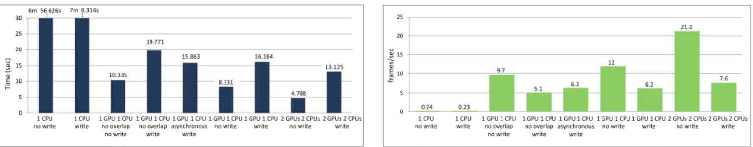
In Figure 6 we see the overall execution times of our benchmark for the various optimizations we have performed. There are two pairs of execution times that summarize the effectiveness of our imple-mentation. The first one is the comparison of our most optimized version, which features 2 CPUs and 2 GPUs, overlapping between CPU executions, GPU executions and GPU memory transfers and write of output image in the disk, with the most optimized CPU version of the baseline application that also writes the outcome in the disk. Our version is 32 times faster than the original application. Although this is a significant speedup over the original application, it is below the desired frame rate of 15 frames per second. In fact as shown in Figure 7, it achieves 7.6 frames per second compared to the baseline application, which achieves only 0.23 frames per second.

(6)

0 5 10 15 20 25 30 10.335 19.771 15.863 8.331 16.164 4.708 1 GPU 1 CPU no overlap no write 1 GPU 1 CPU no overlap write 1 GPU 1 CPU asynchronous write 1 GPU 1 CPU no write 1 GPU 1 CPU write 2 GPUs 2 CPUs no write 2 GPUs 2 CPUs write Time (sec) 1 CPU no write 1 CPU write 13.125 7m 8.314s 6m 56.626s … …

Fig. 6: Execution times of different versions of our benchmark for 100 images.

However this happens because the application is limited by the storage I/O capabilities of our system. If we take a look in the pair of the same implementation without the image writing to the disk, but instead we display it on the screen, our implementation achieves 21 frames per second while the CPU just 0.24 frames per second. This shows that obviously the disk writing speed is the bottleneck in our implementation, since the elimination of image writing provides a speedup of 2.7 times over the writing version. On the other hand, this is not the case for the CPU, as it only gives a 2% improvement over the corresponding CPU implementation, showing clearly that it is CPU bound.

This modification in the application is common in previous works [12] and it is acceptable in an automotive system, because it is diskless and there is no benefit of storing the processed frame. On the other hand, it is useful to display the detected object on a screen and provide information about the detection to the cruise system, which will decide whether there is a need for emergency break or warning the driver.

Therefore our implementation has been able to achieve a process-ing frame rate well above the requirement of 15 frames per second, achieving an overall speed-up of 88.5×over the CPU implementation with the same feature.

Next we are going to discuss the performance of different parts of our implementation as well as the effect of the various optimizations we performed.

C. Integral Image Performance

In Figure 8a, we compare the execution times of the integral image and the DotSquare image in CPU (blue) and the GPU (red). The integral image computation in the GPU is 49.6 times faster than in CPU, while the speedup of the DotSquare image is 416.6. Here, it is important to note that we used the execution time of the first integral image invocation, for the reason we explain later on.

In Figure 8b, we have a closer look of the GPU break down of the first phase of the application. Surprisingly, the second execution of the integral image is a lot faster (approximately 7.5 times faster) than the first one. This happens, because the input of the second integral image was the DotSquare and it was being kept in the large L2 cache of the GPU.

D. Effect of CPU-GPU overlapping

As explained in the previous section, the first overlapping optimiza-tion we performed is the overlapping of CPU and GPU operaoptimiza-tions. This is because the GPU operations are no longer synchronous and therefore gives us a first degree of overlapping. When combined with overlapping of GPU tasks as transfers and GPU kernel execution, it can provide significant speedups.

0 5 10 15 20 25 9.7 5.1 6.3 12 6.2 21.2 7.6 1 GPU 1 CPU no overlap no write 1 GPU 1 CPU no overlap write fr ames/ sec 2 GPUs 2 CPUs write 1 GPU 1 CPU write 1 GPU 1 CPU no write 1 CPU no write 1 CPU write 0.23 0.24 1 GPU 1 CPU asynchronous write 2 GPUs 2 CPUs no write

Fig. 7: Frames per second achieved for each version of our bench-mark, when running with 100 images.

0,00 0,50 1,00 1,50 2,00 2,50 3,00 3,50 4,00 4,50

Integral Image Dot Square Image CPU GPU (ms) 4.166 0.01 4.465 0.09 (a) 0,900 0,920 0,940 0,960 0,980 1,000 1,020 1,040 1,060 1,080 GPU Integral Image 2 Dot Square Image Integral Image 1 Data Transfer

(ms)

(b)

Fig. 8: (a) Integral image and DotSquare image execution time in CPU and GPU (b) Detailed view of the benchmark’s first phase execution time in GPU.

In order to isolate the effect of this optimization, we evaluate it only in the single CPU and GPU version. For the version of the application that writes the output image to the disk, this optimization gives an improvement of 22%. On the other hand, for the version that the image is displayed, this speedup is increased to 24%.

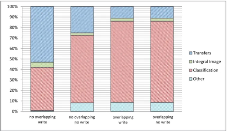
Figure 9 illustrates the contribution of transfers in the total execu-tion time with and without overlapping. When no overlapping takes place, transfers occupy 53% when the processed image is written to the disk and 25% when the image is displayed on the screen. This percentage is reduced to 11% in both scenarios when overlapping is performed.

E. Effect of asynchronous file I/O

As explained earlier in this Section, the bottleneck of our bench-mark is the storage subsystem. Although in an ADAS system it seems that there is no reason for the output image to be written in the disk, someone can argue that the last processed frames must be stored (similar to an aircraft’s black box), due to legal obligations or because they are demanded by insurance companies in case of an accident. For this reason, we implemented an optimization to mitigate the performance impact of the disk operations.

As described in the previous Section, we used asynchronous file I/O for the write requests of the application. This enables the application not to be blocked during the expensive image writes but to continue doing useful work, such as reading the next frame and scheduling GPU tasks.

(7)

0% 10% 20% 30% 40% 50% 60% 70% 80% 90% 100% Transfers Integral Image Classification Other no overlapping write no overlapping no write overlapping write overlapping no write

Fig. 9: Execution time break-down for our different benchmark versions.

As we can see from the Figure 6, this gives an improvement of 2% in the overall execution time. However, this number is misleading and doesn’t show the absolute advantage of this optimization, since this number corresponds to the execution time of the entire application. If we have a closer look, we can see that our application finishes the processing of the 100 images in almost the same time as when write is suppressed (8.5 sec instead of 8.3 sec) and the rest of the time is spent on waiting for all the asynchronous requests to be completed, in order to close their files. This means that we achieve the same processing frame ratio (throughput), but the application spends 53% of its time doing nothing but waiting for the asynchronous requests to be completed.

Something about the effectiveness of this optimization that is worth to mention, is that it achieves full utilization of our reference platform, when the version of 2 CPUs and 2 GPUs with overlapping is used. This happens because each of the 2 CPU processes are constantly able to issue work to their respective GPUs, so 2 CPUs and 2 GPUs are kept busy. Moreover, the DMA controllers are working in parallel to transfer data between the two CPUs and the two devices, while the other 2 CPUs of our system are free to handle the asynchronous I/O requests issued by the other CPUs.

To sum up, we have shown that our system has managed to achieve full utilization of our hardware platform, even though it is limited by the file operations. Note that this implication would be less harmful for the performance of our application if instead of individual images, the program would read/write video frames. This would reduce the I/O bandwidth and increase the I/O throughput, since in this case the frames would be stored in a compressed form and in consecutive file blocks. The benefit comes from the fact that usually sequential reads perform better in many systems, compared to random reads. The same case is for writes, although they are much slower than reads in both cases.

VII. RELATEDWORK

There is a wide collection of object recognition algorithms and more concretely algorithms specialized on face-detection / pedestrian detection [8] in the computer vision and machine learning literature. An extensive enumeration of all the proposed algorithms is out of the scope of this paper, however we try in this section to provide the most influential work in this domain and refer works similar to ours. The Viola-Jones method [16][17] is the most influential work in face detection, because it introduced the AdaBoost training algorithm,

and the cascade classifier, which consists of many weak classifiers organized in stages, in order to create a strong classifier. In its era this method provided the highest accuracy with the faster execution time. The authors reported an achieved processing rate of 15 frames per second (fps) on 384x288 images. All the later proposed algorithms have the same structure, based on a cascade classifier but use different weak classifiers. Moreover, all these algorithms use a sliding window to perform detections.

Dalal and Triggs [5] introduce the concept of grid of Histogram of Oriented Gradient (HOG) that outperform Haar features in detection accuracy and introduce the INRIA pedestrian detection dataset.

Doll´ar et al. [6] propose a modification in the Viola-Jones algo-rithm, which can speed up the CPU implementation an order of magnitude. Although this gives significant performance benefit, their reported image processing rate for the same image size we use, is 5 frames per second.

Zhang and Nevatia [18] propose a GPU implementation of a classifier based on Histogram of Oriented Gradient (HOG) instead of Haar features. Moreover, instead of integral images, the algorithm uses a precomputation analogous to integral image, which is less computational intensive. In this work, only one GPU is used, without overlapping computation and transfers. Moreover the only GPU related optimization used is the load of input data to texture memory, to take advantage of its interpolation capabilities.

Doll´ar et al. [7] introduce the Caltech Dataset and compare different pedestrian detection algorithms running on the same CPU hardware. The Viola-Jones method was the second fastest one (7 seconds/frame) while the other ones were between 2-30 times slower. However, this difference in performance comes at the cost of lower detection rate compared to algorithms based on HOG features.

Oro et al. [12] implement a system based on Viola-Jones which uses 1080p video frames. They report processing rates of 35 fps, without however considering the transfer costs to and from GPU. Moreover, their work is focused on face-detection, which requires weaker classifiers compared to the human body detection.

Hefenbrock et al. [4] is the only work in the literature that uses multiple GPUs. This work is again focused on face detection, and therefore uses a simpler classifier cascade with 22 stages, compared to our 30-stage classifier. In addition, the image is scanned for nearly 40% less scales (18 instead of 30 in our system). Despite that their configuration has lower computational requirements, and that they utilize 4 GPUs with similar computational power to ours, they achieve a processing rate of 15.2 frames per second. Our implementation has superior performance with similar hardware (same generation CPU and GPUs), but with half the number of graphics devices under more complex detection scenarios. Although their various kernel implementations are highly optimized, we believe that this important performance difference comes from their scheduling of CPU and GPU tasks, which doesn’t allow overlapping between the execution of CPU, GPU and DMA controllers. Finally, the evaluation of this paper is performed with only 9 images. This means that the total execution time of their executions is less than a second, which is subject to significant measurement errors.

Note that independently from performance, none of the related GPU implementations [4][12][18] is available in open source, there-fore cannot be used as benchmark for the evaluation of ADAS platforms, which is our primary goal. In addition, all these mentioned works concentrate only on algorithmic or kernel optimizations, ignor-ing other aspects which we consider and we show that can be the platform bottlenecks, such as various tasks overlapping and I/O.

(8)

VIII. CONCLUSIONS ANDFUTUREWORK

In this paper we presented an open-source implementation of a hybrid multi-CPU and multi-GPU ADAS benchmark. Our baseline application, is based on a sequential open source implementation of the Viola-Jones detection algorithm for pedestrian detection. We explained the design and optimization details of our multi-CPU and multi-GPU implementation benchmark. Our evaluation on a reference platform is 88.5× times faster than an optimized CPU version, achieving 21 frames per second, being comparable with non-public ADAS systems with similar specifications.

We hope that our implementation will be useful to both industry and academia to assess the capabilities of future architectures for au-tomotive ADAS systems. Our plans for future work include creating an OpenCL version of our benchmark in order to cover more potential platforms. Finally, we encourage other researchers from academia and industry (when is possible, due to IP) to provide more open source ADAS applications, so that the automotive community can be developed faster towards automated driving.

ACKNOWLEDGMENTS

This work has been supported by the Spanish Ministry of Science and Innovation under grant TIN2015-65316P, the HiPEAC Network of Excellence and a Microsoft sponsored ACM SRC. The first two authors acknowledge Dr. Petrisor for her assistance in understanding and using the sequential version of the benchmark and dedicate this article to the memory of the late beloved advisor prof. Nacho Navarro, without whom this work would not have been possible.

REFERENCES

[1] Rosa M. Badia, Yoav Etsion, Sylvain Girbal, Antoni Portero, and Mikel Lujan. D2.1 report on the reference set of applications chosen, and initial characterization of the applications. Public deliverable, TERAFLUX Project (FP7/2010-2014 grant agreement no 249013), 2010.

[2] Rosa M. Badia, Yoav Etsion, Sylvain Girbal, Antoni Portero, and Mikel

Lujan. D2.2 final report on the characterization and modeling of

the reference applications. Public deliverable, TERAFLUX Project

(FP7/2010-2014 grant agreement no 249013), 2011.

[3] Rosa M. Badia, Tomasz Patejko, Yoav Etsion, Sylvain Girbal, Antoni Portero, and Mikel Lujan. D2.3 initial report on applications already ported to the new dataflow based programming model. Public deliver-able, TERAFLUX Project (FP7/2010-2014 grant no 249013), 2012. [4] D. Hefenbrock et al. Accelerating Viola-Jones Face Detection to

FPGA-Level Using GPUs. InInternational Symposium on Field-Programmable

Custom Computing Machines (FCCM), 2010.

[5] N. Dalal and B. Triggs. Histograms of oriented gradients for human

detection. InIEEE Computer Society Conference on Computer Vision

and Pattern Recognition (CVPR), 2005.

[6] P. Doll´ar, S. Belongie, and P. Perona. The Fastest Pedestrian Detector

in the West. InBritish Machine Vision Conference (BMVC), 2010.

[7] P. Doll´ar, C. Wojek, B. Schiele, and P. Perona. Pedestrian detection: A

benchmark. InIEEE Computer Society Conference on Computer Vision

and Pattern Recognition (CVPR), 2009.

[8] P. Doll´ar, C. Wojek, B. Schiele, and P. Perona. Pedestrian Detection:

An Evaluation of the State of the Art. IEEE Transactions on Pattern

Analysis and Machine Intelligence, 34(4):743–761, 2012.

[9] International Organization for Standardization, 2009. ISO/DIS 26262.

Road Vehicles – Functional Safety.

[10] M. Sierhuis, Nissan. Socially Acceptable AI-based City Driving.keynote

at International Conference On Computer Aided Design (ICCAD), 2016.

[11] OpenCV. OpenCV Library: Open Source Computer Vision Library,

1999. http://opencv.willowgarage.com.

[12] D. Oro, C. Fernandez, J.R. Saeta, X. Martorell, and J. Hernando.

Real-time GPU-based face detection in HD video sequences. InInternational

Conference on Computer Vision Workshops (ICCVW), 2011.

[13] S. Burton, Bosch. Engineering Dependable Platforms For Automated

Driving. Invited Talk at Automotive Day, Design, Automation and Test

in Europe (DATE), 2017.

[14] T. Petrisor, Thales Group. Viola-Jones Case Study at TERAFLUX public svn, 2010.

[15] Matina Maria Trompouki. Multi-CPU/GPU Pedestrian Detection.

http://github.com/mtrompouki/pedestrian detection.

[16] Paul Viola and Michael Jones. Rapid Object Detection using a Boosted

Cascade of Simple Features. InComputer Vision and Pattern

Recogni-tion (CVPR), 2001.

[17] Paul A. Viola and Michael J. Jones. Robust real-time face detection.

International Journal of Computer Vision, 57(2):137–154, 2004.

[18] Li Zhang and R. Nevatia. Efficient scan-window based object detection

using GPGPU. InComputer Vision and Pattern Recognition Workshops