Tasmanian School of Business and Economics
University of Tasmania
Discussion Paper Series N 2018-02
Analysis of shock transmissions to a small
open emerging economy using a SVARMA
model
Mala Raghavan
University of Tasmania, Australia
George Athanasopoulos
Monash University, Australia
Analysis of shock transmissions to a small open
emerging economy using a SVARMA model
Mala Raghavana,b∗ George Athanasopoulosc
a
Tasmanian School of Business and Economics, University of Tasmania, Australia b
Centre for Applied Macroeconomic Analysis, Australian National University, Australia c
Department of Econometrics and Business Statistics, Monash University, Australia
Abstract
Using a parsimonious structural vector autoregressive moving average (SVARMA) model, we analyse the transmission of foreign and domestic shocks to a small open emerging economy under different policy regimes. Narrower confidence bands around the SVARMA responses compared to the SVAR responses, advocate the suitability of this framework for analysing the propagation of economic shocks over time. Malaysia is an interesting small open economy that has experienced an ongoing process of eco-nomic transition and development. The Malaysian government imposed exchange rate and capital control measures following the 1997 Asian financial crisis. Historical and variance decompositions highlight Malaysia’s high exposure to foreign shocks. The ef-fects of these shocks change over time under different policy regimes. During the pegged exchange rate period, Malaysian monetary policymakers experienced some breathing space to focus on maintaining price and output stability. In the post-pegged period, Malaysia’s exposure to foreign shocks increased and in recent times are largely driven by world commodity price and global activity shocks.
Keywords: SVARMA models, Open Economy Macroeconomics, ASEAN, Shock trans-missions.
JEL classification numbers: C32, F41, F62, E52
∗
Corresponding author: Mala Raghavan, Tasmanian School of Business and Economics, University of
Tasmania, Private Bag 85, Hobart, TAS 7001, Australia. E-mail: [email protected]; Tel no: +61362262895
1
Introduction
Since the seminal paper by Sims (1980), structural vector autoregressive models (SVARs) have dominated empirical macroeconomics. Despite their popularity for modelling ad-vanced economies, the use of SVARs for emerging economies has been challenging. Such economies are usually plagued by frequent structural breaks and policy changes, due to the ongoing process of economic transition and development Hence, compiling adequate data sets for policy analysis for such economies is problematic. Furthermore, a small dimensional SVAR model would require a long lag structure to capture the empirical dynamics of the data in order to produce plausible results that are consistent with economic theory and stylized facts (Kapetanios et al., 2007). Such issues cause serious impediments to empirical research, particularly for small open emerging economies. An alternative would be the use of a parsimonious structural vector autoregressive moving average (SVARMA). Dufour and Pelletier (2002, 2011) and Raghavan et al. (2016) illustrate the VARMA representation to be more appropriate for macroeconomic modelling to the VAR counterpart.
In this paper, we build a SVARMA model to examine the transmission of foreign and domestic shocks to a small open emerging economy - Malaysia. In mid-1997, along with its Southeast East Asian neighbours, Malaysia was affected by the Asian financial crisis which caused a huge financial and economic turmoil in these region. In September 1998, the Malaysian government took the controversial decision of implementing exchange rate and selective capital control measures to stabilize the depreciating exchange rate and to mitigate the short term capital outflows. Since early 2000, there was a continuous liberalisation of foreign exchange administration rules as Malaysia gradually lifted policies implemented in 1998. In mid-2005, Malaysia reverted back to managed float exchange rate regime. In view of the change in the financial environment and the choice of policy regimes, the objectives of this paper are to: (i) build a Malaysian SVARMA model and establish the necessary identification conditions to uncover the independent foreign and domestic shocks; (ii) assess whether a small dimensional Malaysian SVARMA model compared to SVAR model produces impulse responses that are consistent with economic theory and stylized facts, and (iii) examine the drivers of foreign and domestic shocks over time, under the different policy regimes experienced by Malaysia.
difficulties in identifying and estimating unique VARMA representations.1 Therefore, ap-plied researchers tend to approximate a VARMA process by a VAR model of order that is much higher than that selected by AIC or BIC, to describe the system adequately and to obtain reliable impulse responses (Kapetanios et al., 2007). However, for open emerging economies the available sample sizes are inadequate to accommodate a sufficiently long lag structure. This leads to poor approximations of the model, loss of information and the unreliability of impulse responses. Athanasopoulos and Vahid (2008a) propose a canonical VARMA model by extending the work of Tiao and Tsay (1989). They establish sufficient conditions for uniquely identifying the model so that all parameters can be identified and estimated simultaneously using full information maximum likelihood (FIML).
We apply the methodology of Athanasopoulos and Vahid (2008a) to build a model for Malaysia within the VARMA framework. To identify the contemporaneous structure of the model, we employ identification restrictions similar to Raghavan et al. (2012). These are broadly consistent with the preferred theory and stylized facts. Using monthly data of seven variables from January 1985 to December 2015, we investigate the dynamic responses of the Malaysian economy to domestic and foreign shocks. The global activity index, the world commodity price index and the shadow Federal funds rates represent the foreign variables while the Malaysian industrial production index, consumer price inflation, overnight inter-bank rates and real effective exchange rate represent the domestic variables. The choice of foreign business cycle variables is different to those commonly used in the literature. We use the global activity index developed by Kilian (2009) to capture the fluctuations of the global output instead of the commonly used US production index. Since December 2008, the Federal funds rate has been close to zero. To quantify the stance of the US unconventional monetary policy in the “zero lower bound” environment, instead of the commonly used Federal funds rate we use the shadow rate developed by Wu and Xia (2016) as the US monetary policy variable.
The orthogonal foreign and domestic shocks identified through the SVARMA models are used to evaluate the impulse responses and historical decomposition of the domestic variables to these shocks. Similarly to Raghavan et al. (2016), the SVARMA models pro-duce reliable dynamic impulse responses, as predicted by theory and stylized facts; in this 1See for example Hannan and Deistler (1988); Tiao and Tsay (1989); Reinsel (1997); L¨utkepohl (2005).
case for a small open emerging economy.2 The confidence bands around the SVARMA responses appear to be narrower than those around SVAR responses, indicating more pre-cise impulse response functions. The historical decompositions highlight Malaysia’s high exposure to foreign shocks and the effects of these shocks are found to change over time under different policy regimes. During the pegged exchange rate regime, foreign shocks contributed negatively, particularly on interest rates and the real exchange rate, while in the years since 2006 foreign shocks contributed positively to all four domestic variables.
In view of the change in Malaysian policy regimes, we divide the period of study into: a pre-crisis period (1985:1 to 1997:12), a pegged exchange rate period (1998:9 to 2005:6) and a post-pegged exchange rate period (2006:1 to 2015:12). The three sub-periods are considered primarily to assess the impact of the changes in the exchange rate regime on the Malaysian shock transmission mechanism; Malaysia adopted a managed float exchange rate regime during the pre-crisis and the post-pegged periods. The foreign and domestic shocks identified for each sub-period are used to evaluate the forecast error variance decomposition of the domestic variables to these shocks. The variance decomposition shows that in the pre-crisis period, both foreign and domestic shocks are important sources of fluctuations for output and inflation. Overall, during this period the exchange rate played an important role in influencing the domestic variables. During the pegged exchange rate period, the exchange rate shock has subdued effects on all domestic variables while the US monetary shocks appear to be an important source of fluctuation followed by the real global activity shock. During this period, Malaysian monetary policymakers enjoyed some breathing space focusing on maintaining price and output stabilities. The post-pegged period coincides with the increase in world commodity prices that are connected with a surge in the demand for commodities from emerging economies. As expected, during this period, the world commodity price shock is an important driver of the Malaysian economy.
The empirical results provide some valuable insights into the transmissions of shocks under different policy regimes experienced by Malaysia. Further, the results are consistent with the recent ADB (2017) report, which states that the ASEAN economies are vulnerable to global activities, commodity prices and US monetary policy surprises. The identified SVARMA model, thus could assist in the modelling of the business cycle framework of 2In Raghavan et al. (2016), the SVARMA framework was applied to model and assess the monetary policy framework of an advanced small open economy - Canada.
similar open emerging economies, especially the economies that are not currently studies due to limited data availability.
The paper is organized as follows: Section 2 briefly discusses the Malaysian economy. Section 3 describes the VARMA methodology and its benefits. Section 4 illustrates the identification of the Malaysian SVARMA model and the choice of variables. Section 5 reports and discusses the empirical findings and Section 6 concludes this paper.
2
The Evolution of the Malaysian Economy
The Malaysian economy has evolved in line with the liberalization and globalization pro-cesses and witnesses widespread changes in the conduct of monetary policy and the choice of monetary policy regime (see for example Tseng and Corker, 1991; Dekle and Pradhan, 1997; Athukorala, 2001; McCauley, 2006; Umezaki, 2006).3 In the mid-1980s, while main-taining a managed float exchange rate system, the conduct of monetary policy by Bank Negara Malaysia (BNM), not only depended on inflation and real output but also on foreign monetary policy (see Cheong, 2004; Umezaki, 2006, for details). BNM’s monetary strategy was to focus on monetary targeting as it was found to be closely linked to inflation.
To maintain it’s monetary policy objectives of price and exchange rate stabilities and output growth sustainability, BNM influenced the day-to-day volume of liquidity in the money market to ensure that the supply of liquidity is sufficient to meet the economy’s demand for money. Subsequent developments in the economy and the globalization of financial markets in the early 1990s however weakened the relationship between monetary aggregates and the target variables of income and prices (see for example Tseng and Corker, 1991; Dekle and Pradhan, 1997). Around this time, the globalization process also caused notable shifts in the financing pattern of the economy, that is moving from an interest-inelastic market (government securities market) to a more interest rate sensitive market (bank credit and capital market). As investors became more interest rate sensitive, the monetary policy framework based on interest rate targeting was seen as an appropriate measure to promote stability in the financial system and to achieve the monetary policy objectives. As a result, in the mid-1990s, BNM shifted towards an interest rate targeting framework.
3Monetary policy regimes are characterized by the degree of autonomy in the conduct of monetary policy, the choice of exchange rate regime and the degree of international capital mobility.
The globalization process came with a cost to Malaysia as the economy not only was vul-nerable to domestic shocks but was also largely exposed to foreign shocks. The mid-1997 East Asian financial crisis had substantial impact, mainly putting significant downward pressure on the Malaysian Ringgit. The Ringgit declined from about RM2.5 per US dollar to RM4.0 per US dollar. As can be see in Figure 7 in the Appendix, the depreciation of the Ringgit caused a temporary rise in inflation to levels well above the long-term av-erages.4 The volatile short-term capital flows and the excessive volatility of the Ringgit made it impossible for BNM to influence interest rates based on domestic considerations. In September 1998, Malaysia imposed exchange rate and selective capital control measures to stabilize the depreciating exchange rate. The Ringgit was fixed at RM3.80 per US dollar, while the short-term capital flows were restricted. These measures were needed to provide BNM the required breathing space to embark on expansionary monetary policy to overcome the contraction of the economy.
Prior to the 1997 crisis, BNM paid systematic attention to expected inflation while at the same time maintained a managed float exchange rate system. However, the conduct of monetary policy was rather flexible due to its vulnerability to both domestic and foreign shocks (see Cheong, 2004; Umezaki, 2007). In the pegged period, the exchange control measure gave BNM some degree of monetary autonomy to influence the domestic interest rates without having to pay so much attention on managing the Ringgit exchange rate. Since then, the focus of monetary policy had been to manage the liquidity level in the economy in order to maintain the interest rate at a level that is sufficiently low to promote economic growth. The pegged exchange rate is expected to provide stability and certainty to facilitate and improve trades and investments. In this regard, the policy continues to be directed at sustaining, and where necessary strengthening the economic fundamentals to support the sustainability of the exchange rate. In 2005, Malaysia scrapped the Ringgit’s peg to the US dollar and again gradually adopted a managed float exchange rate system with the focus on targeting the effective exchange rate. For more details on the evolution of the Malaysian monetary policy since the 1997 financial crisis can be found in Athukorala (2001); Azali (2003); Cheong (2004); Ooi (2008); Singh et al. (2008) and Shimada and Yang (2010).
4However, one should note that the rise in inflation was still mild compared to that during the supply driven oil shocks around 1980 and demand driven oil shocks around 2008.
Malaysia continued to post solid growth rates, averaging around 5.5% per year from 2000-2008.5 Though the Malaysian economy was hit by the Global Financial Crisis (GFC) in 2009 it recovered quickly, posting growth rates averaging 5.7% from 2010. The im-plementation of appropriate policy measures such as developing a framework to deal with foreign currency helped improve the soundness of the Malaysian banking system and macro-prudential responses compared to the Asian crisis period. Hence, Malaysia showed consid-erable resilience during the 2008/09 global financial and economic crisis period. However, the surge in capital inflows during the 2009/2010 reminded Malaysian monetary policy makers of the inherent risks if these are channeled into the capital and real estate markets. The large exposure to foreign funds can make banking systems vulnerable, while exposing the economy to the vagaries of external shocks (Tng and Kwek, 2015).
The above mentioned discussion highlights that open emerging economies like Malaysia are subject to large macroeconomic volatilities compared to developed economies due to fre-quent policy changes. This makes macroeconomic modeling a challenging process. Paying attention to implementing parsimonious well thought out models is essential for overcoming the issues concerning the compilation of adequate data for such economies.
3
VARMA models
It is essential for policy makers to make an accurate assessment of the timing and the effects of shocks on economic activities and prices. Although VARs provide a useful tool for evaluating the effect of foreign and domestic shocks, there are ample warnings in the literature about their limitations both on theoretical and practical grounds. In what follows, we first discuss some of the justifications provided in the literature for the use of VARMA models over VARs and subsequently provide a brief discussion of the Athanasopoulos and Vahid (2008a) methodology for identifying and estimating a VARMA model.
3.1 VARMA versus VAR
There are numerous theoretical and practical justifications and recommendations to em-ploy VARMA models over VARs (see for example Zellner and Palm, 1974; Granger and Morris, 1976; Wallis, 1977; Maravall, 1993; L¨utkepohl, 2005). Economic and financial time series involve for example seasonal adjustment, de-trending, temporal and
contemporane-5
ous aggregation. Such time series include moving average dynamics even if one assumes its constituents being generated by a VAR. A subset of variables coming from a multivariate VAR process should be modelled using a VARMA model rather than a VAR (see Fry and Pagan, 2005). Cooley and Dwyer (1998) claim that the basic real business cycle mod-els follow VARMA processes, while Fern´andez-Villaverde et al. (2007) demonstrate that linearized dynamic stochastic general equilibrium models in general imply a finite order VARMA structure.
The main purpose of business cycle analysis is to generate impulse response functions of domestic variables to various shocks. These impulse responses are derived by appealing to Wold’s decomposition theorem. In a multivariate Wold representation, a long order VAR can be transformed into an infinite order vector moving average (VMA) process of its innovations. A finite order VARMA model would provide a better approximation to the Wold representation than a long finite order VAR model. Hence, VARMA models are expected to produce more reliable impulse responses than the VAR models. Using the US and Canada as a case studies,Dufour and Pelletier (2011) and Raghavan et al. (2016) respectively illustrate that the parsimonious SVARMA models provide more precise impulse response functions compared to SVARs. In an extensive empirical study, Athanasopoulos and Vahid (2008b) also show that VARMA models forecast macroeconomic variables more accurately than VARs. The preceding discussion suggests that the SVARMA framework will be a more attractive alternative than the existing SVAR counterparts for macroeconomic modelling. In this paper we provide further empirical evidence supporting this claim by comparing the two classes of models for modelling a small open economy.
3.2 Identification of a VARMA model
A K dimensional VARMA(p, q) process can be written as
Xt=A1Xt−1+. . .+ApXt−p+υt−M1υt−1−. . .−Mqυt−q, (1)
where Aj represent the autoregressive coefficients while Mi represent the moving average
(MA) coefficients. To identify and estimate (1) we use the Athanasopoulos and Vahid (2008a) extension of the Tiao and Tsay (1989) scalar component model (SCM) methodology. The aim of identifying scalar components is to examine whether there are any simplifying embedded structures underlying this process that can provide a parsimonious VARMA
structure. A detailed exposition of the methodology can found in Appendix A. The VARMA(p, q) in (1) can be written as
A(L)Xt=M(L)υt, (2)
whereA(L) =A0−A1L−A2L2−. . .−ApLpandM(L) =M0−M1L−M2L2−. . .−MqLq.
The effects of foreign and domestic shocks are analysed from impulse response functions which are derived from pure vector moving average representations (VMA) of the model. The VMA representation of (2) is given by
Xt=Φ(L)υt=υt+ ∞ X i=1 Φiυt−i (3) where Φi =Mi+ i X j=1 AjΦi−j
and Φ0 = Ik, Aj = 0 for j > p and Mi = 0 for i > q while υt is a (K×1) multivariate
white noise error process with the following properties of E(υt) = 0 andE(υtυ0t) =Ωυ.
However, the VMA processes in (3) does not allow us to attribute the response of a certain variable to an economically interpretable shock.6 One way to circumvent this problem is to transform these exogenous shocks into a new set of orthogonal shocks, with each element independent of one another. SVARMA and SVAR models use economic theory to identify the contemporaneous relationships between variables. We discuss this in detail in Section 4. The relationship between the reduced form VARMA disturbances (υt) and
the orthogonal shocks vt is
B0υt=vt, (4)
where B0 is an invertible square matrix, E(vt) = 0, E(vtv0t) = Σv and Σv is a diagonal matrix. B0 is normalized across the main diagonal, so that each equation in the system
has a designated dependent variable. The innovations of the structural model are related to the reduced form innovations by Συ =B−01Σv(B−01)
0. The impulse responses from the
SVARMA are obtained from
Xt=B−01vt+ ∞
X
i=1
ΦiB−01vt−i. (5)
Historical decomposition of a variable utilizes a representation of any variable in terms of the product of its impulse responses with estimates of the structural shocks. It allows
6
This is because υt is the combination of all fundamental economic shocks rather than featuring a
one to assess the contribution of each shock to the variable over time. The structural VMA representation of (5) is given by Xt= ∞ X i=0 Θivt−i (6)
whereΘi =ΦiB−01 and the historical decompositions can be derived by simply recognizing
that the VARMA form allows for any variable to be written as a weighted sum of previous shocks plus the effects of an initial condition, that is
Xt= initial conditions + t
X
i=0
Θivt−i (7)
and the contribution of thekth structural shock to thejth variable can be represented as
x(jtk) = initial conditions +
t
X
i=0
θjk,iνk,t−i (8)
Ideally plotting the x(jtk) for k = 1,2, ..., K, throughout the sample period, we could interpret and analyze the relative contributions of the different structural shocks to the
jth variable. Impulse response functions, historical decomposition and variance decom-postiion are derived and estimated to assess the persistence and dynamic effects of various macroeconomic shocks on policy and non-policy related variables.
4
Identifying a Malaysian SVARMA model
In this section, we apply the VARMA methodology to model the Malaysian business cycle. In addition to identifying and estimating a VARMA model as described in Section (3.2), we also discuss issues concerning foreign block exogeneity restrictions and the identification of the contemporaneous structure. The sample period of this study is from January 1985 to December 2015. It covers the post liberalization period in Malaysia and includes the mid-1997 East Asian financial crisis and the 2008 global financial crisis. To assess the impact of capital and exchange control measures on shock transmissions in the Malaysian economy, the period under study is divided into three sub-periods as described in Table 1.
Table 1: Breakdown of the period of study.
Description Period
Full period 1985:1–2015:12
Pre-crisis period 1985:1–1997:12
Pegged exchange rate period 1998:9–2005:6 Post-pegged exchange rate period 2006:1–2015:12
4.1 Choice of variables
We use monthly observations of seven variables which include both foreign and domestic variables to model the Malaysian economy. The three foreign variables are the real global activity index (GAI), world commodity price index (COM) and the shadow Federal funds rates (RUS). The GAI is used as a proxy for world output instead of the US industrial production index. It is the dry cargo shipping rate index developed by Kilian (2009) to capture the fluctuations of the global demand for industrial commodities.7 The COM is included to account for inflation expectations, mainly to capture the non-policy induced changes in inflationary pressure to which the central bank may react when setting monetary policy.8 Instead of using the Federal funds rate, we use the shadow rate (RUS) developed by Wu and Xia (2016) as a proxy of foreign monetary policy.9 Since December 2008, the Federal funds rate has been close to zero and to quantify the stance of the US unconventional monetary policy in the “zero lower bound” environment, it is more appropriate to use the shadow rate as the US monetary policy variable (see Wu and Xia, 2016; Krippner, 2013, for details.).
The remaining four domestic variables describe the Malaysian economy. The Malaysian industrial production index (IP) and the consumer price inflation (INF) are taken as the target variables of monetary policy, known as non-policy variables. INF is calculated by taking the annual change in the log of the consumer price index. The overnight inter-bank rate (IBR) represents the policy variable. In many studies on Malaysian monetary policy, the overnight interbank rate was selected as the instrument of monetary policy.10 The exchange rate is the information market variable. Considering the US dollar peg of the Malaysian Ringgit during the period of study, we employ the real trade-weighted index (TWI) instead of the bilateral US dollar exchange rate. The TWI is believed to capture more comprehensively the movements in the exchange rate that may have inflationary consequences in the Malaysian economy. These four domestic variables are also the standard set of variables used in the macroeconomic literature to represent small open economy 7For a detailed explanation on the construction and the interpretation of this index, please refer to Kilian (2009).
8Though Malaysia is an oil producing economy, it is highly trade intensive and energy intensive in its production, making it vulnerable to world commodity price changes (Downes, 2007; Raghavan et al., 2012). 9It is common in the monetary literature of small open economies to use the RUS as a proxy of foreign monetary policy (see for example Kim and Roubini, 2000; Dungey and Pagan, 2009; Raghavan et al., 2012).
10
business cycle models (see for example Kim and Roubini, 2000). Hence the vector of variables is represented as
Xt= [GAIt,COMt,RUSt,IPt,INFt,IBRt,TWIt]0
INF, RUS and IBR are expressed in percentages while GAI, COM, IP and TWI are sea-sonally adjusted and in logarithms.
Augmented Dickey Fuller and Philips-Perron unit root tests show that GAI, COM, RUS, IP and TWI are I(1) series while INF and IBR are I(0). Trace tests and maximum eigenvalue tests failed to clearly indicate whether cointegrating relationship exist amongst the I(1) variables. Given the mixed I(1) and I(0) nature of the data, VAR or VARMA models with variables in first differences will lead to loss of information in the long run relationships.11 Since the objective of this study is to assess the interrelationships among the variables and to correctly identify the effects of foreign and domestic shocks, with the exception of RUS, all other I(1) variables are de-trended using a linear trend.
4.2 Foreign block exogeneity restrictions
Shocks to small open economies have very little impact on the rest of the world. Therefore it is proper to treat the foreign variables as exogenous to Malaysian economic variables. To capture the foreign block exogeneity phenomenon, the variables are divided into foreign and domestic blocks as follows:
Xt= (X1,t,X2,t)0 (9)
where X1,t = (GAIt,COMt,RUSt)0 and X2,t = (IPt,INFt,IBRt,TWIt)0. The AR and MA
lag operators in a VARMA model as in equation (2) can be represented as follows:
A(L) = A11(L) 0 A21(L) A22(L) and M(L) = M11(L) 0 M21(L) M22(L) (10) It is assumed the foreign variables in the Malaysian VARMA system are predetermined and the domestic variables do not Granger cause the foreign variables. Hence, block exogeneity is imposed by excluding all domestic variables from entering the foreign block of equations
11
The impulse response functions generated from VECM models tend to imply that the impact of shocks are permanent, while the unrestricted VAR/VARMA allows the data series to decide whether the effects of the shocks are permanent or temporary. It is also common in the monetary literature to estimate unrestricted VAR model (see, for example, Sims, 1992; Cushman and Zha, 1997; Bernanke and Mihov, 1998; Kim and Roubini, 2000).
by the implied following restrictions, i.e. A12(L) = 0 and M12(L) = 0. Imposing such
restrictions is prevalent in SVAR studies (see for example Cushman and Zha, 1997; Dungey and Pagan, 2009).
4.3 Restrictions on the contemporaneous matrix B0
For both SVARMA and SVAR models, a recursive identification structure on the contem-poraneous matrixB0 is imposed with the variables ordered as in Table 6.
B0= 1 0 0 0 0 0 0 b0 21 1 0 0 0 0 0 b031 b032 1 0 0 0 0 b041 b042 b043 1 0 0 0 0 b052 0 b054 1 0 0 0 0 b063 b064 b065 1 0 b071 b072 b073 b074 b075 b076 1 (11)
The above contemporaneous structure is used to estimate the orthogonal shocks for Malaysia. The sizes of the shocks represent the one standard deviation of the corresponding orthogonal errors obtained from the SVARMA and SVAR models.
The three foreign variables are identified recursively, with the assumption that GAI is contemporaneously exogenous to all other variables in the model, while the RUS is assumed to be contemporaneously affected by GAI and COM. IP is influenced contemporaneously by foreign variables while INF is affected by both COM and IP. Since commodities are crucial input for most economic sectors, the commodity price is assumed to affect both the real sector and inflation contemporaneously. The domestic monetary policy equation is assumed to be the reaction function of the BNM which sets the interest rate after observing the current RUS, IP and INF . We include these variables in the monetary policy reaction function to control for current systematic responses of monetary policy to the state of the economy like inflationary, demand and external shocks; thus reflecting the open economy Taylor rule. Finally, TWI is seen as an information market variable that reacts quickly to all relevant economic disturbances and hence is contemporaneously affected by all the variables.
The identification restrictions on the monetary policy equation differs from that imposed by Raghavan et al. (2012) who assumes that central banks react immediately to the oil price, foreign monetary policy and domestic money supply but does not react immediately to the output and inflation.12 However, in our extended data set we found that the open economy 12The justification for this assumption is that within a month a central bank is more concerned about
Taylor rule restrictions provide theoretically consistent results which are discussed in detail in Section 5. The identification restrictions are in line with the findings in Chevaptrukul et al. (2009); Mehrotra and Sanchez-Fung (2011) and William and Schereyer (2012), where monetary policy in export oriented economies follow the Taylor rule and is influenced by the exchange rate.
The structural shocks are composed for several blocks. The first three equations rep-resent the exogenous shocks originating from the world economy, i.e. the global activity, commodity price and the US monetary shocks. The next two describe the domestic goods market equilibrium i.e. demand and supply shocks respectively. The sixth equation repre-sents the monetary policy shocks and the last the information market shock.
4.4 Specifying a VARMA model
We illustrate the application of the complete VARMA methodology outlined in Section (3.2) on the selected seven variables of the Malaysian business cycle model. Apart from the restrictions imposed on the contemporaneous structure and the foreign block, no other restrictions are imposed on the lag structures of the SVAR model. On the other hand, due to the lack of the unique identification of VARMA models (discussed in Appendix A), further restrictions are imposed on the SVARMA model which we discuss in this section.
In Stage 1 of the identification process, we identify the overall VARMA order and the orders of embedded scalar component models (SCMs) in the data for the full period and the three sub-periods. In Table (2), we report the results of all canonical correlations test statistics divided by their χ2 critical for the full period. This table is known as the “Criterion Table”. If the entry in the (m, j)th cell is less than one, it shows that there are seven SCMs of order (m, j) or lower in this system. From Panel A in Table (2), we infer that the overall order of the system is VARMA(2,1).
Conditional on this overall order, canonical correlation tests are performed to identify the individual orders of embedded SCMs. The number of insignificant canonical correlations found are tabulated in Panel B of Table (2). This is referred as the “Root Table”. For example, the figures in bold in the Root Table show that one SCM of order (1,0) is initially identified in position (m, j) = (1,0). Then, there are five SCMs of order (1,1) at position the impact of global and domestic monetary shocks on the economy than the impact of domestic target variables.
Table 2: Stage I - Identification process of the Malaysian VARMA model
PANEL A: Criterion Table PANEL B: Root Table Full Period (Jan 1985–Dec 2015)
j j m 0 1 2 3 4 m 0 1 2 3 4 0 128.31a 13.45 7.22 4.70 3.46 0 0 0 0 0 1 1 5.11 1.39 1.13 0.97 0.85 1 1 5 6 7 7 2 1.87 0.72 0.99 1.00 0.93 2 5 7 12 13 14 3 0.88 0.84 0.84 0.96 0.93 3 7 11 14 19 20 4 1.03 1.08 0.89 0.86 0.95 4 6 13 18 21 26
aThe statistics are normalized by the corresponding 5% χ2critical values
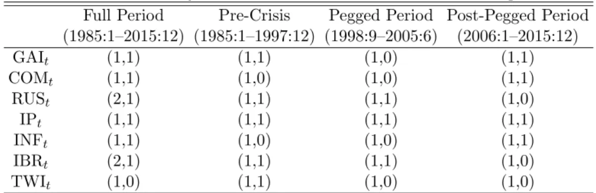
(m, j) = (1,1). From these, four are new components of order (1,1), as one is carried over from the SCM(1,0). There are seven SCMs of order (2,1) at position (m, j) = (2,1). Out of these two are new components of this order. Hence, the identified VARMA(2,1) consists of one SCM(1,0), four SCM(1,1) and two SCM(2,1).
A similar process is followed for each of the three sub-periods with all identified orders shown in Table (3). The overall orders for each of the three sub-periods are VARMA(1,1) while the orders of embedded SCMs differ across each of these. The pre-crisis period, consists of two SCM(1,0) and five SCM(1,1), the pegged exchange period consists of four SCM(1,0) and three SCM(1,1) and the post-pegged period consist of three SCM(1,0) and four SCM(1,1).
Table 3: A summary of the SCM orders identified for each sub-period. Full Period Pre-Crisis Pegged Period Post-Pegged Period (1985:1–2015:12) (1985:1–1997:12) (1998:9–2005:6) (2006:1–2015:12) GAIt (1,1) (1,1) (1,0) (1,1) COMt (1,1) (1,0) (1,0) (1,1) RUSt (2,1) (1,1) (1,1) (1,0) IPt (1,1) (1,1) (1,1) (1,1) INFt (1,1) (1,0) (1,0) (1,1) IBRt (2,1) (1,1) (1,1) (1,0) TWIt (1,0) (1,1) (1,0) (1,0)
Each variable forms an SCM within the identified VARMA structure. For example for the pre-crisis period IBRt loads as an SCM(1,1) while in the post-pegged period it loads as an SCM(1,0).
Implementing Stage II of the Athanasopoulos and Vahid (2008a) identification process described in Appendix A leads to additional zero restrictions on the matrix containing the contemporaneous relationships between the variables and the canonical SCM representa-tion of the identified VARMA models. We also ensure that the individual tests described in Appendix A do not contradict the normalization of the diagonal parameters of the
con-temporaneous matrix to one. The foreign block exogeneity restrictions are also imposed by excluding all domestic variables from entering the foreign block of equations. The SVARMA model specified for the full period is given by13
1 0 0 0 0 0 0 0 1 0 0 0 0 0 0 0 1 0 0 0 0 0 0 0 1 0 0 0 0 0 0 0 1 0 0 0 0 0 0 0 1 0 0 0 0 0 0 0 1 Xt=c+ α11(1) α(1)12 α(1)13 0 0 0 0 α21(1) α(1)22 α(1)23 0 0 0 0 α31(1) α(1)32 α(1)33 0 0 0 0 α41(1) α(1)42 α(1)43 α(1)44 α(1)45 α(1)46 α(1)47 α51(1) α(1)52 α(1)53 α(1)54 α(1)55 α(1)56 α(1)57 α61(1) α(1)62 α(1)63 α(1)64 α(1)65 α(1)66 α(1)67 α71(1) α(1)72 α(1)73 α(1)74 α(1)75 α(1)76 α(1)77 Xt−1 0 0 0 0 0 0 0 0 0 0 0 0 0 0 α31(2) α(2)32 α(2)33 0 0 0 0 0 0 0 0 0 0 0 0 0 0 0 0 0 0 α61(2) α(2)62 α(2)63 α(2)64 α(2)65 α(2)66 α(2)67 0 0 0 0 0 0 0 Xt−2 +υt− µ(1)11 µ(1)12 µ(1)13 0 0 0 0 µ(1)21 µ(1)22 µ(1)23 0 0 0 0 µ(1)31 µ(1)32 µ(1)33 0 0 0 0 µ(1)41 µ(1)42 µ(1)43 µ(1)44 µ(1)45 µ(1)46 µ(1)47 µ(1)51 µ(1)52 µ(1)53 µ(1)54 µ(1)55 µ(1)56 µ(1)57 µ(1)61 µ(1)62 µ(1)63 µ(1)64 µ(1)65 µ(1)66 µ(1)67 0 0 0 0 0 0 0 υt−1.
For the specification of the SVAR models, the standard information criteria AIC and HQ (Hannan-Quinn) select an optimal lag length of two, while the BIC selects a lag length of one for the whole period and all sub-periods. However the LM tests for serial autocorrelation in the residuals show that at least a lag length of six is required to capture all the dynamics in the data. Hence a VAR(6) is estimated for each of the sub-periods.
5
Empirical results
In this section, we present, compare and analyse key impulse response functions of do-mestic variables to independent shocks, derived from SVARMA and SVAR specifications. We also present and discuss historical and variance decompositions derived from SVARMA models for each of the sub-periods.
13
The representation for the sub-periods can be set-up by referring to the summary of the SCM orders provided in Table 3.
5.1 Impulse responses of domestic variables to foreign and domestic shocks
The sizes of the shocks are measured by one-standard deviation of the orthogonal errors of the respective models and are presented in Table 4. The sizes of the orthogonal shocks in the SVARMA and SVAR models appear to be similar. The impulse responses are normalized by dividing them with the standard deviation of the respective shocks and are shown in Figures 1 to 4. We observe the behavior of these responses over a period of 48 months. 68% confidence bands are computed via bootstrapping 10000 samples, using the bootstrap-after-bootstrap method of Kilian (1998).14.
Table 4: Magnitude of one standard deviation shocks from the SVARMA and SVAR models
Model GAI COM RUS IP INF IBR TWI
SVARMA 0.27 0.14 0.23 0.14 0.31 0.02 0.17 SVAR 0.26 0.15 0.22 0.13 0.29 0.02 0.17
Broadly speaking, a comparison of the results of the two alternative models indicates the benefits from using the SVARMA model over its SVAR counterpart. In many cases the SVARMA model appears to be performing better, particularly the responses of domestic variables to monetary shocks. We highlight these in the discussion that follows. Further-more, the confidence bands around the SVARMA responses appear to be narrower than those around the SVAR responses. In many other cases both SVARMA and SVAR models generate qualitatively similar impulse-response functions. These provide good ground for a robustness check of the empirical results from the two models.
5.1.1 Responses of domestic variables to a foreign and domestic monetary policy shocks
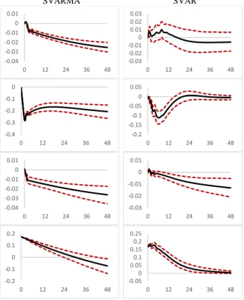
The responses of domestic variables to RUS and IBR shocks are shown in Figure 1. A positive RUS shock, which is defined as an unanticipated monetary contraction, leads to a rise in the US interest rate, resulting in excess demand for US currency in the foreign exchange market. The US dollar is expected to appreciate, while the Ringgit is expected to depreciate. As revealed by the SVARMA model, both interest rate and exchange rate are sensitive to foreign monetary shocks. IBR increases around 0.25% . The TWI contin-ues to depreciate and persists at around 0.5% below trend. Though BNM attempted to
14
Notes: SVARMA and SVAR impulse responses are shown as unbroken black and blue lines respectively with confidence bands shown as dashed lines
lean against exchange rate depreciation, the interest rate differential between the US and Malaysia appears to be causing the Ringgit to have persistent negative responses. This out-come is in line with Banerjee et al. (2016), who show evidence that a contractionary foreign monetary policy leads to an exchange depreciation in emerging economies. The depreciat-ing Rdepreciat-inggit could also explain the immediate rise in INF and IP, though not significant, as the rising Malaysian interest rate eventually offset the positive responses.
Figure 1: Responses of domestic variables to foreign and domestic monetary shocks
Fed Fund Rate (RUS) Shock Domestic Interest Rate (IBR) Shock
SVARMA SVAR SVARMA SVAR
O ut put (I P ) In fla tio n (I N F ) In te re st R ate (I B R ) E xc ha nge R at e (T W I)
Notes: SVARMA and SVAR impulse responses are shown as solid lines with 68% confidence bands (dashed lines) obtained from 10000 bootstrap replications. -0.06 -0.04 -0.02 0 0.02 0.04 0 12 24 36 48 -0.06 -0.04 -0.02 0 0.02 0.04 0 12 24 36 48 -0.03 -0.02 -0.01 0 0.01 0 12 24 36 48 -0.02 0 0.02 0.04 0 12 24 36 48 -0.06 -0.04 -0.020 0.02 0.04 0.06 0 12 24 36 48 -0.1 -0.05 0 0.05 0 12 24 36 48 -0.025 -0.02 -0.015 -0.01 -0.005 0 0 12 24 36 48 -0.1 -0.05 0 0.05 0 12 24 36 48 0 0.01 0.02 0.03 0 12 24 36 48 -0.005 0 0.005 0.01 0.015 0 12 24 36 48 0 0.01 0.02 0.03 0 12 24 36 48 0 0.005 0.01 0.015 0.02 0 12 24 36 48 -0.1 -0.05 0 0.05 0 12 24 36 48 -0.1 -0.05 0 0.05 0 12 24 36 48 -0.015 -0.01 -0.005 0 0.005 0.01 0 12 24 36 48 -0.04 -0.02 0 0.02 0.04 0 12 24 36 48
Shocks to IBR are treated as unanticipated changes to Malaysian monetary policy. A short-run increase of 0.25% in IBR, itself has a persistent effect. As observed in the SVARMA model, immediately TWI appreciates, as influenced by market forces, and IP contracts. The SVAR signals the presence of an output puzzle and non-response exchange rate. A negative response of INF is observed in the both models, while the effect appears to be less intensive for the SVARMA model (around 0.1%). However it does seem to be more persistent compared to that obtained via the SVAR model. The negative persistent response of IP may be due to a rise in the real cost of borrowing, the appreciation of the Ringgit, and a degree of price rigidity in the economy. The TWI responses are in line with the Dornbusch (1976) overshooting hypothesis, where on impact it appreciates around 0.1%
above trend. As a small open economy with capital mobility, an unanticipated increase in domestic interest rates will attract investors to domestic assets, inducing net inflows on the capital account leading to an initial appreciation of domestic currency. Subsequent depreciation of the Ringgit is expected, in line with uncovered interest rate parity and purchasing power parity (see for example Dumrongrittikul and Anderson, 2016). Overall, the monetary responses highlight the adequacy of SVARMA over SVAR for identifying an appropriate monetary policy shock and producing impulse responses, which are consistent with macroeconomic theoretical model predictions.
5.1.2 Responses of domestic variables to a global activity and domestic output shocks
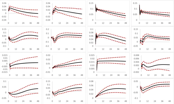
The responses of the domestic variables to GAI and IP shocks which are defined as foreign and domestic demand shocks respectively. These are shown in Figure 2. A positive GAI shock leads to rise in IP and fall in TWI while the effect on INF and IBR are largely muted. The IP rise to around 0.4% above trend after three months and then starts to decline and return to its normal path within twenty four months.
A positive 1.4% IP shock causes inflationary pressure in the economy, where INF in-creases by 0.6% on impact. IBR increases around 0.15%, consistent with the contractionary policy measure usually undertaken by central banks against expanding economies. The rise in interest rate, leads to a rise in TWI around 0.4% above trend and for both IBR and TWI, the effects are persistent. Due to the contractionary monetary policy and the appreciation of the exchange rate, inflation starts declining after twelve months. These results are clearly demonstrated via SVARMA while exchange rate puzzle exist following a contractionary monetary policy in the SVAR model.
Overall, as expected, IP is sensitive to both global and domestic demand shocks. Since the INF, IBR and TWI are significantly affected by domestic demand shock, the effects of global demand shocks are presumed to be felt indirectly via IP.
5.1.3 Responses of domestic variables to a commodity price and domestic inflation shocks
The responses of domestic variables to COM and INF shocks which are defined as foreign and domestic supply shocks respectively. These are shown in Figure 3. By examining the responses to these price shocks, we can reasonably ascertain whether the specifications of
Figure 2: Responses of domestic variables to global activity and domestic output shocks
Global Activity (GAI) Shock Domestic Output (IP) Shock
SVARMA SVAR SVARMA SVAR
O ut put (I P ) In fla tio n (I N F ) In te re st R ate (I B R ) E xc ha nge R at e (T W I)
Notes: SVARMA and SVAR impulse responses are shown as solid lines with 68% confidence bands (dashed lines) obtained from 10000 bootstrap replications. -0.04 -0.02 0 0.02 0.04 0.06 0 12 24 36 48 -0.04 -0.02 0 0.02 0.04 0.06 0 12 24 36 48 0 0.05 0.1 0.15 0 12 24 36 48 0 0.05 0.1 0.15 0 12 24 36 48 -0.1 -0.05 0 0.05 0.1 0.15 0 12 24 36 48 -0.2 -0.1 0 0.1 0.2 0 12 24 36 48 0 0.02 0.04 0.06 0.08 0.1 0 12 24 36 48 -0.05 0 0.05 0.1 0.15 0 12 24 36 48 -0.015-0.01 -0.0050 0.0050.01 0.015 0 12 24 36 48 -0.01 0 0.01 0.02 0.03 0 12 24 36 48 0 0.005 0.01 0.015 0.02 0.025 0 12 24 36 48 -0.002 0 0.002 0.004 0.006 0.008 0 12 24 36 48 -0.05 0 0.05 0.1 0 12 24 36 48 -0.1 -0.05 0 0.05 0.1 0.15 0 12 24 36 48 0 0.02 0.04 0.06 0.08 0 12 24 36 48 -0.1 -0.05 0 0.05 0 12 24 36 48
monetary policy equation in our SVARMA and SVAR models provide accurate representa-tion of how BNM determines its monetary policy in containing inflarepresenta-tionary pressure.
Since the world commodity price is based on the world market price, a positive COM shock leads to an inflationary pressure in the Malaysian economy. As expected, to combat the rise in inflation, BNM responded by increasing the policy rate around 0.3% on impact. Considering that Malaysia is a net commodity importer, a positive COM shock leads to a negative movement in output, where within three months, IP falls below trend by 0.5%. As observed in Figure 3, rise in interest rate and inflation rate, lead to an immediate rise of the real exchange rate. This leads to a fall in consumption, investment and exports, causing a persistent negative effects on output. Unlike the global demand shock, domestic variables are more sensitive to global supply shock.
A positive shock to INF can be regarded as unanticipated inflationary pressure on the economy and as a consequence, IBR is expected to rise. The unanticipated rise in inflation results in an approximate 0.25% appreciation of the real exchange rate, partly due to the rise in interest rate. This is followed by a decline in output, where it falls around 0.3% below trend. As the interest rate starts declining, the exchange rate also
Figure 3: Responses of domestic variables to world commodity and domestic inflation shocks
World Commodity Price (COM) Shock Domestic Inflation (INF) Shock
SVARMA SVAR SVARMA SVAR
O ut put (I P ) In fla tio n (I N F ) In te re st R ate (I B R ) E xc ha nge R at e (T W I)
Notes: SVARMA and SVAR impulse responses are shown as solid lines with 68% confidence bands (dashed lines) obtained from 10000 bootstrap replications. -0.1 -0.05 0 0.05 0 12 24 36 48 -0.06 -0.02 0.02 0.06 0 12 24 36 48 -0.15 -0.1 -0.05 0 0 12 24 36 48 -0.03 -0.02 -0.01 0 0.01 0.02 0 12 24 36 48 -0.1 -0.05 0 0.05 0.1 0 12 24 36 48 -0.05 0 0.05 0.1 0.15 0.2 0 12 24 36 48 -0.2 0 0.2 0.4 0.6 0 12 24 36 48 -0.1 0 0.1 0.2 0.3 0.4 0 12 24 36 48 0 0.01 0.02 0.03 0.04 0 12 24 36 48 -0.005 0 0.005 0.01 0.015 0.02 0 12 24 36 48 0 0.02 0.04 0.06 0 12 24 36 48 -0.005 0 0.005 0.01 0 12 24 36 48 -0.1 -0.05 0 0.05 0.1 0 12 24 36 48 -0.05 0 0.05 0.1 0.15 0 12 24 36 48 -0.08 -0.06 -0.04 -0.020 0.02 0.04 0 12 24 36 48 -0.04 -0.02 0 0.02 0.04 0.06 0 12 24 36 48
declines. The ‘hump-shaped’ responses of interest rate, generated via SVARMA, peaked around three months after which it slowly declines. These outcomes are in line with those found for export oriented economies (see for example Chevaptrukul et al., 2009; William and Schereyer, 2012). A higher interest rate, leads to domestic currency appreciation and in the effort to limit the exchange rate, the central bankers in export oriented economies like Malaysia would eventually slowly loosen their monetary policy. A comparison of both models’ responses shows only via the SVARMA model, a significant dynamic response of monetary policy is observed.
Overall, the Malaysian economy is vulnerable to both foreign and domestic inflationary pressure. It is evident that these expected movements of domestic variables to both infla-tionary shocks are well captured by impulse responses generated by the SVARMA model.
5.1.4 Responses of domestic variables to a foreign exchange shock
A currency appreciation is expected to have two opposing effects on output. On the one hand, it is expected to decrease exports, as these become relatively more expensive than imports. On the other hand, it also expected to help reduce the cost of production through
lower prices of imported intermediate goods. These combined effects transmitted via the demand and supply channels would determine the net influence of an exchange rate shock on output. As shown in Figure 4, the decline in Malaysian output, generated via SVARMA model, implies the negative effects coming through the demand channel offset the positive effects coming through the supply channel.
Figure 4: Responses of domestic variables to an exchange rate shock
Exchange Rate (TWI) Shock
SVARMA SVAR O ut put (I P ) In fla tio n (I N F ) In te re st R ate (I B R ) E xc ha nge R at e (T W I)
Notes: Refer to the notes in the previous Figures. -0.04 -0.03 -0.02 -0.01 0 0.01 0 12 24 36 48 -0.03 -0.02 -0.010 0.01 0.02 0.03 0 12 24 36 48 -0.4 -0.3 -0.2 -0.1 0 0 12 24 36 48 -0.2 -0.15 -0.1 -0.05 0 0.05 0 12 24 36 48 -0.04 -0.03 -0.02 -0.01 0 0.01 0 12 24 36 48 -0.03 -0.02 -0.01 0 0.01 0 12 24 36 48 -0.2 -0.1 0 0.1 0.2 0 12 24 36 48 -0.05 0 0.050.1 0.150.2 0.25 0 12 24 36 48
As expected, inflation responds negatively to an exchange rate shock due to lower import prices and production costs. IBR is expected to decline in response to a positive TWI shock where on one hand, an unanticipated appreciation of currency should prompt policy makers to lean against currency appreciation while the other is to stimulate the sluggish output and inflation.
Based on the results obtained via the SVARMA model, we can broadly conclude that domestic variables are responsive to both domestic and foreign shocks. Further, both do-mestic output and price levels are two important indicators for monetary policy operations in Malaysia.
5.2 Historical decomposition of domestic variables
In this section we undertake a historical decomposition analysis of the relative contributions of the foreign and domestic shocks to domestic variables. As discussed in Section 2, Malaysia adopted economic and financial reforms following the Asian financial crisis of the late 1990s. Thus, it is important to see whether the economy has become more or less vulnerable to foreign shocks over time under the different exchange rate regimes. It is expected that an increasing economic openness, along with a relatively greater integration with the global economy, would increase the contributions of foreign shocks on the domestic economy.
Figure 5 shows the respective historical decomposition of output and inflation to foreign and domestic shocks. The SVARMA model is used to decompose these two variables into their component shocks. Notable differences are observed in the way foreign and domestic shocks impact the Malaysia economy over time. Following the unpegging of the Ringgit in 2005, foreign shocks appear to cause sharply defined upward movements to both output and inflation. Decomposing the shocks further, highlights that output and inflation were largely exposed to global activity and world commodity price shocks respectively. In the lead-up to the 1998 crisis, world commodity price caused a downward movement in output. A similar pattern is also observed for inflation.
Prior to 1998, domestic factors contributed positively to output. During the Asian crisis period, there is a sharp decline in output, mainly contributed by domestic factors. This may reflect rapid shifts in the market’s assessment of the uncertainty about business cycle movements during the crisis period. Inflation also rose due to economic uncertainty caused by the crisis. The exchange rate appears to have negative effects on output, prior to the scrapping of the Ringgit’s peg to the US dollar. Following the GFC, the exchange rate was again contributing negatively to output while inflation contributed positively to output. As for inflation, the output shock plays an important role and in recent times led to a downward movements in inflation.
Figure 6 shows the relative contributions of foreign and domestic shocks to interest rate and exchange rate. For both variables, foreign shocks historically made comparatively bigger contributions while the domestic shocks made relatively smaller contributions. Dur-ing the pegged-exchange rate period (1998:9–2005:6), the contribution of foreign shocks to these two variables is negative while in the post-pegged period it is positive. Prior to 2005,
Figure 5: Historical decomposition of output and inflation to foreign and domestic shocks Contribution to Output (IP) Contribution to Inflation (INF)
-1.5 -1 -0.5 0 0.5 1 1.5 85 90 95 00 05 10 15
Own Foreign Domestic
-6 -4 -2 0 2 4 6 85 90 95 00 05 10 15
Own Foreign Domestic
-0.8 -0.6 -0.4 -0.20 0.2 0.4 0.6 0.81 1.2 85 90 95 00 05 10 15
GAI COM RUS
-1.5 -1 -0.5 0 0.5 1 1.5 2 2.5 85 90 95 00 05 10 15
GAI COM RUS
-0.3 -0.2 -0.1 0 0.1 0.2 85 90 95 00 05 10 15
INF IBR TWI
-0.6 -0.4 -0.2 0 0.2 0.4 0.6 0.8 85 90 95 00 05 10 15 IP IBR TWI
the main foreign drivers for the interest rate are US monetary policy surprises and global activity shock while for the exchange rate is the world commodity prices. In the post-pegged period (2006:1–2015:12) however, exchange rate is largely driven by global activity and in the post 2008 GFC period, foreign monetary shock and commodity price shocks play important roles. This outcome is not surprising as during the post-GFC period, ad-vanced economies embarked on quantitative easing. This resulted in large capital inflows to emerging economies, seeking for better returns. About the same time, the global economy was also witnessing the fall in commodity prices. Consequently these two factors cause the Malaysian exchange rate to appreciate.
Between domestic output and inflation, output tends to have bigger influence on interest rate and exchange rate. In the pre-crisis period (1985:1–2015:12) and in the post-pegged period (2006:1–2015:12), that is during the managed float exchange rate regime, output contributed negatively to interest rate and exchange rate while during the pegged period, it contributed positively to these two variables. Interest rate also plays an important role for exchange rate where during the 1998 Asian crisis and 2008 Global crisis it contributed negatively to exchange rate and since 2010 it has been contributing positively to exchange rate movements.
Overall, the contribution of foreign shocks appear to be larger than domestic shocks. Among the domestic shocks, the main driver of the economy is domestic output followed by the exchange rate. The way the various shocks contribute to the economy, clearly demonstrates the three sub-period specified in Section 4.
5.3 Forecast Error Variance Decomposition
In Table 5, the forecast error variance decomposition of the four domestic variables, for the pre-crisis, pegged and post-pegged periods are presented. Results are reported for forecast horizons 6, 12 and 48 months ahead. The results appear to have a varied path between the three sub-periods.
Focussing first on the pre-crisis period, the decompositions of the domestic variables show that over a six months horizon, between 75.534% to 90.12% of the variances are attributable to their own shocks. There is evidence that in the longer horizon of four years, COM is an important source of domestic fluctuations (i.e. its contribution varies between 23.56% to 29.84%). INF and the TWI seem to be the two variables mostly affected
Figure 6: Historical decomposition of interest and exchange rate to foreign and domestic shocks
Contribution to Interest Rate (IBR) Contribution to Exchange Rate (TWI)
-0.5 -0.4 -0.3 -0.2 -0.10 0.1 0.2 0.3 0.4 0.5 85 90 95 00 05 10 15
Own Foreign Domestic
-2 -1.5-1 -0.50 0.51 1.52 2.53 85 90 95 00 05 10 15
Own Foreign Domestic
-0.5 -0.4 -0.3 -0.2 -0.10 0.1 0.2 0.3 0.4 0.5 85 90 95 00 05 10 15
GAI COM RUS
-2 -1.5-1 -0.50 0.51 1.52 2.53 85 90 95 00 05 10 15
GAI COM RUS
-0.06 -0.04 -0.02 0 0.02 0.04 0.06 85 90 95 00 05 10 15 IP INF TWI -0.8 -0.6 -0.4 -0.2 0 0.2 0.4 0.6 0.8 85 90 95 00 05 10 15 IP INF IBR
Table 5: Variance decomposition of the domestic variables during the pre- pegged and post-pegged periods
Period Pre-Crisis Pegged Post-Pegged
(1985:1–1997:12) (1998:9–2005:6) (2006:1–2015:12) Horizon 6 12 48 6 12 48 6 12 48 Shocks IP GAI 1.92 1.45 0.99 5.02 6.45 4.06 21.25 20.87 21.19 COM 15.05 35.36 25.64 2.35 2.04 3.81 16.09 13.34 52.60 RUS 1.52 3.51 10.27 32.42 30.08 43.38 9.91 30.75 18.12 IP 75.53 46.04 10.78 41.31 27.06 12.56 44.30 26.65 5.08 INF 0.32 0.95 9.69 17.87 32.99 34.42 2.26 2.33 0.48 IBR 0.59 3.11 7.80 0.31 0.81 0.73 6.04 5.91 2.02 TWI 5.05 9.59 34.82 0.71 0.55 1.03 0.15 0.10 0.48 INF GAI 1.10 2.68 2.89 0.01 0.41 5.32 8.73 25.19 27.07 COM 0.16 1.98 23.56 10.89 16.51 16.08 13.06 26.19 27.93 RUS 8.12 17.48 23.15 1.07 2.57 29.47 5.44 5.96 16.89 IP 7.45 8.05 4.25 0.85 0.50 2.33 3.57 3.84 2.52 INF 82.29 68.13 35.98 86.65 78.41 37.31 63.68 32.66 15.56 IBR 0.74 0.85 1.28 0.06 0.45 8.54 0.76 2.63 5.82 TWI 0.12 0.81 8.86 0.44 1.12 0.92 4.77 3.54 4.20 IBR GAI 1.45 0.84 1.58 8.37 16.24 29.13 0.08 1.76 9.03 COM 1.76 1.11 29.84 1.73 8.00 5.14 0.21 0.11 31.13 RUS 1.60 2.04 2.72 6.21 9.07 7.89 0.05 0.69 18.21 IP 1.36 1.48 0.63 0.77 3.16 9.17 7.61 6.66 1.96 INF 2.12 3.61 9.89 21.36 19.96 12.05 0.57 0.69 0.75 IBR 90.12 89.83 35.04 57.28 41.06 35.71 86.48 76.04 25.51 TWI 1.58 1.08 20.28 4.26 2.49 0.93 4.98 14.04 13.38 TWI GAI 1.88 2.66 3.11 21.13 30.58 21.44 0.70 1.16 18.03 COM 0.81 3.55 28.13 0.09 0.06 12.94 14.28 34.64 66.49 RUS 7.17 17.51 43.98 0.54 0.54 27.42 2.42 5.76 3.42 IP 0.03 0.01 0.00 0.41 0.41 3.48 2.85 1.77 0.38 INF 9.90 10.55 3.98 11.74 11.74 12.17 1.43 1.23 0.28 IBR 0.18 0.09 0.02 4.84 4.84 13.77 0.61 0.41 0.49 TWI 80.00 65.61 20.77 61.23 61.23 8.78 77.69 55.02 10.90
by foreign monetary shocks, with RUS contributing 23.15% and 43.98% of the variation respectively at a four year horizon. On the other hand, for IP and IBR, the exchange rate seems to have a greater role. This implies that the foreign monetary shocks are channeled via the exchange rate to the domestic economy. The global activity index has relatively a minimal effect on all domestic variables, consistent with the results obtained via historical decomposition shown in Figures 5 and 6.
Different results are projected during the pegged exchange rate period. Over a four year horizon, the foreign monetary shocks contributed 43.38%, 29.47% and 27.42% to IP, INF and TWI respectively. The global activity shock is an important source of fluctuation for IBR (29.13%) and TWI (21.44%). While the effects of the world commodity prices declined, the domestic inflation shock appear to be an important source of fluctuations
particularly on IP (34.42%) over the four year horizon. As expected, the exchange rate played minimal role on other domestic variables where its contribution only varies between 0.92% and 1.03%. For IBR, at 48 months, 21.22% of the fluctuations is due to a combined effects from domestic output and inflation, implying that BNM had some breathing space to focus on domestic variables, compared to the pre-crisis (3.98%) and the post-pegged (0.66%) periods.
In the post-pegged period, the main drivers of domestic fluctuation are foreign shocks where over the four year period, their combined effects contributed around 91.91%, 71.89%, 58.37% and 85.94% variations on IP, INF, IBR and TWI respectively. During this period, the world commodity price was the most influential foreign variable. This outcome is in line with the rise in the global energy price during 2006-2008 period (Kilian and Murphy, 2014) and consistent with that reported in Raghavan and Dungey (2015). The global activity shocks largely affected IP, INF and TWI, with comparatively minimal effects on IBR while the foreign monetary shock causes less fluctuations on TWI compared to other domestic variables.
6
Conclusion
The use of SVARs to model emerging or transitional small open economies can be challeng-ing as these economies are usually plagued by frequent policy changes, structural breaks or the general lack of data availability. In this regard, the use of a more parsimonious SVARMA model is deemed suitable. We use a SVARMA model to examine the trans-mission of foreign and domestic shocks to Malaysia, a small open emerging economy. To demonstrate the benefits of using a SVARMA model we compare the impulse responses gen-erated by a SVARMA model with those gengen-erated by a SVAR. We find that the SVARMA model produces impulse responses that are consistent with prior theoretical expectations and stylized facts. The empirical results based on the SVARMA methodology show notable differences in the foreign and domestic shock transmission under the different exchange rate regimes experienced by Malaysia.
The changes in the Malaysian economic structure, financial system and exchange rate regime seem to have an important influence in shaping the relationship between the foreign variables and the domestic economic and financial variables. For example, BNM appears to
have less power to influence inflation and the exchange rate under a managed exchange rate regime with high capital mobility. While, during the pegged exchange rate period, BNM experienced some breathing space to focus on maintaining price and output stability. Based on the responses obtained from the SVARMA model, it is apparent that in the post-pegged period, the Malaysian economy is highly affected by external shocks, highlighting Malaysia’s increasing exposure to external demand and policy changes. This implies that, similar levels of monetary policy changes will have differing effects on the economy, depending on the type of policy regimes.
The successful construction and implementation of the SVARMA model for Malaysian business cycle analysis, along with its promising impulse responses indicates the suitability of this framework for other similar open emerging economies and transitional economies, especially for those economies that are not currently investigated due to limited data avail-ability. Considering the differences in the effects of foreign and domestic shocks under the different policy regimes, it is essential for policymakers to understand how the eco-nomic transformation, openness of the economy and the growing integration with external economies affects the nature of the shock transmission mechanism. It would therefore be beneficial to study these features of emerging economies, coupled with appropriate mod-elling techniques to uncover key issues that have implications for the conduct of economic policy.
References
ADB (Ed.) (2017). Asian Economic Integration Report: The Era of Financial
Inter-connectedness - How can Asia Strengthen Financial Resilience? Asian Development
Bank.
Athanasopoulos, G. and F. Vahid (2008a). A complete VARMA modelling methodology based on scalar components. Journal of Time Series Analysis 29, 533–554.
Athanasopoulos, G. and F. Vahid (2008b). VARMA versus VAR for macroeconomic forecasting. Journal of Business and Economic Statistics 26, 237–252.
Athukorala, P. C. (2001). Crisis and recovery in Malaysia: The role of capital controls. Cheltenham, UK: Edward Elgar.
Azali, M. (2003). Transmission Mechanism in a Developing economy : Does Money or
Credit Matter? Second Ed, UPM, Press.
Banerjee, R., M. Devereux, and G. Lombardo (2016). Self-oriented monetary policy, global financial market and excess volatility of international capital flows. Journal of
International Money and Finance 68, 275–297.
Bernanke, B. S. and I. Mihov (1998). Measuring monetary policy. The Quarterly Journal
of Economics 113 (3), 869–902.
Cheong, L. M. (2004). Globalisation and the operation of monetary policy in Malaysia.
Bank of International Settlements, BIS Papers Series 23, 209–215.
Chevaptrukul, T., T. Kim, and P. Mizen (2009). The Taylor principle and monetary policy approaching a zero bound on nominal rates: quantile regression results for the United States and Japan. Journal of Money, Credit and Banking 41, 1705–1723. Cooley, T. and M. Dwyer (1998). Business cycle analysis without much theory. A look
at structural VARs. Journal of Econometrics 83, 57–88.
Cushman, D. O. and T. A. Zha (1997). Identifying monetary policy in a small open economy under flexible exchange rates. Journal of Monetary Economics 39(3), 433– 448.
Dekle, R. and M. Pradhan (1997). Financial liberalization and money demand in ASEAN countries: Implications for monetary policy. IMF Working Paper WP/97/36. Domac, I. (1999). The distributional consequences of monetary policy: Evidence from
Malaysia. The World Bank Policy Research Working Papers 2170.
Dornbusch, R. (1976). Expectations and exchange rate dynamics. Journal of Political
Economy 84(6), 1161–1176.
Downes, P. (2007, May). ASEAN fiscal and monetary policy responses to rising oil prices.
REPSF Report Project No. 06/004.
Dufour, J. M. and D. Pelletier (2002). Linear methods for estimating varma models with a macroeconomic application. Joint Statistical Meetings - Busniess amd Economic Statistics Section, 2659–2664.
Dufour, J.-M. and D. Pelletier (2011). Practical methods for modelling weak VARMA processes: Identification, estimation and specification with a macroeconomic applica-tion. Discussion Paper, Department of Economics, McGill University , CIREQ and CIRANO.
Dumrongrittikul, T. and H. M. Anderson (2016). How do shocks to domestic factors affect real exchange rates of Asian developing countries? Journal of Development
Economies 119.
Dungey, M. and A. Pagan (2009). Extending a SVAR model of the Australian economy.
The Economic Record 85 (268), 1–20.
Fern´andez-Villaverde, J., J. F. Rubio-Ram´ırez, and T. J. Sargent (2007). A,B,C’s (and D)’s for understanding VARs. The American Economic Review 308.
Fry, R. and A. Pagan (2005). Some issues in using VARs for macroeconometric reseach.
Australian National University, CAMA Working Paper Series 19/2005.
Granger, C. W. J. and M. J. Morris (1976). Time series modeling interpretation. Journal of the Royal Statistical Society 139(2), 246–257.
Hannan, E. J. and M. Deistler (1988). The statistical theory of linear systems. New York: John Wiley & Sons.
Ibrahim, M. (2005). Sectoral effects on monetary policy: Evidence from Malaysia. Asian
Economic Journal 19(1), 83–102.
Kapetanios, G., A. Pagan, and A. Scott (2007). Making a match: Combining theory and evidence in policy-oriented macroeconomic modeling. Journal of Econometrics 136, 565–594.
Kilian, L. (1998). Small-sample confidence intervals for impulse response functions.
Re-view of Economics and Statistics 80, 218–230.
Kilian, L. (2009). Not all oil price shocks are alike: disentangling demand and supply shocks in the crude oil market. American Economic Review 99(33), 1053–1069. Kilian, L. and D. Murphy (2014). The role of inventories and speculative trading in the
Kim, S. and N. Roubini (2000). Exchange rate anomalies in the industrial countries: A solution with a structural VAR approach. Journal of Monetary Economics 45(3), 561–586.
Krippner, L. (2013). Measuring the stance of monetary policy in zero lower bound environments. Economics Letters 118(1), 135–138.
L¨utkepohl, H. (2005). The New Introduction to Multiple Time Series Analysis. Berlin: Springer-Verlag.
Maravall, A. (1993). Stochastic linear trends: Models and estimators. Journal of Econo-metrics 56, 5–37.
McCauley, R. N. (2006). Understanding monetary policy in Malaysia and Thailand: Objectives, instruments and independence. Bank of Internatonal Settlements, BIS
Papers Series 31, 172–198.
Mehrotra, A. and J. Sanchez-Fung (2011). Assessing McCallum and Taylor rules in a cross-section of emerging market economies. Journal of International Financial
Markets, Institutions and Money 21, 207–228.
Ooi, S. (2008). The monetary transmission mechanism in Malaysia: Current develop-ments and issues. BIS Papers, Bank of International Settlement 35, 345–361.
Raghavan, M., G. Athanasopoulos, and P. Silvapulle (2016). Canadian monetary policy analysis using a structural VARMA model. Canadian Journal of Economics 49(1), 347–373.
Raghavan, M. and M. Dungey (2015). Should ASEAN-5 monetary policymakers act pre-emptively against stock market bubbles? Applied Economics 47 (11), 1086 – 1105.
Raghavan, M., P. Silvapulle, and G. Athanasopoulos (2012). Structural var models for malaysian monetary policy analysis during the pre- and post-1997 asian crisis periods.
Applied Economics 44(29), 3841–3856.
Reinsel, G. C. (1997). Elements of Multivariate Time Series (2nd ed.). New York: Springer-Verlag.