Data in a Joint Detection Estimation Framework
L. Chaari1, F. Forbes1, T. Vincent1, and P. Ciuciu21 Mistis team, Inria Grenoble and LJK, France 2 CEA/DSV/I2BM/Neurospin, LNAO, Gif-Sur-Yvette, France
Abstract. Identifying brain hemodynamics in event-related functional MRI (fMRI) data is a crucial issue to disentangle the vascular response from the neuronal activity in the BOLD signal. This question is usu-ally addressed by estimating the so-called Hemodynamic Response Func-tion (HRF). Voxelwise or region-/parcelwise inference schemes have been proposed to achieve this goal but so far all known contributions com-mit to pre-specified spatial supports for the hemodynamic territories by defining these supports either as individual voxels or a priori fixed brain parcels. In this paper, we introduce a Joint Parcellation-Detection-Estimation (JPDE) procedure that incorporates an adaptive parcel iden-tification step based upon local hemodynamic properties. Efficient infer-ence of both evoked activity, HRF shapes andsupports is then achieved using variational approximations. Validation on synthetic and real fMRI data demonstrate the JPDE performance over standard detection esti-mation schemes and suggest it as a new brain exploration tool.
1
Introduction
Within-subject analysis in event-related BOLD fMRI mainly relies on (i) detec-tion of evoked activity to localize which parts of the brain are activated by a given stimulus type, and on (ii)estimationof the dynamics of the brain response also known as the Hemodynamic Response Function (HRF). Most approaches to detect neural activity rely on a singlea priori HRF model for the whole brain although there has been evidence that this response can vary between cortical re-gions and across subjects [8] and that an accurate HRF model may significantly improve detection performance. To capture this variability, robust HRF estima-tion is necessary which can be achieved only in voxels or regions that elicit an evoked response to a given stimulus [9]. So far, many works have addressed this issue either by considering linear or nonlinear HRF models [1, 4, 14], parametric, semi-parametric or non-parametric (i.e. FIR models) descriptions [6, 16, 7], and by performing univariate (voxelwise) [4, 16], multivariate (regionwise) [10, 13] or even multiscale, i.e. spatially adaptive inference [15]. However, to the best of our knowledge, all these existing works assume the spatial support of the HRFs, either defined at the voxel or region-level, to be pre-specified. The proposed methodology takes place in the Joint Detection-Estimation (JDE) framework in-troduced in [10] and extended in [13,3] to account for spatial correlation between
N. Ayache et al. (Eds.): MICCAI 2012, Part III, LNCS 7512, pp. 180–188, 2012.
voxels. Standard JDE-based inference requires a pre-specified decomposition of the brain into functionally homogeneous parcels (groups of connected voxels) but with no guarantee of their optimality. These parcels should be small enough to guarantee the invariance of the HRF within each parcel but large enough to contain reliable information for its inference [12]. Here, we introduce the concept ofhemodynamic territory as a set of parcels which share a common HRF pattern. To determine such sets, we incorporate an additional layer in the JDE hierar-chy, namely an adaptive parcel identification step based upon local hemody-namic properties. In this novel Joint Parcellation-Detection-Estimation (JPDE) model (Section 2), for all the parcels of a given territory, HRFs are voxelwise but defined as local stochastic perturbations of the same HRF pattern. Then, hemodynamics estimation reduces to the identification of a limited number (say
K) of such HRF patterns and parcel identification reformulates as a cluster-ing problem where each voxel is assigned an HRF group among K. The HRF group assignment variables are governed by a hidden Markov Model to enforce spatial correlation,i.e. favor group assignments to vary smoothly. Finally, the overall scheme iteratively identifies hemodynamic territories as pairs of one HRF pattern and a set of parcels assigned to the corresponding HRF group.
The proposed approach thus makes the JDE framework fully adaptive and more flexible. It is based on a variational Expectation Maximization (EM) algo-rithm (Section 3) to derive estimates of the HRF patterns, the response ampli-tude, the corresponding labels (activating/non-activating voxels) and the HRF group labels. Results on artificial and real fMRI data demonstrate that the JPDE approach outperforms the standard JDE (see Section 4).
2
A Joint Parcellation-Detection-Estimation model
2.1 Observed and Missing Variables
We extend the parcel-based JDE model of [10, 13] to a whole-brain one, with a set of voxels denoted byP, and recast it in a missing data framework. At voxel
j, the fMRI time seriesyj is measured at times{tn, n= 1:N}, wheretn=nTR,
N being the number of scans and TR the time of repetition. The number of different stimulus types or experimental conditions isM. At each voxelj, we assume a voxel dependent HRFhj ∈RD+1 withH={hj, j∈P}the set of all HRFs. Eachhj is associated with a HRF group amongK. These groups or HRF classes are specified by a set of hidden labelsZ={zj, j∈P}wherezj ∈ {1 :K} andzj =kmeans that voxel j belongs to the k-th group. An estimation of Z corresponds then to a partition of the brain into K hemodynamic territories whose connected components define a parcellation. The link to the observed BOLD data is specified via the following forward model:
∀j∈P, yj= M m=1 am jXmhj+Pj+εj, (1)
where the binary matrix Xm = {xnm−dΔt, n = 1 : N, d = 0 : D} is of size
m-th experimental condition, Δt < T R being the sampling period of the un-known HRFs. The scalar am
j ’s are weights that model the transition between stimulations and the neuro-vascular response. They are generally referred to as Neural Response Levels (NRL). We denote by A ={am, m= 1 :M} with am=am
j , j∈P
the response amplitudes,amj being the amplitude at voxelj for conditionm. Similarly to the HRF’s, each NRL is assumed to be in one ofI groups specified by activation class assignment variablesQ={qm, m= 1 :M} whereqm =qm
j , j∈P
and qm
j represents the activation class at voxel j for conditionm. The number of classes considered here isI= 2 for activated (i= 2) and non-activated (i= 1) voxels. Finally, the rest of the signal is made of vector Pj, which corresponds to low frequency drifts withP aN×Omatrix,j∈RO a vector to be estimated andL={j, j∈P}. Regarding the observation noise, the εj’s are assumed to be independent with εj ∼ N(0,Γ−j1). The set of all unknown precision matrices is denoted byΓ ={Γj, j∈P}.
2.2 Hierarchical Model of the Complete Data Distribution
With standard additional assumptions [10, 13, 3], the joint model distribution writesp(Y,A,H,Q,Z) =p(Y |A,H)p(A|Q)p(Q)p(H|Z)p(Z).
Likelihood. Assuming spatial independence of the noise, the likelihood reads p(Y |A,H;L,Γ) ∝ j∈PNyj; M m=1a m j Xmhj +Pj,Γ−1j . Various possibilities for theΓj’s include standard white and autoregressive noise models [10]. Neuronal Response Levels. The NRLs are assumed to be statisti-cally independent across conditions: p(A;θa) = Mm=1p(am;θm) where
θa ={θm, m= 1 :M} and θm gathers the parameters for the m-th condition. A mixture model is then adopted by using the allocation variables qjm to segregate non-activated voxels (qjm = 1) from activated ones (qmj = 2). For the m-th condition, and conditionally to the assignment variables qm, the NRLs are assumed to be independent: p(am|qm;θm) = j∈Pp(amj |qmj ;θm) withp(am
j |qmj =i;θm)∼ N(μmi, vmi) andθm ={μmi, vmi, i= 1,2}. We also denote μ={μmi, m= 1 :M, i= 1,2} and v = {vmi, m= 1 :M, i= 1,2}. For non-activating voxels (i= 1) we set for all m, μm1= 0. The other parameters
are unknown and have to be estimated.
Activation Classes. We assume prior independence between the M experimental conditions regarding the activation class assignments:
p(Q) =Mm=1p(qm;β
m).Also, the densityp(qm;βm)∝exp
βmU(qm)
defines a spatial Markov prior, namely an Ising model with interaction parameter βm and energy functionU(qm) =
j∼jδ(qmj , qjm) where∀(a, b)∈R2, δ(a, b) = 1 if a = b and 0 otherwise. The notation j ∼ j means that the summation is over all neighboring voxels (in a 6-connexity 3D neighborhood). The unknown parameters are denoted byβ={βm, m= 1 :M}.
HRF Groups. In order to promote parcellation connexity, we also introduce here a spatial Markov prior, namely a K-class Potts model with interac-tion parameter βz: p(Z;βz) ∝ expβzU(Z), where the global energy reads
U(Z) = j∼jδ(zj, zj), i.e. neighboring voxels tend to belong to the same HRF group.
HRF Patterns. In contrast to [10, 13, 3] where a unique HRF shape is con-sidered for a whole parcel, the distribution of hj is expressed, for each voxel
j, conditionally to the HRF group variablezj: p(H|Z) =j∈Pp(hj|zj) with
p(hj|zj = k) ∼ N(¯hk,Σk¯ ). Here, the mean vector ¯hk can be seen as the HRF pattern for groupkand ¯Σk=vhIDregulates the stochastic perturbations around ¯hk. In addition, smooth ¯hk’s are favored by controlling their second or-der or-derivatives: ¯hk ∼ N(0, σ2hR) with R = (Δt)4 (D2tD2)−1 where D2 is
the second-order finite difference matrix andσh2 is a parameter to be estimated or fixed. Moreover, ¯hk0= ¯hkDΔt = 0 as in [10, 13, 3]. The parameters are then
denoted byΘ=Γ,L,μ,v,β, βz, σ2
h,(¯hk,Σk¯ )1≤k≤K
and belong to a setΘ.
3
Variational EM Estimation
We propose to use an EM framework to deal with the missing data A ∈ A, H ∈ H, Q ∈ Q, Z ∈ Z. We resort to an iterative variational EM procedure as in [3]. At each iteration (r), with Θ(r−1) denoting the current parameter values, the intractable posterior p(A,H,Q,Z|Y,Θ(r−1)) is approximated as a product of four pdfs, p(Hr), p(Ar), pQ(r) and p(Zr) respectively on A, H, Q and
Z. Our E-step becomes then an approximate E-step, which is decomposed into four sub-steps that consist of updating the four pdfs above in turn. Compared to [3], this implies adding an E-sub-step for the HRF group assignments (p(Zr) updating) and specifying its impact on the other E-sub-steps. TheE-Qsub-step (p(Qr) updating) is not actually impacted by the HRF groups addition and can be found in [3]. TheE-Asub-step (p(Ar)updating) is also very close to the one involved in [3]: similar updating formulas are obtained by replacing the HRF of [3] by voxel dependent HRFs. We thus only detail theE-H andE-Z steps. At iteration (r), with current estimates ˜p(Ar−1), ˜pZ(r−1)andΘ(r−1), we obtain:
E-H:p(Hr)(H)∝exp Ep(r−1) A p(Zr−1) logp(H|Y,A,Z;Θ(r−1) (2) E-Z:p(Zr)(Z)∝exp E p(Hr) logp(Z|Y,H;Θ(r−1), (3) where Ep˜
.denotes the expectation with respect to ˜p.
It follows from standard algebra that ˜p(Hr) and p(Ar−1) are both Gaussian distributions: p(Hr) = j∈Pp(Hr) j and p (r−1) A = j∈Pp (r−1) Aj , where p (r) Hj ∼ N(m(Hr) j,Σ (r) Hj) andp (r−1) Aj ∼ N(m (r−1) Aj ,Σ (r−1)
• E-H step: Compute Σ(Hr) j = (V1 + V2)− 1 and m(r) Hj = Σ (r) Hj(m1 + m2), where V1 = m,mΣ (r−1) Aj(m,m)X t mΓ (r−1) j Xm + SjtΓ (r−1) j Sj, V2 = K k=1 pZj(k)(r−1)Σ¯ (r−1)−1 k , m1 = SjtΓ (r−1) j (yj − P (r−1) j ) and m2 = K k=1Σ¯ (r−1)−1 k pZj(k)(r−1)h¯ (r−1) k . Above, Sj = M m=1m (r−1) Amj Xm and m (r−1) Amj , Σ(r−1)
Aj(m,m)denote respectively themand (m, m) entries ofm (r−1)
Aj andΣ (r−1)
Aj . • E-Z step: Akin to [3], we resort to a mean field approximation,p(Zr)(Z) =
j∈Pp(Zrj)(zj) where p (r) Zj(k) ∝ N(m (r) Hj; ¯h (r−1) k ,Σ¯(kr−1)) exp{−12 trace(Σ(Hrj)Σ¯ −1 k ) +
βzl∼jδ(k,zl)},where {z˜j, j ∈ P} is a particular configuration ofZ updated according to a specific scheme [2] and∼j denotes voxels neighboringj.
• M step: The maximization step can also be divided into five sub-steps (two additional ones compared to [3]) involving separately (μ,v), β, βz, (L,Γ) and (¯hk,Σk¯ )1≤k≤K. For the (μ,v) and (¯hk,Σk¯ )1≤k≤K sub-steps, closed forms can be analytically derived for the updates. Numerical procedures are required for the other sub-steps. See [3] for details.
4
Validation
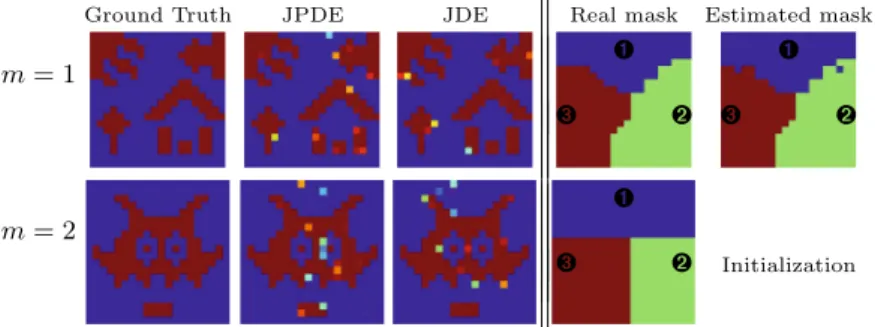
Artificial Datasets.Experiments have been carried out on artificial fMRI data generated according to Eq. (1). We simulated a random mixed sequence of in-dexes coding forM = 2 different stimuli composed of 30 trials each. The resulting ternary sequence was then multiplied by stimulus-dependent and space-varying NRLs, which were drawn from the prior distributionp(A;θa). To this end, 2D slices composed of 20 x 20 binary labelsQm(activating and non-activating vox-els) were constructed for each stimulus type m (see Fig. 1[Left]). Given these labels, the NRLs were simulated as follows, form= 1,2:amj |qmj = 1∼ N(0,0.5) and amj |qmj = 2 ∼ N(3.2,0.5) (see Fig. 2[Left]). As regards HRFs, three groups (K = 3) were considered and spatially organized in three parcels of similar size (labels Z) as shown in Fig. 1[Top-right]. Within each parcel, all voxels share the same HRF prior parameters (¯hk,Σk¯ ). The mean HRF shapes (¯hk)k=1:K are depicted in Fig. 3 and show strong fluctuations across parcels. Diagonal prior covariance matrices ( ¯Σk)k=1:K were considered to draw voxel-specific HRFs according top(hj|zj=k).
As regards parcellation, Fig. 1[Top-right] shows the ability of JPDE to recover the spatial support of hemodynamic territories with high accuracy (1% of misclassified voxels and a DICE index of 0.993) from an imperfect initializa-tion (Fig. 1[Bottom-right]). The HRF variability does not seem to affect the activation maps which are equally well estimated in the JPDE and JDE cases (Fig. 1[Left]). However, a clear difference is seen on the estimated HRFs, which are depicted in Fig. 3 together with the ground truth: the three parcel-specific HRF estimates using JPDE are plotted as well as the single JDE-based HRF time course obtained by merging all parcels. The JPDE estimation is accurate
for all parcels although the parcels cover different proportions of activation areas (i.e.useful signal). In contrast, JDE provides an intermediate HRF shape which lies between those of the three parcels. This explains the observed differences between the two models in terms of estimated NRL dynamics and points out the JDE sensitivity to the choice of thea priori parcellation. When imperfect,
Ground Truth JPDE JDE Real mask Estimated mask
m= 1 ➌ ➋ ➌ ➋ ➊ ➊ m= 2 ➌ ➋ Initialization ➊
Fig. 1. Left: reference activation labels and Posterior Probability Maps (PPM) for JPDE and JDE (a single parcel is assumed for JDE);Right:reference, estimated and initial parcellation masks
Ground Truth JPDE JDE JPDE-JDE
m= 1
m= 2
Fig. 2.Reference and estimated NRLs using JPDE (3 parcels) and JDE (1 parcel)
% Δ B O LD si gn al ¯ h1 h¯2 h¯3
Time (s) Time (s) Time (s)
Fig. 3.Reference and estimated HRF patterns (¯hk) for each parcel using JPDE and JDE
JDE is forced to miss-fit the real HRF shape, and therefore activation dynamics. In the same context, JPDE is able to automatically refine an initial parcellation and provide reliable detection and estimation results.
Interestingly, the NRL differences in Fig. 2 (see the JPDE-JDE plots in Fig. 2[Right]) show that NRL estimates with JPDE have higher pic values, which means that JPDE allows retrieving stronger activation dynamics closer to the ground truth. The most significant NRL differences lie in parcels 2 and 3 where the JDE HRF estimate differs the most from the ground truth. In terms of Mean Square Error (MSE), reported values confirm the performance of JPDE over JDE:M SEm=1 JDE = 0.0182vs M SEm =1 JPDE = 0.0107 and M SEm =2 JDE = 0.0183 vsM SEm=2 JPDE= 0.0141.
Real Data. fMRI data were recorded at 3 T (Siemens Trio) using a gradient-echo EPI sequence(TE=30ms/TR=2.4s/thickness=3mm/FOV=192mm2)during a Localizer experiment [11] with a fast event-related paradigm. The paradigm in-volved sixty auditory (Aud.), visual (Vis.) and motor stimuli, defined in ten experimental conditions (Aud./Vis. sentences, Aud./Vis. calculations, left/right Aud. and Vis. clicks, horizontal and vertical checkerboards). For the considered dataset, the acquisition consisted of a single session of N = 128 scans, yield-ing 3-D volumes with a spatial resolution of 2×2×3mm3. In this experiment, we focus on the Auditorycondition which is supposed to reveal activations in the temporal lobes. The initial parcellation used (from [12]) and the JPDE es-timated one are shown in Fig. 4[Top-middle]. It appears that JPDE groups a number of initial parcels as they turn out to have similar hemodynamic proper-ties, which suggests that the initial parcellation may be unnecessarily too fine. JPDE retrieves respectively three and two different parcels in the left and right temporal regions of interest (ROI). However, JPDE HRF estimates (Fig. 4[Top-right]) show very close shapes for parcels 1 and 3 for the left ROI, which explains
Anatomical superposition
Initial parcels Estimated parcels
JPDE JDE JPDE-JDE
Left ROI
Right ROI
Fig. 4. Left:ROI definition; Middle:Initial and estimated parcels (top), NRL esti-mates with JDE and JPDE and difference image (bottom);Right:HRF estimates for the estimated parcels
the reduced size of the third parcel. As regards activation levels, Fig. 4[Bottom-middle] shows the estimated NRLs using JPDE and JDE. The difference image in Fig. 4 confirms the ability of JPDE to retrieve stronger activations w.r.t. to JDE.
5
Conclusion
We proposed a JPDE framework that provides an automatic parcellation of the brain into homogeneous hemodynamic territories. The quality and reliability of such a parcellation is at the core of robust neural activity detection and brain hemodynamics estimation. By enabling a fully adaptive data-dependent iden-tification of the parcels, the JPDE framework greatly extends the possibilities of detection-estimation approaches. The gain in removing the commitment to a priori fixed territories has been confirmed in preliminary experiments that showed that the JPDE achieved better results than the standard JDE using a fixed parcellation. An important remaining question raised by this new frame-work is related to the issue of choosing the right number of HRF groups at best i.e.in a sparse manner so as to capture the spatial variability in hemodynamic territories while enabling the reproducibility of parcel identification across fMRI datasets. This question should be the most critical to validate our approach but also the most interesting to neuroscientists in case of success. For this specific point, we shall investigate variational approximations of standard information criteria [5] such as the Bayesian Information Criterion.
References
1. Boynton, G.M., Engel, S.A., Glover, G.H., Heeger, D.J.: Linear systems analysis of functional magnetic resonance imaging in human V1. J. Neurosci. 16, 4207–4221 (1996)
2. Celeux, G., Forbes, F., Peyrard, N.: EM procedures using mean field-like approx-imations for Markov model-based image segmentation. Patt. Rec. 36, 131–144 (2003)
3. Chaari, L., Forbes, F., Vincent, T., Dojat, M., Ciuciu, P.: Variational Solution to the Joint Detection Estimation of Brain Activity in fMRI. In: Fichtinger, G., Martel, A., Peters, T. (eds.) MICCAI 2011, Part II. LNCS, vol. 6892, pp. 260–268. Springer, Heidelberg (2011)
4. Ciuciu, P., Poline, J., Marrelec, G., Idier, J., Pallier, C., Benali, H.: Unsupervised robust non-parametric estimation of the hemodynamic response function for any fMRI experiment. IEEE Trans. Med. Imag. 22(10), 1235–1251 (2003)
5. Forbes, F., Peyrard, N.: Hidden Markov Random Field model selection crite-ria based on mean field-like approximations. IEEE Trans. Patt. Anal. Mach. In-tell. 25(9), 1089–1101 (2003)
6. Glover, G.H.: Deconvolution of impulse response in event-related BOLD fMRI. Neuroim. 9, 416–429 (1999)
7. Goutte, C., Nielsen, F., Hansen, L.K.: Modeling the haemodynamic response in fMRI using smooth FIR filters. IEEE Trans. Med. Imag. 19(12), 1188–1201 (2000)
8. Handwerker, D.A., Ollinger, J.M., Mark, D.: Variation of BOLD hemodynamic responses across subjects and brain regions and their effects on statistical analyses. Neuroim. 21, 1639–1651 (2004)
9. Kershaw, J., Ardekani, B.A., Kanno, I.: Application of Bayesian inference to fMRI data analysis. IEEE Trans. Med. Imag. 18(12), 1138–1152 (1999)
10. Makni, S., Idier, J., Vincent, T., Thirion, B., Dehaene-Lambertz, G., Ciuciu, P.: A fully Bayesian approach to the parcel-based detection-estimation of brain activity in fMRI. Neuroim. 41(3), 941–969 (2008)
11. Pinel, P., Thirion, B., M´eriaux, S., Jobert, A., Serres, J., Le Bihan, D., Poline, J.B., Dehaene, S.: Fast reproducible identification and large-scale databasing of individual functional cognitive networks. BMC Neurosci. 8(1), 91 (2007)
12. Thirion, B., Flandin, G., Pinel, P., Roche, A., Ciuciu, P., Poline, J.B.: Dealing with the shortcomings of spatial normalization: Multi-subject parcellation of fMRI datasets. Hum. Brain Mapp. 27(8), 678–693 (2006)
13. Vincent, T., Risser, L., Ciuciu, P.: Spatially adaptive mixture modeling for analysis of within-subject fMRI time series. IEEE Trans. Med. Imag. 29, 1059–1074 (2010) 14. Wager, T.D., Vazquez, A., Hernandez, L., Noll, D.C.: Accounting for nonlinear BOLD effects in fMRI: parameter estimates and a model for prediction in rapid event-related studies. Neuroim. 25(1), 206–218 (2005)
15. Wang, J., Zhu, H., Fan, J., Giovanello, K., Lin, W.: Adaptively and Spatially Estimating the Hemodynamic Response Functions in fMRI. In: Fichtinger, G., Martel, A., Peters, T. (eds.) MICCAI 2011, Part II. LNCS, vol. 6892, pp. 269–276. Springer, Heidelberg (2011)
16. Woolrich, M., Jenkinson, M., Brady, J., Smith, S.: Fully Bayesian spatio-temporal modelling of fMRI data. IEEE Trans. Med. Imag. 23(2), 213–231 (2004)