Sparsity-Promoting Optimal Controller Design

(1)

Lehigh University

Lehigh Preserve

Theses and Dissertations

2018

Sparsity-Promoting Optimal Controller Design

MirSaleh Bahavarnia

Lehigh University

Follow this and additional works at:https://preserve.lehigh.edu/etd Part of theMechanical Engineering Commons

This Dissertation is brought to you for free and open access by Lehigh Preserve. It has been accepted for inclusion in Theses and Dissertations by an authorized administrator of Lehigh Preserve. For more information, please [email protected].

Recommended Citation

Bahavarnia, MirSaleh, "Sparsity-Promoting Optimal Controller Design" (2018).Theses and Dissertations. 4221.

(2)

Sparsity-Promoting Optimal Controller Design

by

MirSaleh Bahavarnia

A Dissertation

Presented to the Graduate and Research Committee of Lehigh University

in Candidacy for the Degree of Doctor of Philosophy

in

Mechanical Engineering

Lehigh University May 2018

(3)

c

(4)

Approved and recommended for acceptance as a dissertation in partial fulfillment of the requirements for the degree of Doctor of Philosophy.

MirSaleh Bahavarnia

Sparsity-Promoting Optimal Controller Design

Date

Prof. Nader Motee, Dissertation Director, Chair

Accepted Date

Committee Members

Prof. Eugenio Schuster

Prof. Subhrajit Bhattacharya

(5)

To My Beloved Mother (Mehrangiz), Father (MirAliakbar), and Sisters (Nasrin and Neda).

(6)

Acknowledgements

First of all, I would like to kindly thank my advisor, Prof. Nader Motee for his inspiring supervisions. Without his fruitful advices, I would not be able to reach insightful understanding of my research interests. He helped me to come out of my comfort zone and search for novel ideas to develop new control theoretic efficient algorithms to reach our fundamental objectives. Definitely, my research path was full of difficulties as others. However, I am proud to say that he greatly supported me through such a path to overcome those difficulties. Particularly, I should be grateful for suggesting the amazing research topic by him. Honestly, I really enjoyed throughout my Ph.D. research activities in such an amazing research area.

I am pleased to express my gratitude to the rest of my Ph.D. committee members including Prof. Eugenio Schuster, Prof. Subhrajit Bhattacharya, and Prof. Frank E. Curtis for their extremely kind supports along my general exam, Ph.D. proposal defense, and Ph.D. dissertation defense. I have learnt so many control concepts from Prof. Schuster through my Ph.D. studies. Prof. Bhattacharya’s motivating comments helped me to strongly deal with research problems. I have been lucky to attend Prof. Curtis’s nonlinear programming class and learn so many effective tools in nonlinear optimization from him. Regarding the academic writing/presentation skills, I should be thankful to Ms. Rita DiFiore-Czipczer and Ms. Teresa Cusumano. I am also thankful to the Department of Mechanical Engineering and Mechanics kind staff including Ms. JoAnn Casciano, Ms. Jennifer Smith, Ms. Barbara McGuire, Mr.

(7)

Muhammed Naazer, and Ms. Allison Marsteller. I am deeply grateful to Prof. Gary Harlow, Prof. John Coulter, and Prof. Donald Rockwell for their kind supports. Let me thank Ms. Bonnie Beidleman, Ms. Jeanne Ma, Ms. Clara Buie, and Ms. Olga Scarpero, for their kind helps at OISS. Additionally, I appreciate my Lehigh University teachers’ kind efforts which facilitated expansion of my knowledge in various fields.

My deep appreciation goes to Prof. Mohammad Saleh Tavazoei who was my B.Sc. advisor and collaborator at Sharif University of Technology. He was the first person who made the control theory interesting for me via his insightful taught control theory courses. Also, I had a chance to start my academic research and publish my first journal paper, first conference papers, and first book chapter along with him. In addition, I should thank Prof. Mohammad Mobed and Prof. Nasser Sadati who taught me the rest of wonderful fundamental control theory courses. Also, I am grateful to all the other teachers from my B.Sc. university, high school, guidance school, and primary school who made me familiar with their fantastic taught courses. Let me take a moment to thank the rest of my collaborators including Dr. Reza Arastoo, Dr. Mayuresh V. Kothare, Mr. Hossein K. Mousavi, Dr. Paulo Tabuada, and Dr. Christoforos Somarakis. Among those, I have been in touch with Dr. Arastoo from 2013 and we have had a great collaborative publications from 2015 till now. I had a chance to collaborate with Mr. Mousavi in one of his specific research areas. He has provided me with interesting ideas through our collaborations. I should deeply appreciate Dr. Tabuada’s comprehensive comments on one of my important research items. Without his fruitful comments, we would not be able to do such a solid research work. My kind thanks go to Dr. Somarakis who presented two of our research papers in CDC 2017. He has provided me with his philosophical thoughts in doing research. I should thank the group of my friends who have supported me along my grad-uate life at Lehigh University: Dr. Milad Siami, Ms. Rozhin Hajian, Dr. Alireza Yektamaram, Dr. Vahid Gholizadeh, Dr. Sadegh Bolouki, Ms. Shokoufeh Elahi,

(8)

Mr. Yousef Jalali, Dr. Omid Ahmadi, Prof. Arash Naraghi, Ms. Maral Adeli, Mr. Nasser Heydari, Ms. Elnaz Rasti, Mr. Yaser Ghaedsharaf, Ms. Shima Dezfulian, Mr. Mohammad Shahabsafa, Ms. Sajedeh Yazdanparast, Dr. Ebrahim Tahmasebi, Dr. Forough Mahmoudabadi, Mr. Afshin Oroojlooy, Ms. Somayeh Khakpash, Mr. Evan Eckersley, Mr. Daniel Beadle, Ms. Maryam Daviran, Ms. Shabnam Ghiasvand, Mr. Mohammad Javad Asadi, Mr. Ali Almasi, Mr. Daniel Loikits, Mr. Kuanchen Xiong, Mr. Nasser Vahedi, Mr. Vahid Rahmanian, Mr. Alireza Famili, Mr. Majid Jahani, Mr. Mohammad Pirhooshyaran, Mr. Soheil Sadeghi, Mr. Pedram Yousefian, Mr. Saleh Teymouri, Mr. Arash Amini, and Mr. Milad Habibi.

It is a great honor for me to thank my artist friends who helped me to tolerate the difficulties of Ph.D. studying away from my home country via their awesome artistic works: Mr. Mohammad Haghighi, Mr. Mahdi Ghorbaniantabrizi, Mr. Mostafa Saffarian, Mr. Nariman Hodjati, Mr. Mostafa Jafari, Mr. Abbas Jamshidi, Mr. Behzad Shaghaghi, Ms. Masoumeh Radjabi, Mr. Shayan Keshavarz, Mr. Alireza Shahmohammadi, Mr. Omid Sayareh, Mr. Faraz Minooei, Ms. Sepideh Raissadat, Mr. Iman Vaziri, Mr. Amir Khajehpour, Ms. Hanna Davarmanesh, Dr. Reza Rezaiesarlak, Mr. Sirvan Manhoobi, Mr. Behfar Bahadoran, and Ms. Shabnam Ahangar.

I should also thank some of my old friends from my either high school or B.Sc. degree university: Mr. Salar Jarhan, Mr. Reza Salemmilani, Mr. Saeed Saeedmonir, Mr. Yahya Alamdarimilani, Dr. Sadra Sadraddini, Dr. Alborz Alavian, Ms. Hadis Mohammadi, Mr. Salar Fattahi, Mr. Hesam Mohammadi, Ms. Sepideh Hasan-moghadam, Mr. Reza Khodaeimehr, Mr. Amirhossein Taghvaei, and Dr. Armin Zare.

(9)

List of Tables

2.1 Parameters for mass-spring system. . . 31 2.2 Parameters for synchronous generators with sparse interconnection topology. 34 2.3 Parameters for network with unstable nodes. . . 36

3.1 Matrix operators . . . 48

4.1 Power parameters used in our numerical simulations. . . 96 4.2 Performance and cardinality quantities for the case ρrel∈ {0 %,30 %}. . . 96

7.1 Cost and cardinality quantities for F (LQR) and Fnf s (NFS) (10,000×

10,000 randomly generated system). . . 146 7.2 Cost and cardinality quantities for F (LQR) and Fnf s (NFS) (10,000×

10,000 sub-exponentially spatially-decaying system). . . 149 7.3 Relative performance/sparsity specifications for closed loops withF (LQR)

and Fnf s _{(NFS) (130}_×_{130 IEEE 39-bus New England power system).} _{. .} ₁₅₂

7.4 Cost and cardinality quantities forF (Sparse LQR) andFnf s (NFS) (100×

100 randomly generated system).. . . 155

8.1 Dependency of quantitiesRF,Ru, and Don parameterα.. . . 191

9.1 Performance/Sparsity quantities for K and KT in the case of 10×10 ran-domly generated system J(F) = 151.2711 andkFk0 = 100

(17)

9.2 Performance quantities for fixed values of sparsity quantities aroundσD =

40 and varying values ofq. (For the 100×100 randomly generated system). 215 9.3 Performance quantities for fixed values of sparsity quantities aroundσD =

60 and varying values ofq. (For the 100×100 randomly generated system). 216 9.4 Performance quantities for fixed values of sparsity quantities aroundσD =

80 and varying values ofq. (For the 100×100 randomly generated system). 217 9.5 Performance/Sparsity quantities forK in the case of 10,000×10,000

ran-domly generated system J(F) = 3.5302×106 and kFk0 = 108

. . . 218 9.6 Performance/Sparsity quantities forK in the case of 10,000×10,000

sub-exponentially spatially decaying system J(F) = 8.4077×105 and kFk₀ = 108

. . . 220 9.7 Performance/Sparsity quantities for ˆLin the case of 1,000×1,000 randomly

generated undirected network J(L) = 0.4993 andkAk0= 999,000

(18)

List of Figures

2.1 Density-Performance trade-off curves for a mass-spring system (C2 =

I) (a)RJ percentage versusRD (b)R2 percentage versusRD

percent-age (c)R∞ percentage versusRD percentage. . . 38

2.2 Density-Performance trade-off curves for a mass-spring system (C2 6=

I) (a)RJ percentage versusRD (b)R2 percentage versusRD

percent-age (c)R∞ percentage versusRD percentage. . . 39

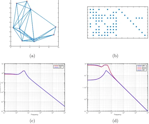
2.3 State feedback (C2 = I): (a) Spatial distribution of sparse intercon-nection topology consisting of 10 synchronous generators. Blue solid lines represent the bi-directional links connecting synchronous genera-tors specified by red ∗(b) The sparsity pattern of sparsified controller

K. Blue dots represent the non-zero elements (c) Schatten 2-norm of

S (Red) and ˆS (Blue) (d) Maximum/minimum singular values of S

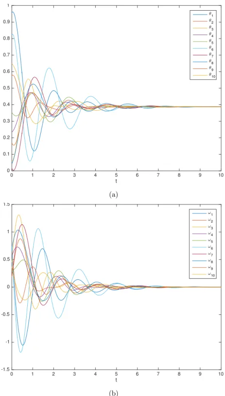
(Red) and ˆS (Blue). . . 40 2.4 State feedback (C2 =I): (a) Angles versus time (b) Angular velocities

(19)

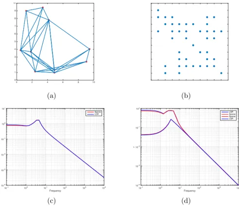
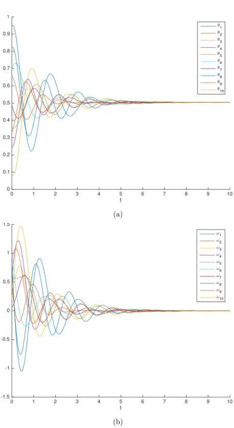
2.5 Structured state feedback (C2 6= I): (a) Spatial distribution of sparse interconnection topology consisting of 10 synchronous generators. Blue solid lines represent the bi-directional links connecting synchronous generators specified by red ∗ (b) The sparsity pattern of sparsified controllerK. Blue dots represent the non-zero elements (c) Schatten 2-norm ofS (Red) and ˆS (Blue) (d) Maximum/minimum singular values of S (Red) and ˆS (Blue). . . 42 2.6 Structured state feedback (C2 6=I): (a) Angles versus time (b) Angular

velocities versus time. . . 43 2.7 Spatial distribution of 15 unstable nodes and the sparsity visualization

of sparsified controller K. Blue solid lines, red dashed lines, blue ◦, and black∗, represent the bi-directional links, one-way links, self-loops, and no-self-loops, respectively. . . 44 2.8 Spatial distribution of 15 unstable nodes and the sparsity visualization

of sparsified output feedback controllerK. Blue solid lines, red dashed lines, blue ◦, and black ∗, represent the bi-directional links, one-way links, self-loops, and no-self-loops, respectively. . . 44

3.1 IEEE 39-bus power system model . . . 64 3.2 Performance loss percentage versus spatio-temporal sparsity criterion

per-centage forδ = 0.1 andδ = 0.2 (IEEE 39-bus power network). . . 65 3.3 Sparsity pattern of designed controller for δ = 0.2 and γ = 10−1 (IEEE

39-bus power network). The corresponding performance loss percentage is equal to 6.8862 %. Blue dots represent the non-zero elements. . . 65 3.4 Performance loss percentage versus spatio-temporal sparsity criterion

(20)

3.5 Sparsity pattern of designed controller for δ = 0.2 and γ = 10−5 (10×10 randomly-generated system). The corresponding performance loss percent-age is equal to 79.0340 %. Blue dots represent the non-zero elements. . . . 66 3.6 Performance loss percentage versus spatio-temporal sparsity criterion

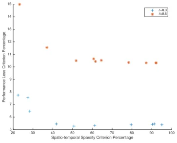
per-centage forδ = 0.3 andδ = 0.6 (10×10 spatially-decaying system). . . 67 3.7 Sparsity pattern of designed controller forδ = 0.6 andγ = 0.00001 (10×10

spatially-decaying system). The corresponding performance loss percentage is equal to 14.9894 %. Blue dots represent the non-zero elements. . . 68

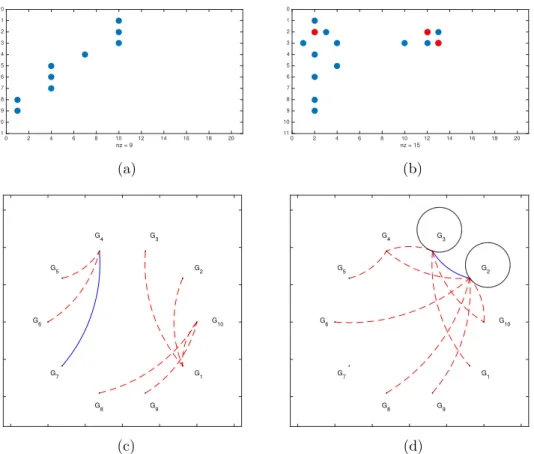
4.1 IEEE 39-bus power system model . . . 88 4.2 (a) Sparsity pattern of K for ρrel = 0%; Blue and red bullets are used to

depict diagonal and off-diagonal elements of K, respectively (b) Sparsity pattern ofK forρrel= 30% (i1, i2) = (2,3)

. Blue and red dots represent the off-diagonal and diagonal non-zero elements, respectively. (c) Sparsity graph of |Kθ|+|Kω| forρrel = 0%; Blue solid lines, red dashed lines, and

black self-loops are used to depict doubly-connected, singly-connected, and self-connected edges of|Kθ|+|Kω|, respectively (d) Sparsity graph of|Kθ|+

|K_ω|forρrel= 30% (i1, i2) = (2,3)

. . . 90 4.3 Gray scale pattern of susceptance of all links of power network, i.e.,L. . . 92 4.4 (a) Gray scale pattern of f(Kθ) +f(Kω) for ρrel = 30 % (b) Gray scale

pattern of f(|K_θ|+|Kω|) for ρrel= 30 %. . . 94

4.5 (a)f(Kθ) +f(Kω) versusρrel % (b) f(|Kθ|+|Kω|) versusρrel %. . . 97

4.6 Frequency characteristics of the closed loop systems controlled by the LQR (blue), the sparse controller (red) for the case ρrel = 0 %, and the sparse

controller (green) for the case ρrel = 30 %. (a) and (b) depict maximum

and minimum singular values for the cases of ρrel = 0 % and ρrel = 30 %,

respectively. (c) and (d) exhibit the Schatten 2-norm of the closed loop system (c) case ρrel= 0 % (d) case ρrel= 30 %

(21)

5.1 Positions ofN = 10 randomly generated nodes in a 10×10 box-shape region.111 5.2 (a) Sparsity visualization ofK forτ = 0 (b) Sparsity visualization ofK for

τ = 9. Blue dots represent the non-zero elements. . . 113 5.3 (a) Cardinality percentage versusτ (b) Performance loss percentage versusτ.115 5.4 Performance-Sparsity trade-off for different values of 6 uniformly selected

time-delay τ and 20 logarithmically spaced sparsity-promoting parameter

γ ∈[10−4,10−1]. . . 116

6.1 Sparsity pattern of row-column (10,13)-sparse LQC design for 25× 25 randomly-generated system with 25×20 randomly-generated input matrix

B. Blue dots represent the non-zero elements and it nz denotes the number of non-zero elements. . . 130 6.2 Relationship between r and R % for 25 ×25 randomly-generated system

with 25×20 randomly-generated input matrix B. . . 131 6.3 Relationship between c and R % for 25×25 randomly-generated system

with 25×20 randomly-generated input matrix B. . . 132

7.1 Eigenvalues of open loop and closed loop for F (LQR) (10,000×10,000 randomly generated system). . . 146 7.2 Eigenvalues of open loop and closed loop forFnf s (NFS) (10,000×10,000

randomly generated system). . . 147 7.3 Eigenvalues of open loop and closed loop forF (LQR) (10,000×10,000

sub-exponentially spatially-decaying system). . . 148 7.4 Eigenvalues of open loop and closed loop for Fnf s _{(NFS) (10}_,₀₀₀_×

(22)

7.5 Sparsity pattern ofFnf s(NFS); Each blue spot represents a nonzero element of the state feedback controller and number of nonzero elements of the state feedback controller is denoted by nz (10,000×10,000 sub-exponentially spatially-decaying system). . . 150 7.6 Sparsity pattern of first 1,000×1,000 diagonal sub-block of Fnf s (NFS);

Each blue spot represents a nonzero element of the state feedback controller and number of nonzero elements of the state feedback controller is denoted bynz (10,000×10,000 sub-exponentially spatially-decaying system). . . . 151 7.7 Sparsity pattern ofFnf s_{(NFS); Each blue spot represents a nonzero element}

of the state feedback controller and number of nonzero elements of the state feedback controller is denoted bynz(130×130 IEEE 39-bus New England power system). . . 152 7.8 Sparsity pattern ofFnf s(NFS); Each blue spot represents a nonzero element

of the state feedback controller and number of nonzero elements of the state feedback controller is denoted bynz(100×100 randomly generated system).153 7.9 Sparsity pattern of F (Sparse LQR); Each blue spot represents a nonzero

element of the state feedback controller and number of nonzero elements of the state feedback controller is denoted bynz(100×100 randomly generated system). . . 154 7.10 The trade-off between upper bound on non-fragility and sparsity level for

Sparse LQRs F designed by [1] (Blue) and Fnf s (NFS) (Red) (100×100 randomly generated system). . . 156 7.11 The visualization of σP (%) versus σD (%) obtained from brute force

greedy algorithm (15×15 randomly generated system). . . 158 7.12 The visualization of σP (%) versus σD (%) obtained from brute force

and gradient-based greedy algorithms (20× 20 randomly generated system). . . 161

(23)

8.1 A non-convexity in the nature of constraint of (P3) in terms of form of dependency on argumentξ. . . 176 8.2 Positions ofN = 10 randomly generated nodes in a 10×10 box-shape region.188 8.3 (a) Relative cardinality of controllers 100×(kF_kk₀/kF_LQRk₀) versus

trigger-ing timestk(b) Relative cardinality of control inputs 100×(kukk0/kuLQRk k0) versus triggering timestk. . . 194

8.4 (a) The Euclidean norm of state trajectories of SSOC and periodic time-triggered LQR designkxkk2 versus triggering timestk (b) State trajectories

x(i)_{’s of SSOC starting from an arbitrarily-chosen}_x

0 fori∈ {1,2,· · · ,19,20}.195 8.5 Inter-Execution times δk versus time t. . . 196

8.6 (a) Average relative cardinality of controllers RF versus spatially decaying

rateβ. (b) Average relative cardinality of control inputsRuversus spatially

decaying rate β. . . 197 8.7 Average inter-execution timeD versus spatially decaying rateβ. . . 198 8.8 (a) Average relative cardinality of controllersRF versus penalizing

parame-terγ. (b) Average relative cardinality of control inputsRu versus penalizing

parameterη. . . 199

9.1 Geometrical visualization of 3 possible cases (γ = 1.1γij > γij, γ = γij, or

γ = 0.9γij < γij) in which function g attains 1, 2, or 3 roots, respectively,

in the case ofFij = 4 and q= 0.4. . . 210

9.2 Plots of function g in 3 possible cases (γ = 1.1γij > γij, γ = γij, or γ =

0.9γij < γij) in the case of Fij = 4 andq = 0.4. . . 211

9.3 Plots of functionsh3,h4, and the corresponding tangent line to functionh4 in the case ofγ =γij = 4.8330, Fij = 4, andq = 0.4. . . 212

(24)

9.4 Sparsity-Performance trade-off curves for varying values ofq. We set the fol-lowing visualization rules: (i) qRed_{< q}Green _{< q}Blue _(ii) _qCircle _{< q}Asterisk _<

qPlus,wherein each superscript refers to the corresponding color or sign as-sociated withq. (For the 100×100 randomly generated system). . . 215 9.5 Sparsity-Performance trade-off curves aroundσD = 40 for varying values of

q. We set the following visualization rules: (i) qRed < qGreen < qBlue (ii)

qCircle< qAsterisk< qPlus,wherein each superscript refers to the correspond-ing color or sign associated withq. (For the 100×100 randomly generated system). . . 216 9.6 Sparsity-Performance trade-off curves aroundσD = 60 for varying values of

qCircle< qAsterisk< qPlus,wherein each superscript refers to the correspond-ing color or sign associated withq. (For the 100×100 randomly generated system). . . 217 9.7 Sparsity-Performance trade-off curves aroundσD = 80 for varying values of

qCircle< qAsterisk< qPlus,wherein each superscript refers to the correspond-ing color or sign associated withq. (For the 100×100 randomly generated system). . . 218 9.8 Sparsity pattern of the first 100×100 sub-block ofK in the case of 10,000×

10,000 randomly generated system (Blue dots represent the non-zero el-ements and ”nz” denotes the number of non-zero elel-ements of the first 100×100 sub-block of K). . . 219 9.9 Sparsity pattern of K in the case of 10,000×10,000 sub-exponentially

spatially decaying system (Blue dots represent the non-zero elements and ”nz” denotes the number of non-zero elements ofK). . . 220

(25)

9.10 (a) Graph representation of subgraph consisting of the first 50 nodes of L

and its corresponding links (b) Graph representation of subgraph consisting of the first 50 nodes of ˆLand its corresponding links. (For the 1,000×1,000 randomly generated undirected network). . . 223

(26)

Abstract

Considering the class of linear time-invariant (LTI) systems and utilizing the vari-ous mathematical tools, for diverse scenarios, we design sparsity-promoting feedback controllers while attaining a reasonable performance loss. Diverse scenarios can be classified as follows: (i) feedback controller sparsification subject to attain a simi-lar frequency behavior for the case without/with parametric uncertainty (Chapters 2 and 4) (ii) improvement on sparsity in time domain in addition to sparsity promotion in feedback controller (Chapters 3 and 8) (iii) sparse feedback controller design for uncertain time-delay systems (Chapter 5) (iv) row-column (r, c)-sparse feedback con-troller design (Chapter 6) (v) feedback concon-troller sparsification for large-scale systems (Chapters 7 and 9). Sparsity promotion in feedback controller is done via several tech-niques including `1-relaxation, a notion of non-fragility, and quasi-norms. Sparsity improvement in time domain is obtained via periodic time-triggered and self-triggered control. In Chapters 2, 3, 4, 5, and 6, the non-convexity arisen by Lyapunov stability condition is handled utilizing the bi-linear rank penalty technique. In Chapters 7 and 9, stability is provided by means of continuity of maximum real part of eigenvalue of the closed-loop system. In Chapter 8, stability is imposed by a performance-based condition which consists of a quadratic cost-to-go and a Lyapunov function.

(27)

Chapter 1 Introduction

1.1 Literature Review

The area of sparsity-promoting control systems has been growing rapidly in the past decade and it has been applied to various real-world applications such as formation control of autonomous vehicles, frequency synchronization in wide area control of power networks, transportation networks, mobile wireless networks, only to name a few. In several important applications, the centralized control methodologies are unable to be applied due to the lack of access to global information in subsystem level throughout the network. Such a design constraint has motivated researchers to investigate the possibility of designing near-optimal sparse feedback controllers for large-scale dynamical networks [1–35].

To generally solve the sparsity-promoting control problems, diverse methods have been proposed. In [1, 6], the authors propose an ADMM-based primal-dual itera-tive approach which also takes advantage of conjugate gradient method. In [36], a projection-based method is developed in which some bounds on the optimal value of the sparsity-constrained problem is presented. Motivated by linearization idea, utilizing the sequential convex programming has led to the methods proposed by

(28)

[18, 20].

All the methods mentioned so far (except the [18]), have been proposed for the continuous-time setup. However, in addition, some methods have been presented by considering the discrete-time setup which propose sparsity-promoting state feedback gain controllers [13, 18, 37–40]. In [38, 39], a decentralized state feedback controller is presented based on convex relaxations where utilizing a graph theoretic proof, an upper bound on rank of the relaxed SDP solution is derived and if such a rank is equal to 1, then the globally optimal solution can be reconstructed from the relaxed SDP solution. However, the solution obtained by such a relaxation-based method is decentralized and is not presented for general sparse controllers. But, it is spanning both finite and infinite horizon discrete-time sparsity-promoting LQR problems.

The methods presented in [13, 22] are basically classified as (convex optimization)-based methods. Another recently proposed method recast the sparsity-promoting optimal control problem as a rank-constrained optimization problem, then tries to take advantage of ADMM and Singular Value Decomposition (SVD) to deal with such a rank-constrained optimization problem [21]. Authors in [27, 28, 32, 35], in-stead of utilizing ADMM, have utilized bi-linear rank penalty technique to tackle the rank-constrained optimization problem. The solution proposed by such a technique, satisfies a rank inequality which features the sub-optimality of the proposed solu-tion. Newly, in [33], the authors have novelly proposed a non-fragility based method for sparsification of large-scale feedback controllers. Also, another large-scale feed-back controller sparsification is proposed by [41] which is built upon minimization of quasi-norms.

One of the newly-investigated systems in sparsity-promoting control is spatially decaying systems [7, 14, 30, 42]. In such research works, a large class of spatially decaying systems is classified where their quadratically-optimal feedback controllers inherit spatial decay property from the dynamics of the underlying system. Moreover,

(29)

a method based onq-Banach algebras is proposed where sparsity and spatial localiza-tion features of spatially decaying systems can be studied whenq is chosen sufficiently small or sufficiently large. For the class of spatially distributed systems, due to specific properties of such systems, truncation-based theoretical sparsity-promoting optimal control designs are provided by [30, 42]. Obviously, for a general class of systems, it is not possible to derive and design theoretical sparsity-promoting controllers.

The concept of sparsity is not limited to the space of state feedback controllers. In other words, the concept of sparsity can be considered in the time domain as well. To be more specific, time-triggered, self-triggered, or event-triggered methods can be seen as methods in which sparsity in time is promoted in the sense that number of triggering times is supposed to be as few as possible. To address the research works in such an area, we suggest to take a look at [26, 34, 43–65].

1.2 Main Contributions

1.2.1 Dense Output Feedback Controller Sparsification while

Preserving its Frequency Characteristics

The dense output feedback controller sparsification is investigated while the frequency characteristics of designed closed-loop system remains similar to that of the system controlled with dense one. Considering a well-performing pre-designed dense con-troller and utilizing the concept of H2/H∞ control, a rank constrained optimization problem is developed which has the capability of transferring such a dense controller to a sparse one while preserving the frequency characteristics with reasonable toler-ance. In our proposed method, sparsification leads to less number of communication links and H2/H∞ minimization guarantees the preservation of frequency character-istics. Finally, the effectiveness of our proposed method is evaluated by testing it on synchronous generators with sparse interconnection topology, network with unstable

(30)

nodes, and mass-spring system.

1.2.2 Periodic Time-Triggered Sparse Linear Quadratic

Con-troller Design

The periodic time-triggered sparse Linear Quadratic Controller (LQC) design is in-vestigated for the class of Linear Time Invariant (LTI) systems. Given a time period and keeping the control input fixed during such a time period, an optimization prob-lem is formulated in which the objective function consists of a quadratic performance term along with an `0-regularization term. Recasting such an optimization problem as a rank-constrained optimization problem and utilizing the weighted `1-relaxation enable us to apply so-called bi-linear rank penalty technique to design periodic time-triggered sparse LQC. Employing the various test cases and running our proposed algorithm for different values of time period, performance/sparsity trade-off curves are visualized which suggest a helpful criterion to choose the time period in a way that the desired balance between controller sparsity and rate of periodic triggering is made.

1.2.3 Feedback Controller Sparsification Under Parametric

Uncertainties

We consider the problem of output feedback controller sparsification for systems with parametric uncertainties. The performance of a centralized controller deteriorates as a result of the sparsification process. We develop an optimization scheme that minimizes this deterioration, while promoting sparsity pattern of the feedback gain. In order to improve temporal proximity of an existing closed-loop system and its sparsified counterpart, we also incorporate an additional constraint into the problem

(31)

formulation so as to bound the variation in the system output pre and post spar-sification. We also show that the resulting non-convex optimization problem can equivalently be reformulated into a rank-constrained optimization problem. We then formulate a minimization problem along with an algorithm to obtain a sub-optimal solution via the bi-linear rank penalty technique. Finally, a sub-optimal sparse con-troller design for IEEE 39-bus New England power network is utilized to showcase the effectiveness of our proposed method.

1.2.4 Sparse Memoryless LQR Design for Uncertain Linear

Time-Delay Systems

The sparse memoryless LQR design problem is formulated for uncertain linear time-delay systems. In such a problem, the goal is to minimize a quadratic cost supple-mented by sparsity-promoting term (weighted-`1 in our case) subject to stability of closed-loop system under norm-bounded uncertainty. It is shown that such an op-timization problem can be reformulated as a rank-constrained opop-timization problem which consists of convex constraints except one rank constraint. Utilizing the bi-linear rank penalty technique, the sparse memoryless LQR is designed. Numerous numeri-cal results depict that there exists a trade-off between time-delay and sparsification quality. In addition, the larger time-delay, the poorer performance-sparsity trade-off is observed.

1.2.5 Row-Column Sparse Linear Quadratic Controller

De-sign via Bi-Linear Rank Penalty Technique and

Non-Fragility Notion

We consider the problem of row-column sparse linear quadratic controller (LQC) design. An optimization problem is formulated in which the quadratic performance

(32)

loss is minimized subject to satisfaction of m+n sparsity constraints to obtain the row-column (r, c)-sparse LQC design where m and n refer to the number of inputs and states, respectively andr/crepresent the maximum allowed density level for each row/column of controller. It is expressed that the obtained non-convex optimization problem can equivalently be reformulated as a rank-constrained problem withm+n+1 rank constraints. After applying the non-fragility notion provided by [33] to such a rank-constrained problem, bi-linear rank penalty technique is deployed to find a sub-optimal row-column (r, c)-sparse LQC design which fulfills the rank constraint with desired tolerance. At last, to verify our proposed algorithm, given a randomly generated system, a sub-optimal row-column (r, c)-sparse LQC design is proposed and subsequently, the fundamental trade-off between r/cand quadratic performance loss is visualized.

1.2.6 State Feedback Controller Sparsification via Non-Fragility

Notion

We introduce a notion of non-fragility for a state feedback controller which stabilizes a linear time-invariant (LTI) system. The lower and upper bounds on such an intro-duced non-fragility are derived. On the basis of such derived bounds on non-fragility, a sparsification procedure is developed to obtain sparsified state feedback controllers out of a given stabilizing state feedback controller. Investigating the extensive numer-ical simulations, it is observed that the proposed method is capable of being applied to large-scale systems consisting of thousands of states. As further, as illustrated via case studies, the (non-fragilty)-based sparsification procedure can outperform a well-respected existing method in the literature, in terms of sparsity-performance trade-off behavior. Also, considering a set of sparse stabilizing state feedback controllers and applying the (non-fragilty)-based sparsification procedure, a trade-off between upper

(33)

bound on non-fragility and sparsity level of such state feedback controllers is visual-ized. Moreover, two greedy algorithms are proposed to obtain a set of sparse state feedback controllers out of a given stabilizing state feedback controller.

1.2.7 Improving Sparsity in Time and Space via Self-Triggered

Sparse Optimal Controllers

The optimal control of linear time-invariant (LTI) systems via self-triggered sparse optimal control (SSOC) laws is considered. The control objective is to design an optimal control law which stabilizes the LTI system for all initial conditions, re-quires less sensing, minimizes communication requirements among the subsystems, minimizes the number of active actuators, and provides guaranteed closed-loop per-formance bounds. To achieve such control objectives, a sequence of `0-regularized linear-quadratic optimal control problems is formulated, wherein the objective is to optimize a cost function which involves three terms: one for maximizing the inter-execution time, another for minimizing the number of nonzero elements of the state feedback gain, and the last for minimizing the number of active actuators. Deriving the lower bounds on inter-execution times, we propose a scheme to solve this prob-lem. Such a scheme consists of two main levels: (i) A nonlinear optimization is solved for inter-execution time while the feedback gain is kept fixed. (ii) An `1-relaxed semi-definite program (SDP) is solved for feedback gain while the inter-execution time is kept fixed. We show that the proposed SSOC laws are feasible and results in a stabilizing sequence of sparse optimal controllers. Additionally, we prove that the performance of the resulting closed-loop system does not exceed a pre-specified performance bound. Due to numerical verification of our proposed method on spa-tially distributed systems, the sparsity in time and space is improved compared to the periodic time-triggered LQR design. Moreover, a tradeoff between pre-specified performance bound and sparsity in time/space is observed. Furthermore, the effect

(34)

of spatially decaying rate on sparsification process is visualized.

1.2.8 Feedback Controller Sparsification via Quasi-Norms

We utilize the q ∈ (0,1) quasi-norms to sparsify a given well-performing feedback controller which stabilizes a linear time-invariant (LTI) system. To achieve such a goal, we firstly formulate an unconstrained optimization problem which incorporates two terms: (i) The Frobenius norm of difference of the given feedback controller and the one to be designed; (ii) The q ∈ (0,1) quasi-norm of the feedback controller to be designed. The former term heuristically features the closed-loop stability and the latter term promotes the sparsity. Next, obtaining an analytic threshold for the sparsity-promoting parameter, the analytic solution of the formulated unconstrained optimization problem is expressed which is basically the designed sparse feedback controller. Throughout the numerical simulations, it is observed that in some cases, our proposed method can outperform the well-known truncation operator which ap-pears in cardinality minimization problems. In other words, sometimes, theq∈(0,1) quasi-norms can be more effective than `0 sparsity measure. As another observa-tion, when q decreases, the sparsity-performance balance is significantly improved. Furthermore, our proposed method is interestingly capable of being applied to the large-scale systems with thousands of states.

1.3 Subject-Based Classification of Chapters

1.3.1 Spatial Sparsity

(35)

1.3.2 Temporal Sparsity

Chapters 3 and 8.

1.3.3 Regulation

Chapters 3, 5, 6, and 8.

1.3.4 Disturbance Attenuation

Chapters 2, 4, 7, and 9.

1.3.5 Similar Frequency Behavior

Chapters 2 and 4.

1.3.6 Quadratic Performance Loss Minimization

Chapters 2, 3, 4, 5, 6, and 8.

1.3.7 Design Under Parametric Uncertainty

Chapters 4 and 5.

1.3.8 Design for Time-Delay Systems

Chapter 5.

1.3.9 Feedback Sparsification

(36)

1.3.10 Sparse Feedback Design

Chapters 3, 5, and 6.

1.3.11 State Feedback

Chapters 2, 3, 4, 5, 6, 7, 8, and 9.

1.3.12 Output Feedback

Chapters 2, 4, and 9.

1.3.13 Bi-Linear Rank Penalty Technique

Chapters 2, 3, 4, 5, and 6.

1.3.14 Row-Column Sparsity

Chapter 6.

1.3.15 Non-Fragility

Chapters 6 and 7.

1.3.16 Quasi-Norm Minimization

Chapter 9.

1.3.17 `

1

Relaxation

Chapters 2 , 3, 4, 5, and 8.

(37)

1.3.18 H

2

Minimization

Chapters 2, 3, 4, 5, and 6.

1.3.19 H

∞

Minimization

Chapters 2 and 4.

1.3.20 Convex Optimization Techniques

Chapters 2, 3, 4, 5, 6, and 8.

1.3.21 Non-Convex Optimization Techniques

(38)

Chapter 2 Dense Output Feedback Controller

Sparsification while Preserving its

Frequency Characteristics

2.1 Introduction

Although numerous works have been done in the area of distributed controller design [42, 66] , the capability of efficiently solving the general problem via a systematic approach is far away from the desirable point. For some classes of systems such as spatially invariant systems and spatially decaying systems useful results on the structure of the solution space have been derived [42, 67]. Furthermore, several other design frameworks, each with their specific imperfections, have also been proposed to design sparse/structured controllers for the continuous/discrete time linear time invariant systems both in time and frequency domain [2, 18, 19, 21, 27, 28, 39, 40, 68]. The common approach in the synthesis of distributed controllers is to minimize performance loss subject to stability guarantee and minimization of number of needed communication links among controller nodes. Unlike such an approach and similar to

(39)

methodology presented by [21, 27, 40], our proposed framework in this chapter is based on the assumption that there already exists a well-performing dense controller such as conventional centralized LQR method. We aim to synthesize a sparse controller which preserves the performance characteristics as much as possible close to that of the pre-assumed dense controller. Such a performance preservation is achieved via adopting the concepts from mixedH2/H∞ control [69–71] to not only obtain minimum gap in the frequency characteristics of the closed-loop transfer functions, but also consider the difference between the characteristics of the control signals generated by both dense and sparse controllers.

In particular, firstly, it is assumed a well-performing pre-designed output feed-back controller is given and then considering the bounds on difference of output and control input signals and their corresponding well-performing pre-designed signals, (i.e., H∞-norm of difference between closed-loop constructed by our proposed output feedback controller and the one constructed by such a well-performing pre-designed output feedback controller), respectively, the H2-norm of difference between closed-loop constructed by our proposed output feedback controller and the one constructed by such a well-performing pre-designed output feedback controller is minimized while minimizing the number of communication links of our proposed output feedback con-troller.

It is shown that our proposed synthesis framework can equivalently be reformu-lated as a fixed rank-constrained optimization where all non-convexities are collected into a rank constraint.

This chapter is organized as follows: After expressing our used mathematical notations in Section 2.2, Section 2.3 is dedicated to formulate the problem which is supposed to be solved. In Section 2.4, it is explained how our formulated problem can equivalently be reformulated as an optimization problem consisting of several linear matrix inequalities and a rank constraint. Section 2.5 provides some visions to our

(40)

chosen sparsity measure and the bi-linear rank penalty technique algorithm which is chosen to come up with the corresponding rank-constrained optimization problem. Our sparsification method is verified via various numerical simulations presented in Section 2.6. Finally, Section 2.7 reveals some discussions and conclusions.

2.2 Mathematical Notations

Throughout the chapter, the following notations are adopted: The space of n by

m matrices with real elements is indicated by _Rn×m_{. The} _n _by _n _{identity matrix}

is denoted by In. Operators Tr(.) and rank(.) denote the trace and rank of the

matrix operands. The transpose operator is denoted by (.)T. The matrix element-wise product, i.e., Hadamard product is represented by ◦. A matrix is said to be Hurwitz if all its eigenvalues lie in the open left half of the complex plane. k.k0 represents the cardinality of a vector/matrix, whilek.k1,k.k2, andk.kF denote`1, `2, and Frobenius norm operators, respectively. Also, the norm k.kL2(Rn) is defined by

kxk2_L₂₍_Rn₎:= Z ∞ 0 kx(t)k2 2 dt.

A real symmetric matrix is said to be positive definite (semi-definite) if all its eigen-values are positive (non-negative). _Sn

++ (Sn+) denotes the space of positive definite (positive semi-definite) real symmetric matrices, and the notation X Y (X Y) means X −Y ∈ _Sn

++ (X −Y ∈ Sn+). The ith largest singular value of a matrix is denoted by σi(.).

(41)

2.3 Problem Formulation

Let a linear time invariant (LTI) continuous-time system be given by its state space realization      ˙ x(t) = Ax(t) +B1u(t) +B2d(t) y(t) =C1x(t) , whereA∈_Rn×n_, _B

1 ∈Rn×m, B2 ∈Rn×r, andC1 ∈Rp×n. It is assumed that the pair (A, B1) is controllable and (A, C1) is detectable.

Our goal is to design a static feedback controller

u(t) =KC2x(t), K ∈ K, C2 ∈Rq×n,

which achieves minimum performance difference comparing to a reference well-performing pre-designed dense controller, namely ˆK, while minimizing the number of non-zero elements of the controller matrix. We, also, desire that controller to be contained in a set of admissible feedback gains with previously specified structure, denoted by

K. In this chapter, we just consider the case where the set K is convex, since it reduces the complexity of the problem, and, more importantly, it covers a wide range of practical constraints on the controller that should be considered in the synthesis of the controller. For instance, in some real-world applications, it is not practically feasible to construct a link between special nodes; such limitations are translated to the convex constraints for which the corresponding element of the controller matrix should be equal to zero which can be applied via element-wise Hadamard product. Other practical limitations such as upper bounds on the elements of the controller matrix, (e.g., technological impositions), can also be addressed by convex constraints on controller matrix K.

(42)

by the designed sparse controller, to be in the close neighbourhood of that of the input/output, produced by the original dense controller when an input signal d(t) with bounded energy is applied to the loop plant. Representing the closed-loop systems controlled by the controllers K and ˆK by the state space realizations

S and ˆS, respectively, the search for sparse controller K can be formulated as the following optimization problem:

minimize K,0,1 0+λ11+λ2kKk0 (2.1a) subject to: K ∈ K, (2.1b) A+B1KC2 : Hurwitz, (2.1c) kS −Skˆ 2 H2 ≤0, (2.1d) kyS−ySˆkL2(Rp) < 1kdkL2(Rr), (2.1e)

where k.kH2 and k.kH∞ are H2 and H∞ norms, respectively, and λ1 and λ2 are

reg-ularization parameters. Moreover, positive constants 0 and 1 are upper bounds on

H2 and H∞ norms of difference systemS −Sˆ.

Remark 1. In case of C2 = C1 6= I, the controller K would be an output feedback

controller.

It is worth noting that the term appeared on left hand side of inequality (2.1d) can be simplified into the H2 norm squared of an augmented system, namely ¯S, constructed by the following state space realization matrices:

¯ A=    A+B1KC2 0 0 A+B1KCˆ 2   , ¯ B = B₂T B₂T T , C¯ = C1 −C1 .

Furthermore, the constraint (2.1e) can equivalently be cast by enforcing bounds on the H∞ norm of the closed-loop transfer functions from d(t) to y(t). Then, problem

(43)

(2.1) can be reformulated as follows: minimize K,0,1 0+λ11+λ2kKk0 (2.2) subject to: K ∈ K, A+B1KC2 : Hurwitz, kC¯(sI−A¯)−1B¯k2 H2 ≤0, kC¯(sI−A¯)−1B¯kH∞ < 1.

In problem (2.2), the terms 0 and 1 in the objective function capture the gap between the frequency response of the systems in terms of H2 and H∞ norms, re-spectively. Hence, it makes it possible to identify another stable network with sparser communication structure and approximately the same frequency characteristics. Un-like the design of sparse LQR controllers, introduced by [68], taking such an approach in the design of the controllers with sparse structures has the capability of exploiting the deliverable merits in various controller synthesis strategies.

Next, it is described how to formulate problem (2.2) as an optimization problem with linear/bi-linear matrix inequality/equality constraints. Then, it is shown how all nonlinear constraints can be summarized in a fixed rank constraint.

2.4 Fixed Rank Optimization Reformulation

In this section, some lemmas are expressed which help us cast the constraints of the optimization problem as a fixed rank constraint along with some linear matrix inequalities.

Lemma 1 ([21]). Assuming P is a stable Linear Time Invariant system with

real-ization matrices (A,B,C), where A ∈_Rn×n_, _{B ∈}

Rn×m, and C ∈ Rp×n, and the pair

(A,B) is controllable; then, kPk2

(44)

matrix X 0 such that Tr(CX CT)≤γ, Y+YT +BBT 0, rank    X Y In AT   =n.

The previous lemma helps cast the H2-optimal sparsification problem as a rank-constrained optimization problem where all nonlinear constraints are lumped into a fixed rank constraint. Several solving algorithms have been proposed to efficiently solve rank-constrained optimization problems [72–74]. Hence, we aim to make such algorithms applicable in solving our problem by collecting various forms of non-convex/combinatorial constraints into a rank constraint.

Similar to the rank-constrained reformulation of theH2 problem, it is proved that the H∞ constraints of the problem (2.2) can also be cast as a finite set of rank-constrained LMI’s. Next lemma helps us to accommodate the H∞ constraints in the framework of rank-constrained optimizations.

Lemma 2 ([21]). Given P is a Linear Time Invariant system with realization

matri-ces (A,B,C), where A ∈ _Rn×n_, _{B ∈}

Rn×m, and C ∈ Rp×n, the matrix A is Hurwitz,

and kPkH∞ < γ if and only if there exists a positive definite matrix X 0 such that

   Y +YT ₊_CT_C _{X B} BT_X ₋_γ2_I m   ≺0, rank    X Y In A   =n.

Consequently, we can reformulate the problem (2.2) as a rank-constrained prob-lem, as explained in the following.

(45)

Theorem 3 ([21]). The H2/H∞ problem (2.2) is equivalent to the following rank-constrained optimization problem:

minimize K,0,1,Φ 0+λ11+λ2kKk0 (2.3a) subject to: K ∈ K, (2.3b) Xi 0, i= 1,2, (2.3c)       M1 X1C¯T B¯ ¯ CX1 −1Ip 0 ¯ BT ₀ ₋ 1Ir       ≺0, (2.3d) M2+ ¯BB¯T 0, (2.3e) Tr( ¯CX2C¯T)≤0, (2.3f) rank(Φ) = 2n, (2.3g) where Φ =       I A¯T X1 Y1 X2 Y2       , (2.4a) M1 =X1ATo +Y1BKT +AoX1+BKY1T, (2.4b) M2 =X2ATo +Y2BKT +AoX2+BKY2T, (2.4c) Ao =    A 0 0 A+B1KCˆ 2   , (2.4d) BK = B₁T 0 T , (2.4e) CK = C2 0 . (2.4f)

(46)

2.5 The Choice of the Sparsity Measure and a

Tractable Design Protocol

2.5.1 The Choice of the Sparsity Measure

There are quite a number of sparsity measures of mostly used in diverse areas of science. Among the functions used to measure the sparsity of matrices, `1 norm and its weighted version, as convex relaxations of the `0 measure, [75] and the references within, are definitely the most common ones and have been utilized in numerous applications [18, 68]. Non-convex surrogates for the cardinality function, such as `q

measure for q ∈ (0,1), have also received an increasing attention in the literature, recently [7, 14]. However, since adopting weighted `1 norm in optimization problems does not cause numerical issues, which usually occur in`q and `0 measure minimiza-tion problems due to their non-convex and combinatorial natures, respectively, we choose to employ weighted `1, as the measure of the sparsity of the controller matrix in the current work.

2.5.2 Bi-Linear Rank Penalty Technique

The choice of weighted`1 norm notably reduces the complexity of our problem, since the norm is a convex function and, as a result, the only arising non-convexity in problem (2.3) becomes the rank constraint (2.3g). However, the existence of the rank constraint still makes our optimization problem computationally expensive. Al-though an efficient systematic algorithm to solve rank-constrained problem has not been developed yet, there exists a set of optimization protocols which have the capa-bility of solving special types of rank-constrained optimization problems by achiev-ing sub-optimal solutions. In [21], authors have proposed to utilize the Alternatachiev-ing Direction Method of Multipliers (ADMM), originally developed in 1970, to solve a

(47)

rank-constrained optimization problem. The method has been proved to be useful in determining the optimal solution of large-scale optimization problems [76]; however, its convergence has not been proved for non-convex problems.

In this chapter, instead of ADMM, we will take advantage of bi-linear rank penalty technique used by [27, 28]. Before presenting the rank penalty technique, it is im-portant to note that the rank constraint in the optimization problem (2.3g), can equivalently be replaced byrank(Ψ) = 2n, where Ψ is symmetric square matrix and constructed as follows: Ψ =          X2 Y2 X1 I Y₂T − Y₁T KCK X1 Y1 − − I (KCK)T − −          , (2.5)

where the elements with no specific significance are depicted by ”-”. As discussed in [21, 27, 28], the rank constraint on the matrix Ψ can be relaxed by replacing it with a positive semi-definite constraint, i.e., Ψ0, due to the assumption X1 ∈S2++n .

(48)

Corollary 4. The problem (2.3) can be cast as the following problem: minimize K,0,1,Ψ 0+λ11+λ2kKk0 (2.6a) subject to: K ∈ K, (2.6b) Xi 0, i= 1,2, (2.6c)       M1 X1C¯T B¯ ¯ CX1 −1Ip 0 ¯ BT ₀ ₋ 1Ir       ≺0, (2.6d) M2+ ¯BB¯T 0, (2.6e) Tr( ¯CX2C¯T)≤0, (2.6f) rank(Ψ) = 2n. (2.6g)

As for the sparsity-promoting term of the objective function, since the `0 measure is an integer-valued function, utilizing it in our formulation brings the complications of combinatorial optimization. In order to reduce the complexity of sparse vector/matrix recovery problems, the `1 norm and its weighted version are utilized which are most useful convex surrogates of the `0 measure. Then, we will have

minimize

K,0,1,Ψ

0+λ11+λ2kW ◦Kk1 (2.7)

subject to: (2.6b)−(2.6g),

(2.4b)−(2.4f).

where the weight matrix W = [Wij] ∈ Rm×q is element-wise positive and chosen

according to the objectives of the problem.

The convex relaxation of the sparsity-promoting term in the cost function of (2.7) leaves us with an optimization problem in which non-convexity only arises in the

(49)

form of a rank constraint, i.e.,rank(Ψ) = 2n. It is known that existence of the rank constraint still causes our optimization problem to become NP-hard. Therefore, we propose a technique, which is built upon the method proposed in [27, 28], to solve the rank constraint optimization problem. Fundamentally, this method is based on substituting the rank constraint on the symmetric matrix Ψ with a positive semi-definite constraint while introducing extra convex constraints along with a bi-linear term to the cost function. Since the resulting optimization is all convex except for the auxiliary bi-linear term in the objective function, it can iteratively be solved [77, 78].

Definition 1. For a given > 0 and matrix X, we say that rank of X is k with

tolerance , and it is denoted by rank(X;), if exactly k singular values of X are

larger than or equal to .

Theorem 5 ([27]). Let us consider the rank-constrained optimization problem (2.7)

and define the following auxiliary optimization problem:

minimize K,0,1,Ψ,Y 0+λ11+λ2kW ◦Kk1+νTr(YΨ) (2.8) subject to: (2.6b)−(2.6f), (2.4b)−(2.4f), 0Y I6n+m, Tr(Y) = 4n+m, Ψ0,

in which λ1, λ2, ν >0 and the element-wise positive matrix W are some given design

parameters. If problem (2.7) is feasible, then there exists a constant η > 0 for which

the optimal solution Ψ from solving (2.8) satisfies

(50)

i.e., rank of Ψ is less than or equal to 2n with tolerance threshold ην−1 _{according to}

Definition 1.

Remark 2. It should be reminded that according to (2.5) and the specific structure of

matrixΨ, it is always true thatrank(Ψ)≥2n. Keeping this in mind and considering

the inequality (2.9), under the following condition:

σ2n Ψ∗(ν)

≥ην−1, (2.10)

the rank equality constraint with tolerance ην−1 gets satisfied, i.e., rank(Ψ, ην−1) =

2n. In fact, the condition (2.10) is equivalent to the inequality rank(Ψ;ην−1)≥2n.

As a result of the previous theorem, we can now solve the optimization problem (2.8) for an appropriately-chosen parameterν to obtain a sub-optimal solution to the problem (2.7). For the sake of simplicity in our notations, the stack of all optimization variables excluding variable Y is denoted byZ. The optimization problem (2.8) can be rewritten as

minimize

Z,Y F(Z, Y)

subject to: Z ∈ Cz, Y ∈ Cy,

whereCz is the convex set defined by the constraints (2.6b)-(2.6f), (2.4b)-(2.4f), along

with Ψ 0, and the convex set Cy is generated by Tr(Y) = 4n + m and 0

Y I6n+m. Note that F(Z, Y) represents the bi-linear objective function in the

minimization problem (2.8). The above reformulation allows us to carry out this problem by iteratively optimizing the objective function for Z and Y. As a result, the main steps of this iterative method can be divided into two sub-problems

1. Z-minimization step,

(51)

As both Z-minimization and Y-minimization steps are convex optimizations, they can be performed in a computationally efficient manner. Furthermore, for the Y -minimization, there also exists analytic solution, stated in the next theorem.

Theorem 6 ([27]). The optimal solution to the Y-minimization step is given by

Y∗ =I6n+m−

2n

X

i=1

uiuiT, (2.11)

where vectors ui for i = 1, . . . ,2n are the singular vectors corresponding to the 2n

larger singular values of Ψ.

2.5.3 Summary of The Approximation Algorithm

We utilize the following sequence of iterations to obtain the minimizer of the con-strained problem (2.8). First, we solve theZ-minimization and Y-minimization sub-problems: Z(k+1) = arg minimize Z∈Cz F(Z, Y(k)), (2.12) Y(k+1) =I6n+m− 2n X i=1 u(_ik+1)u(_ik+1)T, (2.13) where Ψ(k+1) ₌ P6n+m i=1 σ (k+1) i u (k+1) i u (k+1) i T

is the singular value decomposition of Ψ(k+1). The stopping criterion is established by ε(k+1) ≤ ε∗, where ε∗ is the given desired precision, with the following update law:

ε(k+1) = kK (k+1)₋_K(k)_k 2 kK(k+1)_k 2 . (2.14)

In the last step of the algorithm, we truncate negligible elements, e.g., those smaller than 5×10−5, of the resulting feedback gain K. The small enough elements show very weak couplings between the nodes in the information structure of the controller.

(52)

Algorithm 1: Solution to problem (2.8) Inputs: A,B1, B2, C1, C2, Q, R,λ1,λ2, ν, K, W, and ε∗. 1: Initialization: Set Y(0) ₌_I 6n+m, ε(0) > ε∗, K(0) = 0m×q and k = 0. 2: While ε(k) _{> ε}∗ _Do 3: Update Z(k+1) _{by solving (2.12),}

4: Update Y(k+1) _{using the equation (2.13),} 5: Update ε(k+1) _{using the equation (2.14),} 6: k ←k+ 1,

7: End While

8: Truncate K.

Output: K

A summary of our proposed algorithm is described in Algorithm 1.

Remark 3. The choice of the weight matrixW plays an important role in the

sparsity-promoting properties of our method. When a proper weight matrix is not accessible,

the weighted `1 norm technique can also be employed to promote the sparse controller

recovery. In this method, the weight assigned to each controller element is updated inversely proportional to the value of the corresponding matrix element recovered from the previous iteration, i.e.,

W_ij(k+1) = 1

|K_ij(k)|+ξ, ∀i, j, (2.15)

where the constant ξ >0 which is chosen as a relatively small constant, is augmented

to the denominator of the update law (2.15) to guarantee the stability of the algorithm,

especially, when K_ij(k) turns out to be zero in the previous iteration [75]. It should be

noted that, our simulation results are obtained by incorporating this update law into the first few iteration.

(53)

Remark 4. It is remarkable that, in implementation phase of our algorithm, utiliza-tion of constraints

0 ≤0.01ρ02kSkˆ 2H2, (2.16)

1 ≤0.01ρ1kSkˆ H∞, (2.17)

will help us to find a better locally optimal solutions. Because, otherwise, by removing them, convex optimization solver would not be able to give sparse controller designs with higher quality in terms of performance/sparsity specifications. Also, due to some

practical purposes, sometimes, it is not permitted to have a H2/H∞ gap larger than

a certain value which highlights the necessity of using constraints (2.16) and (2.17).

2.6 Numerical Simulations

The effectiveness of our proposed method is evaluated on three classes of dynamical systems:

1. Mass-spring system,

2. Synchronous generators with sparse interconnection topology,

3. Network with unstable nodes.

In this section, based on matrix C2, each subsection is divided into two parts as expressed below:

1. C2 =I which specifies the case that a state feedback is designed.

2. C2 6= I which corresponds to structured state feedback design which includes the class of output feedback designs.

(54)

The pre-designed well-performing feedback controller ˆK is computed via method pro-posed by [79]. Such a chapter, given an upper bound on H∞ of closed-loop system

ˆ

S, proposes an H∞ output feedback controller ˆK.

Before proceeding to consider our test cases, following density/performance rela-tive specifications are defined to compare the frequency characteristics of our proposed controller with respect to the pre-designed dense controller

RD = kKk0 kKˆk0 , R2 = kS −Skˆ H2 kSkˆ H2 , R∞= kS −Skˆ H∞ kSkˆ H∞ , RJ = J(S)−J( ˆS) J( ˆS) ,

where J(.) represents the quadratic cost for a closed-loop system. For S, such a quantity can be computed for both cases (C2 =I), (i.e., state feedback) and (C2 6=I), (i.e., structured state feedback).

When (C2 =I)

J(S) = Tr(B2XB2T),

where X is the unique positive definite solution of the following Lyapunov equation:

(A+B1KC2)TX+X(A+B1KC2) +Q+C2TKTRKC2 = 0,

and when (C2 6=I)

J(S) = Tr(B2XB2T),

whereX is the unique positive definite solution of the following Riccati-like equation:

(A+B1KC2)TX+X(A+B1KC2) +Q+C2TK T RKC2+ 1 γ2XB2B T 2X = 0,

and γ is the H∞ upper bound parameter which is introduced in [79]. In a similar way, J( ˆS) is computed for both cases (C2 =I) and (C2 6=I).

(55)

2.6.1 Mass-Spring System

State Feedback (C2 =I)

For a mass-spring system with N masses on a line, assuming that pi is the

dis-placement of theith _{mass from its reference position, denoting the state variables by}

x1 := [p1, . . . , pN]T and ˙x2 :=x1, the state space realization matrices are given by

A =    0 I T 0   , B =    0 I   ,

where T is an N×N tri-diagonal Toeplitz matrix with−2 on its main diagonal and 1 on its first sub-diagonal and super-diagonal, and I and O are N ×N identity and zero matrices, respectively [68]. State performance weight Q is set to I and control performance weightR is set to 10I. The output matrixC1 is assumed to be equal to

C2 =I.

For parameters shown in Table 2.1, the density-performance trade-off plots are depicted in Figure 2.1. As Figure 2.1 demonstrates, there is a trade-off between den-sity level of our designed controller and the amount of relative performance loss. The larger value in sparsity-promoting coefficient λ2, the sparser design we get, the more performance loss occurs. Due to plot shown in Figure 2.1(a), at the expense of about 5.4170 % RJ relative performance loss, 86 % of controller links has been removed

which has led to fully-decentralized controller. It shows that our proposed method is reasonably effective. However, the effectiveness of our rank-penalty technique is somewhat decreased when sparsity-promoting regularization λ2 enlarges. Since the objective function 2.8 is a linear combination of performance/sparsity terms and the rank bi-linear term, there is another trade-off (in addition to the trade-off existing between performance loss and density level) between quality of sparsification and ex-actness of the achieved controller design K. As an observational evidence to such

Sparsity-Promoting Optimal Controller Design

Lehigh University

Lehigh Preserve

Sparsity-Promoting Optimal Controller Design

MirSaleh Bahavarnia

Sparsity-Promoting Optimal Controller Design

Acknowledgements

Contents

List of Tables

List of Figures

Abstract

Chapter 1

Introduction

1.1

Literature Review

1.2

Main Contributions

1.2.1

Dense Output Feedback Controller Sparsification while

Preserving its Frequency Characteristics

1.2.2

Periodic Time-Triggered Sparse Linear Quadratic

Con-troller Design

1.2.3

Feedback Controller Sparsification Under Parametric

Uncertainties

1.2.4

Sparse Memoryless LQR Design for Uncertain Linear

Time-Delay Systems

1.2.5

Row-Column Sparse Linear Quadratic Controller

De-sign via Bi-Linear Rank Penalty Technique and

Non-Fragility Notion

1.2.6

State Feedback Controller Sparsification via Non-Fragility

Notion

1.2.7

Improving Sparsity in Time and Space via Self-Triggered

Sparse Optimal Controllers

1.2.8

Feedback Controller Sparsification via Quasi-Norms

1.3

Subject-Based Classification of Chapters

1.3.1

Spatial Sparsity

1.3.2

Temporal Sparsity

1.3.3

Regulation

1.3.4

Disturbance Attenuation

1.3.5

Similar Frequency Behavior

1.3.6

Quadratic Performance Loss Minimization

1.3.7

Design Under Parametric Uncertainty

1.3.8

Design for Time-Delay Systems

1.3.9

Feedback Sparsification

1.3.10

Sparse Feedback Design

1.3.11

State Feedback

1.3.12

Output Feedback

1.3.13

Bi-Linear Rank Penalty Technique

1.3.14

Row-Column Sparsity

1.3.15

Non-Fragility

1.3.16

Quasi-Norm Minimization

1.3.17

`

Relaxation

1.3.18

H